warwick.ac.uk/lib-publications
Manuscript version: Published Version
The version presented in WRAP is the published version (Version of Record).
Persistent WRAP URL:
http://wrap.warwick.ac.uk/116719
How to cite:
The repository item page linked to above, will contain details on accessing citation guidance
from the publisher.
Copyright and reuse:
The Warwick Research Archive Portal (WRAP) makes this work of researchers of the
University of Warwick available open access under the following conditions.
This article is made available under the Creative Commons Attribution 4.0 International
license (CC BY 4.0) and may be reused according to the conditions of the license. For more
details see:
http://creativecommons.org/licenses/by/4.0/.
Publisher’s statement:
Please refer to the repository item page, publisher’s statement section, for further
information.
https://doi.org/10.1007/s10955-019-02263-x
Staggered Long-Range Order for Diluted Quantum Spin
Models
Roman Kotecký1,2 ·Benjamin Lees3
Received: 8 November 2018 / Accepted: 2 March 2019 © The Author(s) 2019
Abstract
We study an annealed site diluted quantum XY model with spinS∈12N. We find regions of the parameter space where, in spite of being a priori favourable for a densely occupied state, phases with staggered occupancy occur at low temperatures.
Keywords Diluted quantum XY-model·Staggered long-range order·Chessboard estimates
1 Introduction
A quantum XY model with spinS ∈ 12Non the square latticeZ2 with a particular type of annealed site dilution is considered. We prefer to formulate the model in terms of a more symmetric equivalent version, with dilution represented by Ising spins instead of the site occupation numbers, with the Hamiltonian
H = − 1 S2
{x,y}
σxσy
Sx(1)Sy(1)+Sx(3)S(y3)−S(S+1)−κ {x,y}
σxσy−μ
x
σxSx(3).
(1.1)
HereS(α)x ,α=1,2,3,are the components of the standard spin-Soperator acting on the site
x (so in particularS(1)andS(3)are real matrices andS(3) is a diagonal matrix) andσx is
an Ising variable representing the presence of a particle at the sitex—more concretely, the occupancy numbernx ∈ {0,1}indicating the presence/absence of a particle atxcorresponds
to the Ising spin via the relationσx=2nx−1∈ {−1,1}. The parametersμandκallude to
the chemical potential and the interaction parameter for the particles.
Communicated by Alessandro Giuliani.
B
Roman Kotecký [email protected]Benjamin Lees
1 Mathematics Institute, University of Warwick, Coventry CV4 7AL, UK
2 CTS, Charles University, Prague, Czech Republic
Our main claim concerns the existence of a staggered long range occupancy order charac-terised by the presence of two distinct states (in the thermodynamic limit) which preferentially take Ising spin with value+1 on either the even or the odd sublattice. Indeed, it will be proven that such states occur in a region of parametersμandκ, at intermediate inverse temperatures,β.
The existence of such states can be viewed as a demonstration of an “effective entropic repulsion” caused by the interaction of quantum spins leading to an impactful restriction of the “available phase space volume”. As a result, occupation of adjacent sites might turn out to be unfavourable—it results in an effective repulsion between particles occupying nearest neighbour sites and as a result leads, eventually, to a staggered order. It is easy to understand that this is the case for the annealed site diluted Potts model with large number of spin states q[3]. Indeed, here the effect is caused by a pure entropic repulsion: two nearest neighbour occupied sites contribute the Boltzmann factorq+q(q−1)e−β withq aligned pairs of Potts spins without energy penalty andq(q−1)nonaligned excitations. The contribution of this Boltzmann factor is, at low temperatures, much smaller than the factorq2 obtained from two next nearest neighbour Potts spins that are free, without energy penalty, to take entirely independently allq2possible spin values. Actually, the same is true—even though less obvious—in the case of diluted models with classical continuous spins [4]. Our present result constitutes an extension of similar claims to a quantum situation.
To get a control on effective repulsion, we rely on a standard tool—the chessboard esti-mates which follow from reflection positivity. The classical references on this topic are [5–9] with a recent review [1]. For our case the treatment in [2] is especially useful. There is a technical issue in the very formulation concerning a consistent treatment of infinite volume Gibbs states. In the classical case, the use of the notion of infinite-volume DLR states is standard. For an efficient formulation of the long range order in terms of coexistence of the corresponding infinite-volume equilibrium states in the quantum case, we use the setting from [2, Sect. 3.3] introducing infinite volume KMS states.
Note that we could have also added a termu S(x2)S(y2)to the Hamiltonian with our result
concerning reflection positivity still holding foru≤0 (asS(2)is a purely imaginary matrix). Thus, we could consider our case as a restriction from the general case with−1 ≤u ≤0 to the caseu=0 and ask whether the full result could also be extended to the models with −1≤u <0. Here, however, we ran into an obstacle; it not clear which estimates can be really obtained in these cases (see Lemmas3.4-3.5).
We remark that our Hamiltonian bares a resemblance to that of the Falicov–Kimball model. Roughly, in the special case of spin 1/2, if we setbx =S(x1)+i Sx(3)andb∗x =S(
1)
x −i Sx(3),
we have
H = −2 {x,y}
σxσy(bxb∗y+b∗xby−32)−κ
{x,y}
σxσy− μ
2i
x
σx(bx−b∗x). (1.2)
Compare this with the Hamiltonian for the Falicov–Kimball model, as presented in [10],
HFK= −
x,y
tx,ya∗xay+U
x
nx
ax∗ax−12
. (1.3)
HereT = (tx,y) is a complex hermitian matrix,U ∈ R is a coupling constant, a∗x and
ax are the fermionic creation and annihilation operators acting on sitex, respectively, and
nx ∈ {0,1}are occupation variables of heavy particles treated classically. If the last term
μxσxSx(3) in our Hamiltonian were replaced byμ
xσxSx(2) = μ
xσx(b∗xbx− 12),
Nevertheless we remark three crucial differences between our model and the Falicov– Kimball model. Firstly,b∗andbare bosonic operators while, in the case of the Falicov– Kimball model,a∗andaare fermionic operators (even though, if our model were considered in dimension 1, it could be transformed to fermionic operators by Jordan-Wigner transform). Secondly our “hopping term” is not constant and it involves the Ising (or occupation) variables and so the Falicov–Kimball picture with itinerant electrons and fixed (classical) particles is not valid in our case. But, finally and most importantly, in our model we consider any spin (not necessarily equal to 1/2), which makes it differ even more from the Falicov–Kimball model. For this model the staggered order at close to half filling is proven with either fermions or hard-core bosons (see [11,12] and the review [10]). On the other hand, in our model the staggered order occurs for all spins, and is due to an “effective entropic repulsion”, rather than fermionic effects.
We introduce the model and state the main result in Sect.2. The proof is deferred to Sect.3.
2 Setting and Main Results
For a fixedeven L ∈N, we consider thetorusTL =Zd/LZd consisting ofLd sites that
can be identified with the set(−L/2,L/2]d ∩Zd. On the torusTL we take thealgebra
AL of observablesconsisting of all functions A : {−1,1}TL → ML whereML is the
C∗-algebra of linear operators acting on the space⊗x∈TLC
2S+1 with S ∈ 1
2N(complex
(2S+1)|TL|-dimensional matrices).
A particular example of an observable is the HamiltonianHL∈ALof the form (1.1) with
the periodic boundary conditions (on the torusTL),
HL(σ )=−
1 S2
{x,y}
σxσy
Sx(1)S(y1)+Sx(3)S(y3)−S(S+1)−κ {x,y}
σxσy−μ
x∈TL
σxSx(3).
(2.1)
Here the sum is over pairs{x,y} ∈EL, the set of all edges connecting nearest neighbour sites
in the torusTL, andSx(α),α=1,2,3,are the components of the standard spin-Soperator
acting on the sitex. The Gibbs state on the torus is given by
· L, β =
1 ZL(β)
σ
Tr ·e−βHL (2.2)
withZL(β)=
σTr e−βHL. Infinite volume states of a quantum spin system are formulated
in terms of KMS states, an analog of DLR states for classical systems. Let us briefly recall this notion in the form to be used in our situation. Here we follow closely the treatment from [2] which can be consulted for a more detailed discussion of KMS states in a setting similar to ours. LetAdenote theC∗algebra of quasilocal observables,
A=A0, where A0=
⊂Zdfinite
A, (2.3)
where the overline denotes the norm-closure. We define thetime evolution operatorsα(tL) acting onA∈ALand for anyt∈Ras
α(L)
It is well known that for a local operator A ∈ A0 we can expandα(tL)(A)as a series of
commutators,
α(L) t (A)=
m≥0
(i t)m
m! [HL,[HL, . . . ,[HL,A]. . .]]. (2.5)
The mapt → α(tL)extends to allt ∈ Cand, asL → ∞,αt(L) converges in norm to an operatorαtonAuniformly on compact subsets ofC(one can consult the proof, for example,
in [13] and see that the same proof structure works in this case). A state· βonA(a positive linear functional (Aβ ≥0 ifA≥0) such that1 β =1) is called a KMS state (or is said to satisfy the KMS condition) with a HamiltonianHat an inverse temperatureβ, if we have
A B β = α−iβ(B)Aβ (2.6)
for the above defined family of operatorsαt at imaginary valuest = −iβ. One can see
that the Gibbs state (2.2) satisfies the KMS condition for the finite volume time evolution operator.
A special class ofobservablesare classical events1FIobtained as a product of the identity I ∈ML with the indicator1F of an Ising configuration eventF ⊂ {−1,1}TL. Often we
will consider (classical) block events depending only on the Ising configuration on the block-cube of 2d sites,C= {0,1}d ⊂T
L. Namely, the events of the formE× {−1,1}TL\Cwhere
E⊂ {−1,1}C. We will refer to these events directly as block eventsEand use a streamlined notationE L, β (resp.E β) instead of1E×{−1,1}TL\CI L, β(resp.1E×{−1,1}TL\CI β).
In particular, to characterise the long-range order states mentioned above, we introduce the block eventsGe = {σe} andGo = {σo}whereσeandσo are the even and the odd staggered configurations onC:σe
x =1 iffxis an even site inCandσxo =1 iffx is an odd
site inC. Notice that the setsGeandGoare disjoint.
The main result for the quantum system with Hamiltonian (2.1) can now be stated as follows.
Theorem 2.1 Let d=2and S≥ 12. Letμ0= 21SS+21andκ0=κ0(μ)=
S+1
S −2|μ|S. Then,
for any|μ|< μ0,κ < κ0(μ), and any0< ε < 12, there existsβ0 =β0(μ, κ, ε)such that for anyβ > β0there exist two distinct KMS states,· eβand· oβ, that are staggered,
Ge e
β≥1−εandGo oβ ≥1−ε. (2.7)
The proof of this theorem is the content of Sect.3. For the technical estimates, we are restricting ourselves to the two-dimensional cased = 2. The proof of a similar claim for d>2 (with otherμ0andκ0depending ond) employing the same methods is straightforward
but rather cumbersome.
Notice that for|μ|< μ0we haveκ0(μ) >0. It is not so surprising that that the claim is
3 Proof of Theorem
2.1
3.1 Reflection Positivity for the Annealed Quantum Model
Consider now a splitting of the torus TL into two disjoint halves, TL = T+L ∪T−L,
separated by a pair of planes; for example say, P1 = {(−1/2,x2, . . . ,xd) and P2 = {(L/2−1/2,x2, . . . ,xd),x2, . . . ,xd ∈R. We introduce a reflectionθ :TL →TL defined
byθx=(−(x1+1),x2, . . . ,xd).1Any such reflection (parallelP1andP2of distanceL/2 in
arbitrary half-integer position and orthogonal to any coordinate axis) will be calledreflections through planes between the sitesor simplyreflections(we will not use the other reflections through planes on the sites that are useful for classical models). Notice thatθmapsT+L into T−L andθ2=1.
Further, consider an algebraAL with two subalgebrasA+L,A−L ⊂AL,AL =A+L ⊗A−L,
living on the setsT+L,T−L, respectively. Namely, we defineA+L as a set of all operator-valued functionsA: {−1,1}T+L →M+
L, whereM+L is the set of all operators of the formI⊗A+
with A+acting on the subspace⊗x∈T+
LC
2S+1andI is the identity on the complementary
space⊗x∈T−
LC
2S+1. Similarly forA−
L.
The reflectionθ :T−L →T+L can be naturally elevated to a morphismθ : A+L →A−L (cf. twisted reflections in [6, Sect. 3.4]) withθ flipping the spin in the Ising configuration and rotating byπin the second coordinate direction of spinsSx. More precisely, define the
unitary operator
U =
x∈T−L
eiπS(x2) (3.1)
on the subspace⊗x∈T−
LC
2S+1and, forσ∈ {−1,1}TL, defineθσby
(θσ )x = −σθx. (3.2)
Then forA∈A+L withA(σ )=I⊗A+(σ )for anyσ∈T+L, we define the operatorθA∈A−L by
θA(σ )=U−1A+(θσ )U⊗I, σ ∈T−
L. (3.3)
HereAdenotes the complex conjugation of the operatorA.
Note the effect of the reflection on spin operators: for anyα∈ {1,2,3}andx ∈T+L, we haveU−1S(α)
x U = −Sθ(α)x and thus2
θS(α)x = −Sθ(α)x. (3.4)
Similarly, for the operatorA(σ )=S(x3)σx, we have
θA(σ )=(−Sθ(3x))(−σθx)=Sθ(3x)σθx (3.5)
1Notice that on the torus, the reflection with respect toP
1is identical with that with respect toP2(just notice
that|x1−(−1/2)| = |y1−(−1/2)|withx1=y1impliesy1= −(x1+1), while|x1−(L/2−1/2)| = |y1−(L/2−1/2)|withx1=y1impliesy1= −(x1+L+1)and−(x1+1)= −(x1+L+1) mod(L). 2Actually, the Hamiltonian (2.1) depends only on the spin operatorsS1
xandS3x. Their standard representation
and for the operatorA(σ )=σxi Iwithi Ithe multiple of a unit matrix by the imaginary unit
i, we have
θA(σ )=(−σθx)(−i I)=iσθxI. (3.6)
Finally, we say that a state· onAL is reflection positive with respect toθ if for any
A,B∈A+L we have
AθB = BθA (3.7)
and
AθA ≥0. (3.8)
The standard consequence of reflection positivity is the Cauchy-Schwarz inequality
AθB 2≤ AθA BθB (3.9)
for anyA,B∈A+L.
In our situation of an annealed diluted quantum model, we are dealing with the state
A L, β =
σ∈{−1,1}TLTrA(σ )e−βHL(σ )
σ∈{−1,1}TLTr e−βHL(σ )
(3.10)
for anyA∈ALand with the HamiltonianHL∈ALof the form (2.1).
The standard proof of reflection positivity may be extended to this case.
Lemma 3.1 The state·L, βis reflection positive for anyθthrough planes between the sites
and anyμ∈R,κ≤ S+S1 andβ≥0.
Proof The equality (3.7) is immediate. For (3.8) we first write the Hamiltonian HL in the
formHL(σ, θσ)=J(σ )+θJ(σ)−
αDα(σ ) θDα(σ)for anyσ, σ∈ {−1,1}T+L where J ∈A+L consists of all terms of the Hamiltonian with (both) sites inT+L andDαθDα, with Dα ∈A+L indexed byα, represent the terms corresponding to edges crosses the reflection
plane.
Indeed, we define
J(σ )= −1 S2
{x,y} x,y∈T+L
σxσy(S(x1)Sy(1)+Sx(3)S(y3)
−S(S+1))−κ {x,y} x,y∈T+L
σxσy−μ
x∈T+L
σxSx(3) (3.11)
and note that, due to the definition ofθ,θJ(σ )is the same asJ(σ )but withT+L replaced by T−
L. This is clear for the first two sums as we pick up four resp. two factors of−1, for the
last term note that we also pick up two factors of−1, one fromθS(x1)= −Sθ(1x)and one from
θσx = −σθx. If{x,y}is an edge crossing the reflection plane (i.e.x∈T+L,y=θx ∈T−L),
D0x=
S+1
S −κiσx (3.12)
D1x=1 SσxS
(1)
x (3.13)
D3x=1 SσxS
(3)
x (3.14)
Ifκ≤ S+S1, we have
S+1
S −κ
σxσy= −D0xθ(D0x) (3.15)
since, in view of (3.2) and (3.6),
σxσy= −iσxiσy= −iσxθ(iσx). (3.16)
AlsoσxSx(α)σyS(α)y =σxS(α)x θ(σxSx(α))forα=1,3.
For the claim (3.8) we need to show that
σ,σ∈{−1,1}T+L
TrA(σ )θA(σ)e−βHL(σ,θσ)≥0 (3.17)
for anyA∈A+L. Adapting the standard proof, see e.g. [8, Theorem 2.1], by Trotter’s formula we get
e−βHL(σ,θσ)= lim
k→∞ e
−βkJ(σ )e−βkθJ(σ)1+β k
αDα(σ )θDα(σ
)k=: lim
k→∞Fk(σ, σ
).
(3.18)
The needed claim will be verified once show that
σ,σ∈{−1,1}T+L
Tr A(σ θA(σ)Fk(σ, σ)
≥0 (3.19)
for allk.
Indeed, proceeding exactly in the same way as in the proof of Theorem 2.1 in [8], we can conclude that for eachσ, σ∈ {−1,1}T+L the operatorFk(σ, σ)can be written as a sum of
terms of the formFk()(σ )θFk()(σ), whereFk()∈A+L. Each such term yields
σ,σ∈{−1,1}T+L
Tr(A(σ )θA(σ)Fk()(σ )θFk()(σ)
=
σ,σ∈{−1,1}T+L
Tr(A(σ )Fk()(σ )θ(A Fk())(σ)=
σ∈{−1,1}T+L
TrA(σ )Fk()(σ ) 2
≥0
(3.20)
thus completing the proof.
3.2 Chessboard Estimates
ConsiderTLpartitioned into(L/2)ddisjoint 2×2×· · ·×2 blocksCτ ⊂TLlabeled by vectors
Ifτ ∈TL/2with|τ| =1, we letθτbe the reflection with respect to the plane betweenCand Cτcorresponding toτ. Further, ifEis a block event,E⊂ {−1,1}C, we letϑ
τ(E)⊂ {−1,1}Cτ
be the correspondingly reflected event,σ ∈ E iffθσ ∈ ϑτ(E). For otherτ’s inTL/2 we
defineϑτ(E)by a sequence of reflections (note that the result does not depend on the choice of sequence leading fromCtoCτ.). If all coordinates ofτare even this simply results in the translation by 2τ.
Chessboard estimates are formulated in terms of a mean value of a homogenised pattern based on a block eventEdisseminated throughout the lattice,
qL, β(E):=
⎛ ⎜ ⎝
τ∈TL/2
ϑτ(E)
L, β
⎞ ⎟ ⎠
(2/L)d
. (3.21)
Ifκ ≤ S+S1,E1, . . . ,Em are block events, andτ1, . . . , τm ∈TL/2are distinct, we get, by a
standard repeated use of reflection positivity, the chessboard estimates
m
j=1
ϑτ(Ej)
L, β ≤
m
j=1 ⎛ ⎜ ⎝
τ∈TL/2
ϑτ(Ej)
L, β
⎞ ⎟ ⎠
(2/L)d
=
m
j=1
qL, β(Ej). (3.22)
Note that we have chosen to splitTLinto 2×2× · · · ×2 blocks with the bottom left corner
of the basic blockCat the origin(0,0, . . . ,0). If we had instead replaced the basic blockC by its shiftC+e1by the unit vectore1=(1,0, . . . ,0), the same estimate would hold with
the new partition with all blocks shifted bye1. We will use this fact in the sequel.
The proof of the useful property of subadditivity of the functionqL, βfor classical systems [1, Lemma 5.9] can be also directly extended to our case.
Lemma 3.2 Supposeκ≤ S+S1. IfE,E1,E2, . . .are events on C such thatE⊂ ∪kEk, then
qL, β(E)≤
k
qL, β(Ek). (3.23)
Proof Using subadditivity of· L, β, we get
qL, β(E)(L/2)d = τ∈TL/2
ϑτ(E)
L, β ≤
(kτ) τ∈TL/2
ϑτ(Ekτ)
L, β
(3.24)
Using now the chessboard estimate
τ∈TL/2
ϑτ(Ekτ)
L, β
≤
τ∈TL/2
qL, β(Ekτ), (3.25)
we get
qL, β(E)(L/2)
d
≤
(kτ)
τ∈TL/2
qL, β(Ekτ)
=
τ∈TL/2
k
qL, β(Ek)
=
k
qL, β(Ek)
(L/2)d
. (3.26)
Let us introduce the setBof bad configurations,B = {−1,1}C\(Ge∪Go), and useτr to
denote the shift byr ∈TL. The proof of the existence of two distinct KMS states is based
on the following lemma.
Lemma 3.3 There exists functionsμ0, κ0as stated in Theorem2.1such that for anyε >0,μ such that|μ|< μ0andκ < κ0(μ)there existsβ0such that for anyβ > β0, any L sufficiently large, and any distinctτ1, τ2∈TL,
B L, β < ε, (3.27)
τ2τ1(Ge)∩τ2τ2(Go) L, β < ε. (3.28)
Deferring its proof to the next section, we show here how it implies Theorem2.1.
Proof of Theorem2.1given Lemma3.3 We closely follow the proof of Lemma 4.5 and Propo-sition 3.9 in [2]. Define
Tfront
L = {x∈TL : −L/4−1/2 ≤x1≤ L/4−1/2}. (3.29)
We denote byAfrontL the algebra of observables localised inTfrontL .
LetM ⊂ TL/2 be a M× M block of sites on the “back” ofTL/2 (dist(0, M) ≥
L/4−M). Then for a block eventEdepending only on the Ising configuration inCdefine
ρL,M(E)=
1 |M|
τ∈M
τ2τ(E). (3.30)
IfE L, β ≥cfor allL1 for a constantc>0 then we can define a new state onAfrontL , by
· L,M;β= ρL,M(
E)· L, β
ρL,M(E) L, β .
(3.31)
We claim that if βis a weak limit of L,M;βasL→ ∞and thenM→ ∞then βis a
KMS state at inverse temperatureβinvariant under translations by 2τforτ∈TL.
Indeed translation invariance comes from the spatial averaging inρL,M(E). As in [2] we
need to show that βsatisfies the KMS condition (2.6). For an observableAon the ‘front’ of the torus,TfrontL , we have
[α(L)
t (A), ρL,M(E)] →0 asL→ ∞ (3.32)
in norm topology uniformly fortin compact subsets ofC. Using this and (2.6) for the finite volume Gibbs states we have that forA,Bbounded operators on the “front” of the torus
ρL,M(E)A B L, β = ρL,M(E)α−(Li)β(A)B L, β+o(1)asL→ ∞. (3.33)
Becauseα−(Li)β(B) → α−iβ(B)as L → ∞in norm we have that L,M;β converges as
L→ ∞and thenM→ ∞to a KMS state at inverse temperatureβ.
The proof of Theorem2.1follows by takingE=GeorE =Goas we know both staggered configurations have the same expectation we can define a state eL,M;β, using Lemma3.3 we conclude thatρL,M(Ge) L, βis uniformly positive and hence
τ2τ(Ge) eL,M;β ≥1−ε, (3.34)
for anyτ ∈TfrontL (ifM L/2) and similarly for oL,M;β. Ifεis small enough then the right-hand side of this inequality will be greater than 1/2, hence in the thermodynamic limit
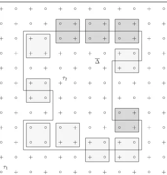
Fig. 1 A contour bordering the regionseparating blocksCτ1 andCτ2 with configurationsGeandGo, respectively. Spins with values+1,−1, are denoted by+,◦. The solid line represents the boundary of the region, with the minimal cutsetγconsisting of 20 edges corresponding to pairs of blocks touching the boundary from both sides—12 edges aligned in directione2(represented by horizontal pieces of the boundary)
and 8 edges aligned in directione1. The darker shaded blocks are those at least 1/2 of then/(2d)bad blocks
fromS(γ ), all belonging to the same partition: in our case the new partition ofTLwith the basic blockC
shifted by a unit vector fromTLin the directione2
To prove Lemma3.3we use Peierls’ argument hinging on chessboard estimates in a version inspired by the proof of Lemma 4.2 in [2].
3.3 Peierls’ Argument
For a given Ising configuration, consider the eventτ2τ1(Ge)∩τ2τ2(Go)that the blocksCτ1and Cτ2 have different staggered configurations described byGeandGo, respectively. The idea is to show the existence of a contour separating the pointsτ1andτ2and to use chessboard
[image:11.439.51.392.42.398.2]Consider the set of all blocks (labeled by)τ ∈TL/2 such that a translation of the even
staggered configurationτ2τ(Ge)occurs on it. Let ⊂ TL/2 be its connected component
containingτ1. Consider the component⊂TL/2ofccontainingτ2. The set of edgesγ
of the graphTL/2between vertices ofand its complementcis a minimal cutset of.
Informally,γ is a contour betweenwith all its holes except the one containingτ2filled up
and the remaining component containingτ2—a contour separatingτ1andτ2. The standard
fact is that the number of contours with a fixed number of edges|γ| = nseparating two verticesτ1andτ2is bounded bycnwith a suitable constantc.
Given a contourγ of length|γ| =n, there exists a coordinate direction such that there are at leastn/dedges inγaligned along this direction. Assuming, without loss of generality, that this is the “vertical” axised, precisely half of those edges have their outer endpoint (the
vertex in) “below” their inner endpoint. Thus, we can assume that there are at leastn/(2d) edges{τ, τ+ed}such thatτ ∈andτ+ed ∈.
Now, the crucial claim is that with each contour we can associate at least 1/2 of then/(2d) bad blocks (with a configuration fromϑ2τ(B)), all belonging to the same fixed partition: either
to our original partition ofTLlabelled byTL/2 or to a new partition ofTL with the basic
blockC shifted by a unit vector fromTLin directioned. Indeed, any block corresponding
to an outer vertexτ is either bad or, if not, it has to be a translation τ2τ(Go) of the odd
staggered configuration (being the even staggered configuration would be in contradiction with the assumption thatis a connected component of the set of blocks with even staggered configuration). However, then the block shifted by a unit vector inTLin directionedfeatures
an odd staggered configuration on its lower half and an even staggered configurations on its upper half, i.e., a configuration that belongs to the properly shifted setB(here it is helpful that the setBis invariant with respect to the reflection through the middle plane of the block). We useS(γ )to denote this collection of at least|γ|/(4d)bad blocks associated with contourγ. Given that, according to the construction above, all blocks fromS(γ )belong to the same partition (either the original one or a shifted one), we can use the chessboard estimate based on the the corresponding partition to bound the probability that all blocks of a given setS(γ )are bad by
τ∈S(γ )
ϑτ(B)
L, β ≤qL, β(B)
|S(γ )|. (3.35)
As a result, assuming thatqL, β(B) ≤1 (we will later show it can be made arbitrarily
small), the expectation of the eventτ2τ1(Ge)∩τ2τ2(Go)is bounded by
τ2τ1(Ge)∩τ2τ2(Go)
L, β
≤
γseparatingτ1andτ2
qL, β(B)|γ|/(4d)2|γ|/(2d)+1. (3.36)
Here, 2|γ|/(2d)+1is the bound on the number of setsS(γ )associated with the contourγ once the directioned is chosen.
This leads to the final bound
τ2τ1(Ge)∩τ2τ2(Go)
L, β
≤ ∞
n=4
24qL, β(B)n/(4d)
cn. (3.37)
We now see that Lemma3.3will hold ifqL, β(B)can be made arbitrarily small by tuning
the parameters of the model correctly. Hence we turn our attention to this.
Fig. 2 Example of a disseminated pattern obtained by reflections of a configuration fromB(3)onC(inside the shaded box). Notice that the configurations on blocks shifted byτwith both coordinates even are just translations of the original configuration onC
Ford =2, the setBconsists of 14 configurations that can be classified into five events according to the number of sites inC that have Ising spin+1,B = B(0)∪B(1)∪B(2)∪
B(3)∪B(4). Here, B(0) andB(4)consist of a single configuration (fully−1 and fully+1,
respectively) andB(1),B(2),B(3) consist each of 4 configurations related by symmetries. Notice that the eventB(2)has precisely two+1 spins at neighbouring positions (excluding the configurationsσeandσo). The case ofB(3)is depicted in Fig.2.
By subadditivity we can bound qL, β(B) by the sum of expectations of homogenised
patterns based on the fourteen configurations fromB disseminated throughout the lattice by reflections. In view of the symmetries, we need only consider only 5 configurations σ(k),k=0,1, . . . ,4, one from each eventB(k),k =0,1, . . . ,4. In fact we can see that, as
reflections flips the sign of Ising variables, that we need only considerk = 0,1,2 Indeed, the dissemination of patternB(0)differs from the dissemination of patternB(4)by a shift by 2e1, and the dissemination of patternB(1)differs from the dissemination of patternB(3)by
a shift by 2e1and a rotation.
We useZ(Lk)(β)to denote the corresponding quantities
Z(Lk)(β)=qL, β({σ(k)})(L/2)
2
ZL(β), (3.38)
fork∈ {0,1, . . . ,4}. For notational consistency we also denote the contribution of staggered configurations onTL asZ(Le)(β)andZ(
o)
[image:13.439.63.370.47.344.2]Lemma 3.4 For anyμ∈Randκ < κ0(μ)we have
Z(L0)(β),ZL(4)(β)≤eβL2|μ|STr exp ⎧ ⎨ ⎩ β S2
{x,y}
(S(x1)S(y1)+S(x3)S(y3)) ⎫ ⎬
⎭, (3.39)
Z(L1)(β),ZL(2)(β),Z(L3)(β)≤eβL
2 |μ|S−κ+S+1
S Tr exp ⎧ ⎨ ⎩ β S2
{x,y}
(Sx(1)S(y1)+Sx(3)S(y3)) ⎫ ⎬ ⎭,
(3.40)
Z(Le)(β),Z(Lo)(β)≥eβL
2 −|μ|S−2κ+2S+1
S Tr exp ⎧ ⎨ ⎩ β S2
{x,y}
(Sx(1)S(y1)+Sx(3)S(y3)) ⎫ ⎬ ⎭.
(3.41)
Proof We begin by removing the terms associated toS(S+1), κandμfrom the Hamilto-nian, i.e., we need bounds on the terms(−S+S1 +κ){x,y}σx(k)σy(k)andμ
x∈TLσ
(k)
x S(x3)
(occuring in−H), forσ(k), the Ising configuration corresponding to the disseminated pattern
B(k).
For the first term we use that σx(k)σy(k) = ±1 for each{x,y}. In particular, we get
{x,y}σ(
k)
x σy(k) = 0 for k = 0,4, it equals −L2 for k = 1,2,3, and it equals −2L2
fork=e,o. Indeed, forσ(0)andσ(4)half of the links yield−1 (they are are between aplus
and aminus) and the second half yield+1. Forσ(1),σ(2), andσ(3)three quarters of the links yield−1 and one quarters+1. Finally, fork=e andk=o all links yield−1.
For theμ-term we use the simple bound
− |μ|S L2≤μ "" "" ""x∈TL
σxS(x3)
"" ""
""≤ |μ|S L2. (3.42) Together this gives the factors in front of the traces in equations (3.39), (3.40), and (3.41). What remains in each case is a term of the form
− 1 S2
{x,y}
σ(k)
x σy(k)(Sx(1)Sy(1)+S(x3)S(y3)) (3.43)
wherek ∈ {0,1, . . . ,4,e,o}. By conjugating with a unitary operator acting aseiπS2on the
sites whereσx(k)= −1 we can turn this operator into,
− 1 S2
{x,y}
(Sx(1)S(y1)+Sx(3)S(y3)). (3.44)
As we have conjugated by a unitary operator this conjugation does not affect the trace. This
completes the proof.
As a result, we get the following bounds on the expectations of the disseminated bad configurationsqL, β({σ(k)})fork=0,1, . . . ,4.
Lemma 3.5 Letμ∈Randκ < κ0(μ). We have
qL,β({σ(0)}),qL,β({σ(4)})≤2−4/L
2
exp#4β2|μ|S+2κ−2S+S1$ (3.45)
Proof All the estimates follow from the previous lemmas using
qL, β({σ(k)})=
% Z(Lk)(β)
ZL(β)
&(2/L)2
≤ %
Z(Lk)(β) 2ZeL(β)
&(2/L)2
. (3.47)
Further, using subadditivity (Lemma3.2) we have
qL, β(B)≤qL, β({σ(0)})+4
3
k=1
qL, β({σ(k)})+qL, β({σ(4)}). (3.48)
From Lemma3.5we can see that forβlarge this quantity will be small if
κ <min{1+ 1S− |μ|S,1+ 1S −2|μ|S} =1+1S −2|μ|S=:κ0(μ). (3.49)
This condition is compatible with the requirementκ ≤1+ 1S in Lemma3.2and allows us to takeκ >0 once|μ|< 21S +21S2.
More precisely, we see that there existsμ0 > 0 and a functionκ0 that is positive on
(−μ0, μ0)such that if|μ|< μ0,κ <max(κ0(μ),0), andε >0, there existsβ0(μ, κ, ε)
such that the claims of Lemma3.3and thus also Theorem2.1are valid for anyβ≥β0.
Acknowledgements The research of R.K. was supported by the Grant GA ˇCR 16-15238S and that of B.L. partially by EPSRC grant EP/HO23364/1 and partially by the Alexander von Humboldt Foundation. R.K. would also like to thank the Isaac Newton Institute for Mathematical Sciences for support and hospitality during the programmeScaling limits, rough paths, quantum field theory(supported by EPSRC Grant No. EP/R014604/1) where the work on the final version of the paper was undertaken. We also thank the anonymous referee for suggesting to comment on differences with the Falicov–Kimball model and Daniel Ueltschi for useful explanations in this context.
Open Access This article is distributed under the terms of the Creative Commons Attribution 4.0 International License (http://creativecommons.org/licenses/by/4.0/), which permits unrestricted use, distribution, and repro-duction in any medium, provided you give appropriate credit to the original author(s) and the source, provide a link to the Creative Commons license, and indicate if changes were made.
References
1. Biskup, M.: Reflection positivity and phase transitions in lattice spin models. Methods of Contemporary Mathematical Statistical Physics. Lecture Notes in Mathematics, vol. 1970, pp. 1–86. Springer, Berlin (2009)
2. Biskup, M., Chayes, L., Starr, S.: Quantum spin systems at positive temperature. Commun. Math. Phys. 269, 611–657 (2007)
3. Chayes, L., Kotecký, R., Shlosman, S.: Aggregation and intermediate phases in dilute spin systems. Commun. Math. Phys.171, 203–232 (1995)
4. Chayes, L., Kotecký, R., Shlosman, S.: Staggered phases in diluted systems with continuous spins. Commun. Math. Phys.189, 631–640 (1997)
5. Dyson, F.J., Lieb, E.H., Simon, B.: Phase transitions in quantum spin systems with isotropic and non-isotropic interactions. J. Stat. Phys.18, 335–383 (1978)
6. Fröhlich, J., Israel, R., Lieb, E., Simon, B.: Phase transitions and reflection positivity. I. General theory and long range lattice models. Commun. Math. Phys.62, 1–34 (1978)
7. Fröhlich, J., Israel, R., Lieb, E., Simon, B.: Phase transitions and reflection positivity. II. Lattice systems with short-range and Coulomb interactions. J. Stat. Phys.22, 297–347 (1980)
9. Fröhlich, J., Simon, B., Spencer, T.: Infrared bounds, phase transitions and continuous symmetry breaking. Commun. Math. Phys.50, 79–95 (1976)
10. Gruber, C., Macris, N.: The Falicov–Kimball model: a review of exact results and extensions Hel. Phys. Acta.69, 850–907 (1996)
11. Gruber, C., Macris, N., Messager, A., Ueltschi, D.: Ground states and flux configurations of the two-dimensional Falicov–Kimball model. J. Stat. Phys.86, 57–108 (1997)
12. Lebowitz, J.L., Macris, N.: Long range order in the Falicov-Kimball model: extension of Kennedy–Lieb Theorem Rev. Math. Phys.6, 927–946 (1994)
13. Robinson, D.: Statistical mechanics of quantum spin systems. II. Commun. Math. Phys.7, 337–348 (1968)