Optimal Input Excitation Design for Nonparametric Uncertainty Quantification of Multi Input Multi Output Systems

of Multi-Input Multi-Output Systems

Atta Oveisi*, Ashlee Anderson*, Tamara Nestorović*, Allahyar Montazeri**

* Ruhr-Universität Bochum, Mechanics of Adaptive Systems (MAS), Bochum D-44801, Germany ([email protected]).

** Engineering Department, Lancaster University, Lancaster LA1 4YW, UK ([email protected]).

Abstract: In this paper, the impact of various input excitation scenarios on two different MIMO linear non-parametric modeling schemes is investigated in the frequency-domain. It is intended to provide insight into the optimal experiment design that not only provides the best linear approximation (BLA) of the frequency response functions (FRFs), but also delivers the means for assessing the variance of the estimations. Finding the mathematical representations of the variances in terms of the estimation coherence and noise/nonlinearity contributions are of critical importance for the frequency-domain system identification where the objective function needs to be weighted in the parametrization step. The

input excitation signal design is tackled in two cases, i.e., multiple single-reference experiments based on

the zero-mean Gaussian and the colored noise signal, the random-phase multisine, the Schroeder

multisine, and minimized crest factor multisine; and multi-reference experiments based on the Hadamard

matrix, and the so-called orthogonal multisine approach, which additionally examines the coupling

between the input channels. The time-domain data from both cases are taken into the classical H1 spectral

analysis as well as the robust local polynomial method (LPM) to extract the BLAs. The results are applied for data-driven modeling of a flexible beam as a model of a flexible robotic arm.

Keywords: Modal Analysis; Optimal experiment; Multisine excitation; Uncertainty Modeling.

 1. INTRODUCTION

Contemporary applications of robot arms demand high precision and speed, e.g. advanced manufacturing and nuclear decommissioning. These applications typically require accurate knowledge of the dynamic model of robot arm (Montazeri and Ekotuyo, 2016). Experimental identification and parameter calibration are therefore the only reliable approach to obtain this information (Montazeri et al, 2017). Input excitation design plays an important aspect of this procedure by optimizing a few variables such as operational bandwidth of the system, maximum permissible excitation amplitude on the actuators, and the sampling time limitations before the task-overrun error. Among different excitation inputs multisine signal is proven to have minimum time-factor, i.e., minimum time per frequency for reaching a specified signal-to-noise ratio (SNR). It is also effective in terms of measurement duration, accuracy, and sensitivity to noise/nonlinearity compared to other signal types (Schoukens et al. 1988). Since this work, several attempts have been made to improve the energy content of the signal, i.e., the property of having a low crest factor (CF) for the input/output data. Consequently, CF minimization is shown to secure a desirable quality in signal processing namely, a high SNR (Guillaume et al. 1991).

Here we take the first step on data-driven modelling of a MIMO robotic system by assuming a flexible arm as a lightly damped flexible beam. Frequency response functions (FRFs) are proven to confer in-depth insight into the behaviour of the complex dynamical systems. Modal tests using the spectral

analysis technique is well-studied for parametric estimation of the single-input single output dynamic systems (Montazeri et al. 2009; Montazeri et al. 2011; Ahmadizadeh et al. 2015). However, the estimation procedure of the FR matrix (FRM) for the multivariable systems is technically much more involved as it uses the cross-correlation techniques which yield the input excitations to be uncorrelated. Apart from the low-frequency resolution method proposed in (Zhang et al. 2010) and not intended for lightly damped smart structures, one of the major issues of random excitations is that no differentiation between noise and nonlinearity can be deduced from the results.

Contrary to H1/H2 functions in the spectral analysis, FRM

and its covariance matrices can be calculated following (Pintelon, Barbé, et al. 2011). Several consecutive periods and several independent realizations of the multi-reference tests should be performed, which in turn provides the means for acquiring the sample means and sample (co-)variances of the input/output spectra. The latter is realized while attenuating the stochastic noise and transients.

robust local polynomial method (LPM) in nonparametric modelling. To this end, several advantages of extracting the statistical properties of the obtained FRM, e.g. estimation variance in regards to the noise/nonlinearity, in the latter method are highlighted, which are crucial for the parametric system identification, the state estimation problem, and the robust control design. The procedure as shown in this paper amounts to a substantial reduction in the experimental time which may be very expensive in the scope of the light weight aerospace systems. The plant is shown in Fig. 1, while geometric dimensions, the material properties of the four piezo-actuator patches and the aluminium host, the technical details of the measurement setup, and sensor and actuator placement optimization are all referred to (Oveisi & Nestorović 2016b). The system has five inputs, including four collocated actuators (two on each side of the beam) and a shaker, as well as two outputs viz. a laser Doppler vibrometer (LDV) collocated with a 1D accelerometer at the free end of the beam. In the rest of the paper, indicates the

unit imaginary number, is the frequency of the line in

the continuous spectrum of the signal, and the hat operator

.̂ and zero subscript ( ) symbolize the estimated and

unknown correct values of the associated variables, respectively. Capital letters are used for the frequency-domain data obtained using FFT while lower case variables are reserved for the sampled time-domain signals.

Fig. 1. The experimental rig for the system identification.

2. EXPERIMENT DESIGN

It is expected that measurement data is affected by erroneous stochastic noise, the extent of which depends on the measurement methods and the instruments involved. Additionally, morphing dynamic systems often have long-lasting transient behaviour under periodic loading, which contributes as an additional source of imperfection in the results of the post-processing phase. Unlike the stochastic noise and transients in the response, the effect of nonlinearities in the system output persists even after long measurements for suppressing the non-steady state history and after averaging over multiple periods.

2.1 Single-reference Experiments

In the single-reference (SR) modal analysis scheme, the input excitation design is initiated with a random Gaussian zero-mean signal (RGS). In order to be able to capture the higher

order nonlinearities, the sampling time is set to 122.07 µs ( 10 times higher than the maximum operational frequency) following the literature in the nonlinear system identification.

Additionally, 2 lines are considered in the Fourier analysis

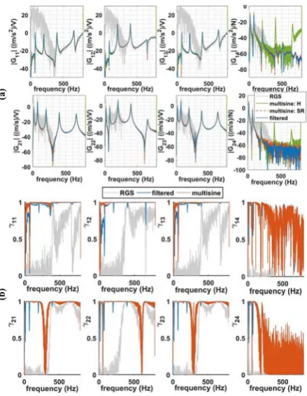
to guarantee sufficient number of samples in the 3dB range of the resonance frequencies in the framework of LPM (Pintelon, Vandersteen, et al. 2011). As one would expect, the coupling between the input channels is neglected in the single-reference experiments. The FRFs of the system based on the RGS excitations is then compared with the coloured noise excitation and the random-phase multisine. To this end, individual experiments are performed for ten periods of each excitation signal to quantify the contribution of the transient noise. The distorted periods in the input/output data are then discarded, followed by a spectral analysis of the remaining time history. In Fig. 2(a), the frequency content of the two random signals are compared to the periodic random-phase multisine excitation. Unlike the RGS, the multisine excitation has a slight advantage in terms of band-limited analysis since it has insignificant contribution over other frequencies. Though the coloured noise signal also satisfies the band-limited constraint of the desired excitation, it is categorized as a non-periodic signal and is thus subjected to leakage errors. The contribution of the transients under multisine periodic excitation for the two measurement outputs is evaluated in Fig. 2(b). It can be seen that the transient response falls below the noise floor within two consecutive periods. Consequently, the response of the first period is discarded in the classical spectral analysis based on the function.

Fig. 2. (a) Frequency content of the input excitation signals. (b) Contribution of transient noise over two periods.

For a periodic multisine signal with a high SNR, it can be shown that under reasonable experimental conditions, e.g.,

averaging over the periods, we have .

However, for random excitations, even neglecting the effect of persistent structural nonlinearities, a biased estimation of

the FRFs, given by 1 ⁄

⁄ , is still expected since the measurement

output and excitation input are polluted by stochastic

noise , and , respectively. The systematic error in

random excitation cannot be resolved unless the SNR for the

input signal generator (| | ≫ | |) is high. Under the

assumption that the SNR at the input is higher than that of the

output, (as opposed to ) estimation is used to calculate

the FRFs as / . The FRFs of the system

of the paper, each subplot indicates the FRF from the piezo-actuators and shaker to the measurement outputs, (accelerometer and LDV), represented in columns 1-4 or 1-5, and rows 1-2, respectively. As a measure of the FRF quality, the coherence of the captured output w.r.t. the input as a measure of the FRF quality is shown in Fig. 3(b). In Figs. 3(a) and (b), the first period of the periodic excitation is discarded to suppress transient distortions, and a Hann-window with 80 averages is used to reduce the leakage errors for the two non-periodic inputs.

The observations are as follows: 1) The RGS signal has the worst coherence, and as a result, the obtained FRFs are unreliable. As pointed out in (Pintelon et al. 2012), although the clipped random noise with uniform distribution has a better performance than the RGS, it is recommended to pre-filter (blue lines in Fig. 3) the excitation signal with/without sign operation (random binary excitation). 2) Despite the similarity between the FRFs of the MIMO system in Fig. 3(a) for both filtered noise and multisine (multisine: SR) signals, the coherence comparison in Fig. 3(b) reveals the superiority of the estimation quality of the multisine signal. 3) The coherence of all signals in the vicinity of the anti-resonance frequencies drops significantly below 1. In the case of multisine, this can be remedied by replacing the uniform distribution of the excitation lines with a spectrum configuration with populated lines around anti-resonances. This guarantees the injection of enough energy at those frequency ranges, resulting in a higher SNR. However, there is a trade-off between reduced resampling time of the

(a)

(b)

Fig. 3. (a) Magnitude of FRFs in dB range based on three single-reference loading and Hadamard multi-reference scenarios. (b) Coherence diagram of the measured FRFs.

experiment, which may result in hardware memory shortage that is of particular concern in practical situations involving lightly-damped structures with long transient behaviour and consequently lengthy measurements. 4) In order to investigate the input coupling, or in other words, the essence of performing multi-reference modal analysis instead of multiple single-reference ones, the BLA based on the Hadamard multisine method is compared with single-reference results. Fig. 3(a) indicates that the multi-single-reference excitation (the green line, multisine: H) and the calculated FRFs, excluding the shaker channel, have similar outcomes. Although no apparent coupling between the piezo-patches is observed, the distorted FRF associated with the shaker (and both outputs) is evidence of input coupling between the shaker and the piezo-patches. This behaviour is due to the flexible assembly of the shaker and the beam which are connected to each other via rubber-band as shown in Fig. 1. It should be noted that the aforementioned coupling is no longer observed when the shaker and beam are connected via a screw (Oveisi & Nestorović 2016a). It is important to note that the crest factor of the excitation signals is not changed in the multi-reference scenario unless, as is the case for the shaker input coupling, similar non-parametric modelling results are expected.

2.2 Multi-reference Experiments

In the multi-reference analyses (for number of input channels), two scenarios are investigated based on the number of input signals: 1) The case where three piezo-actuators (realizing the control inputs) along with the shaker (realizing the mismatch disturbance channel), are included in the Hadamard multisine approach, i.e., four channels to

satisfy the radix-2 condition, i.e., 2 (Pintelon et al.

2012). In this approach, the single-reference signal is

multiplied by the Hadamard matrix 1/ where

⨂ , 1,1; 1, 1 , (in MATLAB matrix

notation). The Kronecker matrix product is represented with

⨂. Experimentally, Hadamard multisine is realized by

employing a set of inverters. 2) The case of an orthogonal multisine based on the multi-generator approach for an odd number of inputs (four piezo-actuators and the shaker) is carried out according to (Dobrowiecki et al. 2006). Unlike the Hadamard multisine where the number of input channels must satisfy radix-2 condition, the so-called orthogonal multisine can be used for an arbitrary number of input channels with the orthogonal elements of the matrix given by

, / exp 1 1 / for , 1, … , .

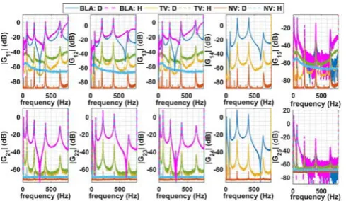
Fig. 4. BLA of the FRF using Hadamard matrix approach (H) and orthogonal multisine (D) as well as noise variance (NV) and total variance (TV).

experiments require independent generators. The standard deviation of the excitation signals in both cases is retained at 0.75 to keep the actual implemented signals on the piezo-actuators beneath 250 V in amplitude. Fig. 4 presents the results of the robust LPM based on the two multi-reference schemes.

The following observations can be made based on the results shown in Fig. 4: 1) As expected unlike the accelerometer, the contactless LDV is less prone to noise. This can be deduced from the matching quality between the two multi-reference schemes as well as from the significant difference between the acceleration measurements. 2) For the same RMS value of the excitation signal, BLAs obtained from the Hadamard single-generator matrix method have higher total variance in comparison to the orthogonal multisine scheme. This is justifiable by examining the noise floor in the two cases, i.e., comparing NV:D and NV:H for the accelerometer, which indicate high achievable SNR in the orthogonal multisine approach.

Consequently, the orthogonal approach is preferred for parameterized modeling. 3) The FRFs associated with the shaker input are severely distorted at frequencies higher than 100 Hz. Unlike the classical function in Fig. 3(a) and its coherence in Fig. 3(b) which indicate unreliable modelling quality at these frequencies, the source of distortions in the robust MIMO LPM method of (Pintelon, Vandersteen, et al. 2011) are associated with noise/nonlinear contributions. Physically, the nonlinear distortion is due to the nature of the connection between the shaker and the beam, i.e., the rubber-band (see Fig. 1). The reason for using a rubber-rubber-band instead of a direct connection (adhesive wax, screws, etc.) is to match the impedance of the (control) input signals realized by the piezo-patches with the (disturbance) signal generated by the electromagnetic shaker (Pintelon et al. 2012). 4) In the results of the orthogonal multisine method, the contribution of nonlinear distortions can be neglected since the total variance is 40 dB below the BLA. However, depending on the application, this may become non-negligible. Before proceeding to the assessment of input excitation optimization in MIMO smart structures, two remarks should be made regarding the importance of the MIMO robust LPM: a) The total variance not only reflects the quality of the estimated

FRFs, but also provides a tool for quantifying the modelling uncertainty which is crucial in robust control design. Additionally, it provides the means for state observer design techniques, e.g., Kalman filter that may be used in output feedback control by quantifying the process/measurement noise’s covariance matrices. b) The parameterization of the calculated BLAs based on the black/grey-box subspace method reduces to a weighted regression problem where the obtained total variance from the MIMO LPM serves as the frequency-dependent weighing without which the estimated linear model would be biased (McKelvey et al. 1996; Cavallo et al. 2007).

3. INPUT EXCITATION OPTIMIZATION

3.1. Crest Factor Minimization

Since the spectrum of the employed signal is known a priory,

the minimization of the CF is defined in terms of the random phases associated with the active line in the multisine excitation. Since the CF-minimized multisine is unique, the contribution of the nonlinearity (using several random realizations) is not quantifiable in the framework of the robust LPM. On the other hand, as an advantage of CF minimization, the number of required averages for a specific accuracy regarding the SNR at low-frequency ranges, where the experiment durations are lengthy, is proportional to the square of the CF.

Mathematically, the CF of a time-dependent vector is

defined as ‖ ‖ /‖ ‖ which is the

peak-value over the signal root mean square. Our analysis here is only concerned with optimizing the phases (excluding the zero line) of each line for a given auto-power spectrum. Since

the objective function ( ) is nondifferentiable, an

analytical optimization solution is unavailable. As a results, the Quasi-Newton (QN) algorithm, in which the Hessian matrix is estimated (updated) from the gradient vector, is implemented. Accordingly, the Hessian matrix is calculated by the Davidon-Fletcher-Powell (DFP) formula to mimic the Newton algorithm in computing the search direction (Griva et al. 2009). The algorithm is initialized by the Schroeder multisine, i.e., for line number and number of nonzero lines in the spectrum, the associated phase is initialized with

1 / . The optimization is carried out on a parallel

typically between 1.65-1.7 (Pintelon et al. 2012). Additionally, the CF associated with the random-phase

multisine for 10 realizations varied between 2.5 and 6.3,

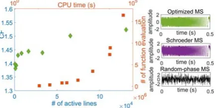
further emphasizing the importance of testing various random-phase multisine signals before deciding to use one in an experiment. Moreover, three subplots are added to Fig. 5 to compare the time history of the random-phase multisine, the Schroeder multisine, and the CF-optimized multisine for 2048 number of lines in the frequency range of interest. Although the random-phase multisine is similar to the stochastic noise, its amplitude spectrum is deterministic. Comparing the time histories of the Schroeder and minimized-CF multisine signals indicates the reduction in magnitude (despite higher injected energy per line) of for the optimized signals. Note that the optimization is done over each line in the frequency-domain as time-domain optimization causes more computational burden.

Fig. 5. Effect of the frequency resolution of the multisine excitation on the CF and subsequent computational overhead.

3.2. Multi-Reference Non-parametric Modelling with CF-minimized Multisine Excitation

The multi-reference (CF-minimized) signal, is applied to the system in Fig. 1 through the input channels. Then, the obtained time-histories are analysed with the robust LPM. Then the modal analyses of the optimized signal with 65536 line number and Nyquist frequency band of 2048 Hz is done for eight consecutive periods of the Hadamard and orthogonal multisine. Illustration of the results in Fig. 6, shows that the frequencies of the resonance states are the same for both the CF-optimized and the random-phase multisine cases in the multi-reference experiments (Fig. 4). However, the FRFs in the anti-resonances and transition frequencies between the resonances are significantly different. Noting that the noise floor is independent of the optimization (compare Figs. 6 and 4 for NV), it is essential to assess the introduced mismatch due to the CF minimization. To this end, a perturbation analysis of the clamped-free beam geometry in Fig. 1 is carried out in the operational frequency range using ABAQUS finite element (FE) software. It is observed that imperfect boundary conditions and the attached sensor configurations lead to the excitation of the torsional and in-plane mode shapes. Due to the higher energy content injected through the active lines of the multisine signal, the first and second in-plane and torsional modes are significantly excited. This distorts the FRFs associated with transverse vibrations. Hence, the frequencies the second in- plane mode that is irrelevant to the transverse vibration. The

Fig. 6. BLA based on optimized CF (CFO) using Hadamard multisine (H) and orthogonal multisine (D), the noise variance (NV) compared to random-phase multisine (black line).

transverse vibration modes associated with the frequencies 1, 2, 4, 6, and 9 in the BLAs of Fig. 6 are also plotted on top of the figure. Unless the user tends to identify these modes (torsional/in-plane) and the actuators can control them, the optimization approach may cause an incorrect interpretation of the system. Additionally, this method provides no insight from the BLA regarding nonlinear variance.

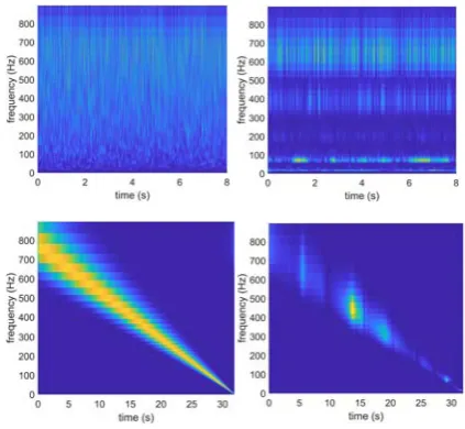
It should be noted that if the geometrical nonlinearities due to the large vibration amplitudes are relevant to the vibrations, CF minimization is not recommended since the total variance of the estimated BLAs is expected to increase significantly. This prediction is a direct result of invoking the higher-order strain terms in system dynamics (Oveisi & Nestorović 2017). This can be justified by 5nalysing the time-frequency content of the two cases i.e., random-phase multisine and CF-minimized multisine. To this end, the time-frequency analysis based on the continuous Morlet wavelet transformation (Noël & Kerschen 2017) is performed on the input/output data in the two cases, and the normalized results are shown in Fig. 7. In this figure, the top row is reserved for random-phase multisine while the bottom row is dedicated to the minimized CF. The first and second columns represent input and output, correspondingly. Unlike the random-phase multisine, the spectrum of the input in the case of minimized CF follows a specific line of harmonics which resembles the sweep-sine excitation. Consequently, the time-frequency analysis over the measurement output of the minimized CF case reveals that the energy of the input signal is injected at a specific frequency range at each time increment. However, the output of the system under random-phase multisine input indicates the random distribution of energy at all frequencies at each time sample. Despite the inability of the method to detect nonlinearities, CF minimization should be applied with care and is not recommended without proper insight on the system, especially in combination with black-box identification.

6. CONCLUSIONS

Several input excitation signals are tested experimentally and

in single-/multi-reference schemes are used to extract the FRM of the system. Moreover, quantified measures of the imperfections due to stochastic noise, transient distortion, and nonlinear structural behaviour are calculated. In addition to the technical conclusions in each case, several guidelines are provided for the Vibration Engineer regarding the selection of the optimal experiment configurations depending on the accuracy of involved measurement devices and the potential insight that one may have regarding the nonlinearity/noise level. The results of the paper enable not only the use of the estimated covariance matrices in both single-step, e.g., subspace method and iterative, e.g., predictive error method of parametric identification methods, but also facilitate lumped uncertainty quantification and state observer design.

Fig. 7. Time-frequency analysis of the input/output data

ACKNOWLEDGEMENTS

The work is supported by the Engineering and Physical Sciences Research Council (EPSRC), grant number EP/R02572X/1, and National Centre for Nuclear Robotics. The authors are grateful for the support of the National Nuclear Laboratory and the Nuclear Decommissioning Authority (NDA).

REFERENCES

Ahmadizadeh, S., Montazeri, A. & Poshtan, J., 2015. Design of minimax-linear quadratic Gaussian controller using the frequency domain subspace identified model of

flexible plate. Journal of Vibration and Control, 21(6),

pp.1115–1143.

Cavallo, A. et al., 2007. Gray-Box Identification of

Continuous-Time Models of Flexible Structures. IEEE

Transactions on Control Systems Technology, 15(5), pp.967–981.

Dobrowiecki, T.P., Schoukens, J. & Guillaume, P., 2006. Optimized excitation signals for MIMO frequency

response function measurements. IEEE Transactions

on Instrumentation and Measurement, 55(6), pp.2072– 2079.

Montazeri, A., West, C., Monk, S.D., Taylor, J., 2017. Dynamic modelling and parameter estimation of a

hydraulic robot manipulator using a multi-objective

genetic algorithm. International Journal of Control,

90(4), pp.661-683.

Montazeri, A., Ekotuyo, J., 2016. Development of dynamic model of a 7DOF hydraulically actuated tele-operated

robot for decommissioning applications. IEEE

American Control Conference (ACC), pp. 1209-1214

Griva, I., Nash, S. & Sofer, A., 2009. Linear and nonlinear

optimization, Society for Industrial and Applied Mathematics.

Guillaume, P. et al., 1991. Crest-factor minimization using

nonlinear Chebyshev approximation methods. IEEE

Transactions on Instrumentation and Measurement, 40(6), pp.982–989.

McKelvey, T., Akcay, H. & Ljung, L., 1996. Subspace-based multivariable system identification from frequency

response data. IEEE Transactions on Automatic

Control, 41(7), pp.960–979..

Montazeri, A., Poshtan, J. & Choobdar, A., 2009.

Performance and robust stability trade-off in minimax LQG control of vibrations in flexible structures.

Engineering Structures, 31(10), pp.2407–2413. Montazeri, A., Poshtan, J. & Yousefi-Koma, A., 2011.

Design and analysis of robust minimax LQG controller for an experimental beam considering spill-over effect.

IEEE Transactions on control systems technology, 19 (5), 1251-1259.

Noël, J.P. & Kerschen, G., 2017. Nonlinear system

identification in structural dynamics: 10 more years of

progress. Mechanical Systems and Signal Processing,

83, pp.2–35.

Oveisi, A. & Nestorović, T., 2016a. Mu-Synthesis based

active robust vibration control of an MRI inlet. FACTA

UNIVERSITATIS Series: Mechanical Engineering, 14(1), pp.37–53.

Oveisi, A. & Nestorović, T., 2016b. Robust observer-based

adaptive fuzzy sliding mode controller. Mechanical

Systems and Signal Processing, 76–77, pp.58–71. Oveisi, A. & Nestorović, T., 2017. Transient response of an

active nonlinear sandwich piezolaminated plate.

Communications in Nonlinear Science and Numerical Simulation, 45, pp.158–175.

Pintelon, R., Barbé, K., et al., 2011. Improved (non-)parametric identification of dynamic systems excited

by periodic signals. Mechanical Systems and Signal

Processing, 25(7), pp.2683–2704.

Pintelon, R., Vandersteen, G., et al., 2011. Improved (non-) parametric identification of dynamic systems excited

by periodic signals—The multivariate case. Mechanical

Systems and Signal Processing, 25(8), pp.2892–2922.

Pintelon, R. , Schoukens, J., 2012. System identification : a

frequency domain approach, Wiley.

Schoukens, J. et al., 1988. Survey of Excitation Signals for

FFT Based Signal Analyzers. IEEE Transactions on

Instrumentation and Measurement, 37(3), pp.342–352. Zhang, E. et al., 2010. Fast detection of system nonlinearity

using nonstationary signals. Mechanical Systems and