Two Roads to Planet Detection

(1)

Two roads to planet detection

Thesis by

Michael Bottom

In Partial Fulfillment of the Requirements

for the Degree of

Doctor of Philosophy

California Institute of Technology

Pasadena, California

2016

(2)

c

2016 Michael Bottom

(3)

To my parents,

(4)

(5)

Acknowledgments

It was, gentlemen, after a long absence—seven years to be exact, during which time I was studying in Europe—that I returned to my people. I learnt much and much passed me by—but that’s another story. The important thing is that I returned with a great yearning for my people in that small village at the bend of the Nile. For seven years I had longed for them, had dreamed of them, and it was an extraordinary moment when I at last found myself standing amongst them. They rejoiced at having me back and made a great fuss, and it was not long before I felt as though a piece of ice were melting inside of me, as though I were some frozen substance on which the sun had shone—that life warmth of the tribe which I had lost for a time in a land “whose fishes die of the cold.” My ears had become used to their voices, my eyes grown accustomed to their forms. Because of having thought so much about them during my absence, something rather like fog rose up between them and me the first instant I saw them. But the fog cleared and I awoke on the second day of my arrival, in my familiar bed in the room whose walls had witnessed the trivial incidents of my life in childhood and the onset of adolescence. I listened intently to the wind: that indeed was a sound well known to me, a sound which in our village possessed a merry whispering—the sound of the wind passing through palm trees is different from when it passes through fields of corn. I heard the cooing of the turtle-dove, and I looked through the window at the palm tree standing in the courtyard of our house and I knew that all was still well with life. I looked at its strong straight trunk, at its roots that strike down into the ground, at the green branches hanging down loosely over its top, and I experienced a feeling of assurance. I felt not like a storm-swept feather but like that palm tree, a being with a background, with roots, with a purpose.

-Tayeb Salih,Season of Migration to the North

It is proper and right to begin by thanking Professors Shri Kulkarni and John Johnson, my

advisors, who mostly left me alone to make my own progress and learn from my own mistakes, as

I preferred. I respect that. Similarly, I must thank Dr. Eugene Serabyn, my supervisor at the Jet

Propulsion Lab, for his insight and leadership. I owe special thanks to Professor Dimitri Mawet,

who was a patient teacher, collaborator, and mentor through my last years as a graduate student.

His ideas are all over this thesis, and it’s so much the better for that.

I’d like to thank the folks at NASA, whose names I don’t even know, who saw fit to support me

with the Space Technology Research Fellowship. It has made an enormously positive impact in the

course of my research.

I owe very much to postdocs Phil Muirhead and Jon Swift. Phil taught me an enormous amount,

and was a mentor and friend to me. Jon Swift was a great project manager and is a true Renaissance

(6)

who let me get knee deep in a fun second-year project, which gave me many skills I continue to draw

on to this day.

I must thank Chris Shelton and Kent Wallace, brilliant engineers from JPL, the best in the

business, who taught me so much about optics and instrumentation. I hope to be more like them

some day.

I thank the exceptional staff at Palomar Observatory, especially Steve Kunsman–may he have a

long and happy retirement. I will remember the many pleasant days and evenings at the magnificent

Hale telescope for the rest of my life.

I’d like to thank all my teachers here at Caltech, both the good and the bad. Teachers don’t get

enough credit: when I came in here, I barely knew what a “magnitude” was; now, I can impress the

hell out of anyone sitting next to me on an airplane, especially in economy class.

I owe much to my friends who made this journey so enjoyable: Brandon Dotson, the first person

I met at Caltech and the most badass; Brett and Huilin Cornell, constant companions, pundits, and

the first (and as of yet, only) two members of my ministerial flock; Abhilash Mishra and Io Kleiser,

brilliant and fierce members of la R´esistance; Leon Harding, a great Irish import and high flyer; Sirio Belli, for (or despite?) sharing an office for the better part of five years.

One more friend: Professor Wallace Sargent. Wal was an extraordinary person, with a great

sense of humor, warm personality, and sharp mind. I loved chatting in his office about everything

under the sun, and occasionally things beyond it. His passing left a huge hole in the department

that can never be filled. I miss him.

I owe the most to Heather Duckworth, who has been my partner and best friend during this

whole circus, and who I hope to partially repay in the coming decades. Here’s to getting on with

(7)

Abstract

One of the most exciting discoveries in astrophysics of the last last decade is of the sheer diversity

of planetary systems. These include “hot Jupiters”, giant planets so close to their host stars that

they orbit once every few days; “Super-Earths”, planets with sizes intermediate to those of Earth

and Neptune, of which no analogs exist in our own solar system; multi-planet systems with planets

smaller than Mars to larger than Jupiter; planets orbiting binary stars; free-floating planets flying

through the emptiness of space without any star; even planets orbiting pulsars. Despite these

remarkable discoveries, the field is still young, and there are many areas about which precious little

is known. In particular, we don’t know the planets orbiting Sun-like stars nearest to our own solar

system, and we know very little about the compositions of extrasolar planets. This thesis provides

developments in those directions, through two instrumentation projects.

The first chapter of this thesis concerns detecting planets in the Solar neighborhood using

preci-sion stellar radial velocities, also known as the Doppler technique. We present an analysis

determin-ing the most efficient way to detect planets considerdetermin-ing factors such as spectral type, wavelengths

of observation, spectrograph resolution, observing time, and instrumental sensitivity. We show that

G and K dwarfs observed at 400-600 nm are the best targets for surveys complete down to a given

planet mass and out to a specified orbital period. Overall we find that M dwarfs observed at 700-800

nm are the best targets for habitable-zone planets, particularly when including the effects of

system-atic noise floors caused by instrumental imperfections. Somewhat surprisingly, we demonstrate that

a modestly sized observatory, with a dedicated observing program, is up to the task of discovering

such planets.

We present just such an observatory in the second chapter, called the “MINiature Exoplanet

Radial Velocity Array,” or MINERVA. We describe the design, which uses a novel multi-aperture

approach to increase stability and performance through lower system etendue, as well as keeping

costs and time to deployment down. We present calculations of the expected planet yield, and

data showing the system performance from our testing and development of the system at Caltech’s

campus. We also present the motivation, design, and performance of a fiber coupling system for

the array, critical for efficiently and reliably bringing light from the telescopes to the spectrograph.

(8)

in Arizona.

The second part of this thesis concerns a very different method of planet detection, direct

imag-ing, which involves discovery and characterization of planets by collecting and analyzing their light.

Directly analyzing planetary light is the most promising way to study their atmospheres,

forma-tion histories, and composiforma-tions. Direct imaging is extremely challenging, as it requires a high

performance adaptive optics system to unblur the point-spread function of the parent star through

the atmosphere, a coronagraph to suppress stellar diffraction, and image post-processing to remove

non-common path “speckle” aberrations that can overwhelm any planetary companions.

To this end, we present the “Stellar Double Coronagraph,” or SDC, a flexible coronagraphic

platform for use with the 200” Hale telescope. It has two focal and pupil planes, allowing for a

number of different observing modes, including multiple vortex phase masks in series for improved

contrast and inner working angle behind the obscured aperture of the telescope. We present the

motivation, design, performance, and data reduction pipeline of the instrument. In the following

chapter, we present some early science results, including the first image of a companion to the star

delta Andromeda, which had been previously hypothesized but never seen.

A further chapter presents a wavefront control code developed for the instrument, using the

technique of “speckle nulling,” which can remove optical aberrations from the system using the

deformable mirror of the adaptive optics system. This code allows for improved contrast and inner

working angles, and was written in a modular style so as to be portable to other high contrast imaging

platforms. We present its performance on optical, near-infrared, and thermal infrared instruments

on the Palomar and Keck telescopes, showing how it can improve contrasts by a factor of a few in

less than ten iterations.

One of the large challenges in direct imaging is sensing and correcting the electric field in the

focal plane to remove scattered light that can be much brighter than any planets. In the last

chapter, we present a new method of focal-plane wavefront sensing, combining a coronagraph with

a simple phase-shifting interferometer. We present its design and implementation on the Stellar

Double Coronagraph, demonstrating its ability to create regions of high contrast by measuring and

correcting for optical aberrations in the focal plane. Finally, we derive how it is possible to use

the same hardware to distinguish companions from speckle errors using the principles of optical

coherence. We present results observing the brown dwarf HD 49197b, demonstrating the ability to

detect it despite it being buried in the speckle noise floor. We believe this is the first detection of a

(9)

Published content and

contributions

(See Section 1.5.2 for more details)

1. Bottom, Michael, Philip S. Muirhead, John Asher Johnson, and Cullen H. Blake. “Optimizing

Doppler Surveys for Planet Yield.” Publications of the Astronomical Society of the Pacific

125, no. 925 (2013): 240-251.

M.B. wrote and performed the numerical simulations, derived the different figures of merit,

produced all the figures, and prepared the manuscript.

2. Swift, Jonathan J., Michael Bottom, John A. Johnson, Jason T. Wright, Nate McCrady,

Robert A. Wittenmyer, Peter Plavchan et al. “Miniature Exoplanet Radial Velocity Array

(MINERVA) I. Design, Commissioning, and First Science Results.” Journal of Astronomical

Telescopes, Instruments, and Systems, Volume 1, Issue 2 (21 April 2015)

M.B. selected and tested much of the hardware, built and tested the pointing control

sys-tem, wrote the telescope controls software, performed many of the commissioning tests and

observations, and contributed to the manuscript preparation

3. Bottom, Michael, Philip S. Muirhead, Jonathan J. Swift, Ming Zhao, Paul Gardner, Peter P.

Plavchan, Reed L. Riddle et al. “Design, motivation, and on-sky tests of an efficient fiber

cou-pling unit for 1-meter class telescopes.” In SPIE Astronomical Telescopes+ Instrumentation,

pp. 91472E-91472E. International Society for Optics and Photonics, 2014.

M.B. contributed to the design of the unit, constructed it, wrote the control software and

simulations, and designed and performed the verification tests.

4. Bottom, M., J. C. Shelton, J. K. Wallace, R. Bartos, J. Kuhn, D. Mawet, B. Mennesson, R.

Burruss, E. Serabyn. “Stellar Double Coronagraph: a multistage coronagraphic platform at

Palomar observatory” Publications of the Astronomical Society of the Pacific, in press

M.B. contributed to the construction of the instrument and initial alignment and

commission-ing, wrote the pointing control/adaptive optics system software, performed the observations,

(10)

5. Bottom, Michael, Jonas Kuhn, Bertrand Mennesson, Dimitri Mawet, Jean C. Shelton, J. Kent

Wallace, Eugene Serabyn. “Resolving the delta Andromedae spectroscopic binary with direct

imaging”. The Astrophysical Journal, 809, 11 (June 2015)

M.B. performed the observations, reduced and analyzed the data, and prepared the manuscript.

6. Bottom, M., Bruno Femenia, Elsa Huby, Dimitri Mawet, Eugene Serabyn. “Speckle nulling

wavefront control for Palomar and Keck” In SPIE Astronomical Telescopes+ Instrumentation,

International Society for Optics and Photonics, 2016

M.B. wrote the wavefront control code, tested the performance, and prepared the manuscript.

7. Bottom, M., James K. Wallace, Randall D. Bartos, J. Chris Shelton, Eugene Serabyn “Speckle

suppression and companion detection using coronagraphic phase-shifting interferometry”.

Sub-mitted to Monthly Notices of the Royal Astronomical Society.

M.B. installed and tested the interferometer in question, developed and tested the hardware

and analysis algorithms, performed the observations, analyzed the data, and prepared the

(11)

List of Figures

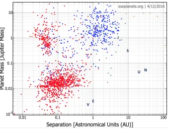
1.1 A plot of all known exoplanets, shown in mass and separation. The points are colored

by discovery method: red is transits, blue is radial velocities, green is microlensing, and

yellow is direct imaging. (Astrometry has not discovered any planets.) Solar system

planets Venus, Earth, Jupiter, Saturn, Uranus, and Neptune are shown as letters. Error

bars are omitted for clarity. This plot was generated from the exoplanet orbit database

at www.exoplanets.org. . . 2

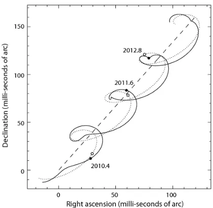
1.2 The apparent path on the sky of a star orbited by a 15 Jupiter mass planet in an

elliptical (e = 0.2) orbit of semi-major axis 0.6 AU, observed from the Earth. The

straight dashed line is the path of the system’s barycenter, with a proper motion of

50 mas/yr. The dotted line is the parallactic path of the system, with the looping

behavior due the apparent motion of the star against background stars due to the orbit

of the Earth around the Sun. The solid line shows the photocenter motion due to the

orbiting planet, with the perturbation increased by a factor of 30 to make the effect

visible. This figure is taken from Perryman (2011). . . 3

1.3 The transit probability can be calculated as the solid angle of the stellar diameter

rotated about the orbital axis. See the text for details. . . 7

1.4 The relation between various angles relevant in gravitational microlensing. See the text

for details. This figure is taken from Gaudi (2010). . . 10

1.5 An example of a microlensing light curve. The large “main” magnification event of∼2 magnitudes, or a factor of 6.3 in brightness, corresponds to the lens star, and is well

described by Equation 1.15. The small perturbation at the 5% level corresponds to

the planet around the M-dwarf lens star, a 5.5 M⊕ cool Super-Earth at a ∼2.6 AU separation. Different colored points correspond to different observatories. This figure

is taken from Beaulieu et al. (2006) . . . 11

1.6 A Keplerian elliptical orbit (see Table 1.3.2.1). The reference direction is generally

north (i.e., towards the orbital axis of the Earth), the reference plane is the plane of

(17)

1.7 An example of a radial velocity measurement at about the current limit of precision

of 1-2 m/s, taken from the HARPS spectrograph (Mortier et al., 2016). (a) Radial

velocities of the star HD175607 are measured over a significant time period. Note the

x-axis of the top curve is in days, corresponding to nearly ten years of observations.

The red curve shows the model fit, with the rapid variations due to the inner planet and

the slow variations to a potential outer companion (b) The phase-folded light curves

and fits of the signals, corresponding to periods of 29 days (top) and 1400 days (bottom). 17

1.8 A fake spectrum of a star, with a deep absorption line and a shallow, broad absorption

line. The x-axis is in wavelength, and the y-axis is in flux, both in arbitrary units.

The pixels of the spectrum corresponding to the deep line have high quality Doppler

information (red shading); the pixels of the shallow line have relatively poor quality

Doppler content. The pixels of the continuum have no Doppler information whatsoever.

This is equivalent to saying that it is impossible to determine the translation of a

function of the typey= constant. . . 20

1.9 Modal noise: The end of a fiber has two slightly different intensity distributions for

two different wavelengths (top). The addition of a slit exacerbates the differences (top

middle). The two slits are imaged as resolution elements onto the detector by the

spec-trograph. The detector spectrum has spatial variations in the cross dispersion direction

as a function of wavelength(bottom middle). The extracted spectrum (summed in the vertical direction) has quasi-periodic variations in the continuum intensity (bottom) . 23

1.10 (Left) An image of the Sun’s surface, showing spots and convective granulation, with

the Earth to scale.1_{(Right) An example of a radial velocity signal induced by a starspot.}

In this figure, the left part of the star is rotating towards the reader. As the spot rotates

into view, following the stellar rotation period, a redshift is recorded. After the star

crosses the center, a blueshift is recorded. For more complicated starspot paths, the

signal would change in complex ways. This figure is taken from Dumusque et al. (2011a) 25

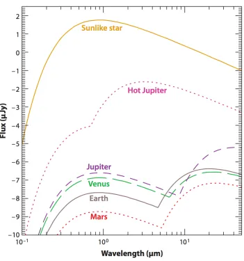
1.11 The flux of light from a sun-like star compared to various planets in the solar system,

and a hypothetical hot Jupiter. All these are blackbody curves; real planets and stars

have more complicated spectra, but the approximations are quite accurate for the

continuum levels. Note that the shorter, visible wavelengths are all reflected light

and track the spectrum of the star, while the longer infrared wavelengths are thermal

emission and are somewhat larger. The contrast between the Earth and the Sun is ten

(18)

1.12 A simulation of the formation of Jupiter, showing the growth in mass and radius as a

function of time. Mass grows slowly until the core reaches about 10 Earth masses, at

which point runaway gas accretion occurs and the radius contracts rapidly. This figure

is taken from Lissauer et al. (2009) . . . 32

1.13 A numerical hydrodynamics simulation showing the fragmentation of a protoplanetary

disk very far from the central star. The figure is taken from Boley (2009). . . 33

1.14 The evolution of effective temperature and radius of a planet as a function of age,

plotted for different mass planets. Note the much higher initial temperature and radii

due to the disk instability formation scenario (“hot start”) vs the core accretion (“cold

start”) scenario. The effects of planet formation mechanism vanish after a few hundred

million years. This figure is taken from Spiegel & Burrows (2012). . . 34

1.15 The evolution of flux in mJy as a function of wavelength, for different ages, for the

disk instability (“hot start”, red curves) scenario, and the core accretion (“cold start”,

blue curves) formation mechanism. The figure on the right is for a 1 Jupiter mass

planet, the one on the right for a 10 Jupiter mass planet. Each curve is an isochrone

corresponding to 1, 3, 10, 30, and 100 million year ages, with the younger ages having

brighter fluxes. Note the different vertical scales on the left and right figure. The black

lines at the top correspond to the J, H, K, L, M, and N infrared bands. This figure is

taken from Spiegel & Burrows (2012). . . 34

1.16 The contrast of various planets compared to a Sun-like star, as a function of

wave-length. The red and light blue curves show models similar to those presented in Figure

1.15; three known exoplanets are shown at the top. Jupiter, in pink, is shown at the

bottom. Note that the relative contrast seems to reach a peak at around 3.5 - 5 microns,

corresponding to the infraredL0andM0bands. This figure is taken from Skemer et al.

(2014) . . . 35

1.17 Basic operation of a Lyot coronagraph. The star is brought to focus and blocked by a

focal plane mask. A second stop in a pupil plane (the Lyot stop, slightly smaller than

the pupil) blocks starlight that is diffracted around the focal plane mask, and a camera

brings the remaining light to a focus. For a planet near the star (red light, bottom

panel), the planet is focused near, but not on, the first disk, since it is separated on

the sky, and is not affected by the Lyot stop. In this design, a simple Lyot

corona-graph can block about 99% of the stars light while allowing the planets light to pass

through unaffected. (This image was generated from a combination of images from the

www.Lyot.org website) . . . 37

1.18 A one dimensional coronagraph. See the text for details. This figure is taken from

(19)

1.19 A plot of the top contrasts achieved by various modern coronagraph designs, plotted in

inner working angle—bandwidth space. Note some coronagraphs show up more than

once if measurements were performed at more than one bandwidth. Contrast levels

correspond to the size of the circles. For a description of the coronagraphs, see Table

1.4.3.1. These are empirical results, and are slightly out of date as of this writing. This

figure is taken from Mawet et al. (2012) . . . 42

1.20 The planetary and zodiacal light levels for a Solar system twin at 10 pc, as viewed with

a 2m and 8m class telescope. An Earth twin is shown on the left, with a Jupiter twin

on the right. The zodiacal light can dominate the light at the infrared, but visible is

more amenable, particularly with a larger telescope. Compare the spectral features to

Figure 1.11. This figure is taken from Kasting et al. (2009), in the Decadal review of

Astronomy. . . 43

1.21 A sinusoidal phase ripple in the pupil plane will form two speckles in the image plane.

This is real image data, not simulated, and was taken from (Martinache et al., 2014) . 45

1.22 Raw images from Project 1640, the Gemini Planet Imager, and SPHERE, all showing

large amounts of speckle noise. Images from the respective project websites. . . 45

1.23 A cartoon of angular differential imaging. The planet (red) appears at different

po-sitions in the focal plane at different observing times due to sky rotation. A median

frame contains the speckle light, but not the planet. This median is subtracted from

all the individual data frames, which are then derotated and combined to reveal the

planet. This image was taken from www.astrobites.org. . . 46

2.1 Doppler precision as a function of wavelength range and star temperature for a fixed amount of observing time (60 s). The stellar spectra are derived from rotationally-broadened main-sequence templates from 2600-6200K, stepped in 200K increments,

and the wavelength range is stepped in 100 nm increments. The contours indicate the

velocity precision in m/s. From the perspective of velocity precision, the best result is

achieved in the range of 400-600 nm. The hashed regions correspond to wavelengths

where the infrared absorption is too high for ground-based observations to be effective.

This simulation assumes a 1.28 m2 _{telescope dish, a spectrograph with}_R_{=75000, and}

sky-to-detector throughput of 10% (the full simulation parameters, including stellar

(20)

2.2 The time (seconds) to detect (σv =K) a planet withMpla−

1/2

pl = 5M⊕(1AU)

−1/2_{, 10}

parsecs away, for a range of observing wavelengths and stellar effective temperatures.

The hashed regions correspond to wavelengths where the infrared absorption is too

high for ground-based observations to be effective. This simulation assumes a 1.28 m2 telescope dish, a spectrograph withR=75000, and sky-to-detector throughput of 10%

(the full simulation parameters, including stellar parameters, are given in the Appendix). 64

2.3 The maximum number of observable stars each night, with the goal of achieving the

velocity precision necessary for a detection of a planet withMpla

1/2

pl = 5M⊕AU

1/2 _on

each star. This is plotted as a function of observing wavelengths, assuming 9 hours of

observing time per night and 2 minute acquisition time between targets. The survey

was simulated using the RECONS 7 pc sample and the present-day mass function (Reid

et al., 2002), and extends to 20 pc (going out to 300 pc makes little difference, as bright

and nearby stars are the most time-efficient targets). . . 64

2.4 The time (seconds) to detect (σv = K) a 5 M⊕ planet in the habitable zone of its

parent star, 10 parsecs away, for a range of observing wavelengths and stellar

effec-tive temperatures. The hashed regions correspond to wavelengths where the infrared

absorption is too high for ground-based observations to be effective. This simulation

assumes a 1.28 m2 _{telescope dish, a spectrograph with}_R_{=75000, and sky-to-detector}

throughput of 10% (The full simulation parameters, including stellar parameters, are

given in the Appendix). . . 66

2.5 The maximum number of observable stars each night, with the goal of achieving the

velocity precision necessary for a detection of a 5 M⊕ habitable-zone planet on each

star. This is plotted as a function of observing wavelengths, assuming 9 hours of

observing time per night and 2 minute acquisition time between targets. The survey

was simulated using the RECONS 7 pc sample and the present-day mass function (Reid

et al., 2002), and extends to 20 pc (going out to 300 pc makes little difference, as bright

and nearby stars are the most time-efficient targets). . . 67

2.6 The resulting velocity precision and signal-to-noise ratio for an observation of a

Sun-like star with varying resolution, (3.0 samples/resolution element). Note that the units

on the vertical axis are m/s for the blue curve (velocity precision), and unitless for the

red curve (signal-to-noise ratio). The exposure time is held fixed, and the resulting

signal-to-noise ratio decreases as resolution increases, since less photons are incident per pixel. Increasing the resolution always improves the velocity precision, but the

point of diminishing returns is reached at about R = 45,000, which corresponds to the

(21)

2.7 The resulting velocity precision for observation of a Sun-like star with R=75000 (3.0

samples/resolution element), and skewness varying from 10−1 _{to 10}−4_{. For reference,}

the inset shows a gaussian with skewness (notα) of 0.3, an order of magnitude higher

than the maximum value considered (none of the skew-normal distributions simulated

have skews large enough to be visually distinct from a normal distribution.) The

skewness sets a signal-to-noise floor when it is greater than a part in 100, weakly

dependent on signal to noise. The flattening out of the curves occurs where the

signal-to-noise ratio limits the velocity precision. . . 72

2.8 The resulting velocity precision for observation of a Sun-like star with R=75000 (3.0

samples/resolution element), and perturbation amplitude varying from 10−4 _{to 10}−1

of the peak amplitude of the LSF. For comparison, the inset shows a gaussian with a

perturbation of 10%, equal to the maximum value considered. It is clear that for sub

meter/sec precision, it is important that the perturbation amplitude of the distribution

does not exceed 0.1 %, a value weakly dependent on the signal-to-noise ratio. The

flattening out of the curves occurs where the signal-to-noise ratio limits the velocity

precision. . . 73

2.9 The maximum number of observable stars as a function of observing wavelengths,

assuming 9 hours of observing time per night and 2 minute acquisition time between

targets. The survey was simulated using the RECONS 7 pc sample and the present-day

mass function (Reid et al., 2002), and extends to 20 pc (going out to 300 pc makes little

difference, as bright and nearby stars are the most time-efficient targets). This graph

assumes a survey targeting habitable zone planets, with velocity precisions limited to

0.5 (top), 1, 3, and 5 m/s. Furthermore, the region of 0.7-0.8µm is the best area to

observe overall. . . 74

3.1 The required integration time per night for the MINERVA array to detect 3 Earth-mass

planets within the habitable zones of each star in theη⊕sample according to a photon

limited noise model as a function ofV magnitude. Data points are colored according

to their effective temperatures, determined using stellar masses from Howard et al.

(2010b). This figure appears in Swift et al. (2015). . . 82

3.2 The differences in cost of telescopes of different aperture diameters. Commercial

(am-ateur) telescopes are shown in red, professional telescopes are shown in blue. The

CDK-700s (the telescopes we eventually chose) are shown as green points. This figure

(22)

3.3 The location of our test site at Caltech, with the first two telescopes visible. The

astronomy department is in the orange building across California boulevard at the top

left. . . 86

3.4 Engineering drawing of a modified Aqawan with two CDK-700 telescopes inside (see

next section, compare to Figure 3.3). . . 87

3.5 CDK700 telescope in our Aqawan enclosure in Pasadena. The telescope is positioned

in its neutral position, pointing south at about 30 degrees. Also visible is the Andor

iKonL camera, guider, and filter wheel on one of the ports. . . 89

3.6 A single measurement of the pointing precision of the CDK-700 telescope. Each

data-point corresponds to the radial offset of the center pixel taken at 45 second intervals.

The telescope holds the star position to 2 arc-seconds over a 50 minute interval, better

than the claimed level from the manufacturer. For reference, the fiber size on the sky

and required level of pointing precision for negligible throughput loss are shown above.

It is clear that while excellent, the pointing precision is not good enough for open-loop

control. . . 91

3.7 Left: Manufacturer-supplied transmission curves for the telescope mirrors, lenses,

fil-ters, and camera quantum efficiency. Right: throughput measurements of the

tele-scope. The high level of variability is primarily due to the high level of variability in

the atmospheric conditions in the areas where the tests were performed. The derived

efficiency of 70% is in line with expectations, especially as the derived extinction of

0.25 mags/airmass is a reasonable value in the V band. These figures appear in Swift

et al. (2015). . . 93

3.8 Left: Optical layout of the fiber acquisition unit. The primary beam path (top to

bottom) couples light from the telescope into the fiber. The second path (top to left)

images the star onto a guide camera. The third path (bottom to right to left) images

the fiber tip onto the detector. Right: mechanical drawing of the FAU; fiber tip to

base is about 8 inches long. . . 95

3.9 Fiber acquisition unit mounted on a CDK-700 telescope in the Pasadena Aqawan. The

different subcomponents are labeled, including the fiber used to make the throughput

measurements. This figure appears in Swift et al. (2015). . . 96

3.10 Thorlabs BP108 pellicle transmission for different polarization states. This image was

taken from the manufacturer website. . . 97

3.11 Left: Theoretical throughput including pellicle transmission (PT), reflection (ηR),

ge-ometric fiber injection (ηin), and fiber transmission (ηthru) loss, for a range of seeing

values. Right: Numerical simulation of geometric injection efficiency for a range of

(23)

3.12 (Left) Raw pixel tracking data with the closed loop guiding on (shaded region) and

off. The two curves correspond to thexandy pixel positions on the guider CCD. The

pitch is 0.33 arc seconds per pixel. (Right) The amplitude spectral density of the guider

error is smaller at essentially all frequencies when guiding, especially low frequencies

corresponding to long-term drifts. The intersection of the green (guiding) curve with

0 at 0 Hz indicates there is no systematic error. . . 106

3.13 The focused image of a star on the guide camera, and the diverging output beam of

the fiber. The region of relatively reduced flux in the center of the fiber image is due

to the effects of focal ratio degradation. . . 107

3.14 A throughput measurement in typical Pasadena seeing conditions of∼2”. The efficiency is about 50% (45% throughput), in line with the expectations of Figure 3.11. The

statistical deviation about the mean is 1.5% (absolute), which is smaller than our

systematic error. . . 107

3.15 Photometric camera optical setup, with major subcomponents labeled. This figure

appears in Swift et al. (2015). . . 108

3.16 Photometric time series of 16 Cygnus A and B; data binned to one-minute intervals.

The photometry is quite stable with little evidence of residual correlated noise. This

figure appears in Swift et al. (2015). . . 108

3.17 Allan deviation of the photometric light curve of 16 Cygnus A, showing a precision

of 1 mmag reached in about 3 minutes, almost at the photon noise limit. This figure

appears in Swift et al. (2015). . . 109

3.18 The final location of MINERVA, at Mt Hopkins, Arizona. The building to the

immedi-ate North of the two Aqawans is the now repurposed VERITAS observing station; the

VERITAS dish has already been removed. The HATNet and MEarth observatories are

labeled to the North. A scalebar is shown to the bottom right. The geographic

coordi-nates of this location are 31◦ 40’ 49.1”N, 110◦ 52’ 44.6” W. This image was generated

using Google Maps. . . 110

3.19 MINERVA installed at Mt. Hopkins. This photo was taken right after the four

tele-scopes were installed. The clamshell dome in the bottom right is a sister project called

MINERVA-RED (PI: Cullen Blake) . . . 111

4.1 The basic vortex coronagraph. Light from a clear telescope pupil (bottom row) is

focused on the vortex by the telescope optics. At the following pupil, the starlight is

moved to outside the pupil, where it is blocked by a Lyot stop. The dark pupil is then

reimaged by the camera, with the starlight removed. For a centrally obscured aperture

(24)

4.2 The ring-apodized vortex coronagraph apodizes the input pupil of the telescope, with

the result being that in the pupil plane after the vortex, all the energy inside the pupil

is localized to a ring (second square panel, top). A pupil stop can effectively block this

light and thus have total starlight cancellation in principle. . . 118

4.3 Schematic of the dual-vortex coronagraph. The first vortex leaves a residual halo of

light (4th panel from left) which is moved behind the pupil by the second vortex (2nd

panel from right). . . 119

4.4 The SDC mounts between the P3K adaptive optics system (blue rectangle, left) and

infrared imager PHARO (partially visible behind its red electronics box). The imager,

coronagraph and adaptive optics system all attach to Cassegrain port of the telescope. 120

4.5 The optomechanical layout of the SDC; refer to the text for a more detailed description.

Following the input beam from the top right of the figure: first fold mirror, dichroic

beam splitter, linear coronagraphic slide, off-axis paraboloid, fold mirror, Lyot plane,

fold mirror, off-axis paraboloid, linear coronagraphic slide, off-axis paraboloid, Lyot

plane, off-axis paraboloid, fold mirror. The infrared tracker is the green square. The

image and pupil viewing camera and lenses are shown on the left, directly below the

first off-axis paraboloid. In this orientation, the output beam to the infrared imager

PHARO exits downward into the page. . . 121

4.6 Coronagraphic speckle nulling in the dual-vortex mode using the internal white light

source of the adaptive optics system; see 4.4.1.2. (a) The initial results of PSF

cor-rection using MGS (4.4.1.1) still leaves many residual speckles in the focal plane. (b)

Four iterations of speckle nulling remove most of the residual wavefront errors (c) Nine

iterations get to within a factor of two of the detector read noise from 5 - 25λ/D. The

white polygon demarcates the control region, which is selected by mouse clicks in the

half-region control mode. (d) Contrast improvement measured in the control region

shows factors of 3-6 improvement, which are significant for companion detectability.

The contrast curve is defined in the usual way, with the standard deviation (ie, 1σ) of

surface brightness at each radial separation being used to generate the curve, and

nor-malized by dividing by the peak flux of the non-coronagraphic PSF (not shown). The

background limit is determined by the contrast in a region of the detector 100’s ofλ/D

away. The preprocessing steps performed on the data only consist of dark subtraction

and flat-fielding. . . 124

(25)

4.8 Laboratory contrast measurement comparing single (dashed curve) and dual vortex

mode (solid curve). The contrast curve is defined in the usual way, with the standard

deviation (ie, 1σ) of surface brightness at each radial separation being used to generate

the curve, and normalized by dividing by the peak flux of the non-coronagraphic PSF

(not shown). The preprocessing steps performed on the data only consist of dark

subtraction and flat-fielding. . . 128

4.9 (a) Raw contrast measurement with the ring-apodized vortex coronagraph. The

con-trast curve is defined in the usual way, with the standard deviation (ie, 1σ) of surface

brightness at each radial separation being used to generate the curve, and normalized

by dividing by the peak flux of the non-coronagraphic PSF (not shown). The

prepro-cessing steps performed on the data only consist of dark subtraction and flat-fielding.

(b) The coronagraphic (top) and non-coronagraphic PSF, shown on different

logarith-mic scales to enhance features. (c) The measurement of the output pupil intensity

corresponds well to theoretical expectations, with the major discrepancy being outside

the pupil. This is due to the presence of an chromium dot in the center of the vortex,

reducing stellar leakage. The center of the PSF is the brightest, so light blocked there

will not show up outside the pupil. . . 130

4.10 A reduced image of one of our target stars (K=8, V=6) with the associated 5σ

con-trast curve on the right. The reduction strategy used was a zonal principal components

analysis (KLIP) algorithm (see Section 4.4.3), with the principal components generated

from a calibrator star with similar brightness andV−Kcolor. The total open shutter time on this target was 14 minutes, with the same time on the calibrator star

(back-grounds, flats, and non-coronagraphic PSF frames were recorded separately). This

measurement did not involve speckle nulling, so contrast at small angles can likely be

improved further in the future. . . 131

4.11 Epsilon Cephei b. (a) The original discovery image, from Mawet et al 2011 (Mawet

et al., 2011a), using a 1.5 m well-corrected subaperture of the Hale telescope. (b) Raw

(no reference subtraction) SDC image, dual vortex mode, 15s of 10 median combined

frames. (c) Classic PSF subtraction of (b). In the SDC images, the first Airy ring is

visible around the companion. . . 132

4.12 The PSF-subtracted coronagraphic image of delta Andromeda b, dual vortex mode.

(26)

5.1 Left: a) the background-subtracted target median image, b) the background-subtracted

reference star median image, c) the background-subtracted point-spread function

im-age, d) best-fitting model from the MCMC algorithm combining images b) and c) and

attempting to match a) as explained above. The stretch is nonlinear to better show

the companion and speckles. Right: All the one and two dimensional projections of the

posterior probability distributions of the pixel shifts (xc,yc, the reference background

scaling factor (Ra, and the PSF amplitude used to fit the companion Pa. The

two-dimensional projections show very little covariance among any two parameters, and

the marginal distribution histograms (along the diagonal) are nicely peaked. . . 140

5.2 The reduced, background-removed coronagraphic image of δAndromedae. The first

Airy ring is visible around the companion. The stretch in the image is linear. The

colorbar shows the relative intensity (as a fraction) compared to the primary . . . 141

5.3 Comparison of the approximate fluxes ofδAnd A, three K dwarfs, and a 50000K white

dwarf. The spectral models are from Castelli & Kurucz (2004). The grey bar shows

the span of the Bracket-γ filter. . . 142

6.1 Complex plane representation of speckle phasors. A speckle at positionsλ/x0

contain-ing phase-type (orange arrows) and amplitude-type (red arrows) contributions with

electric field phases π/2±α and π±β, respectively, where α and β are the pupil phases. The dashed arrows refer to the components at−λ/x0, and the solid arrows

refer to the components atλ/x0. A speckle atλ/x0may be nulled out by the electric

field phasor corresponding to the blue dashed arrow (as can be seen by computing the

phasor sums when lying the arrows head to tail). This will not simultaneously null out

(27)

6.2 Coronagraphic speckle nulling in the dual-vortex mode using the internal white light

source of the adaptive optics system. The value of λ/D is ∼ 90 mas (a) The initial results of PSF correction using MGS still leaves many residual speckles in the focal

plane. (b) Four iterations of speckle nulling remove most of the residual wavefront

errors (c) Nine iterations get to within a factor of two of the detector read noise from

5 - 25 λ/D. The white polygon demarcates the control region, which is selected by

mouse clicks in the half-region control mode. (d) Contrast improvement measured in

the control region shows factors of 3-6 improvement, which are significant for

compan-ion detectability. The contrast curve is defined in the usual way, with the standard

deviation (i.e., 1σ) of surface brightness at each radial separation being used to

gen-erate the curve, and normalized by dividing by the peak flux of the non-coronagraphic

PSF (not shown). The background limit is determined by the contrast in a region of

the detector 100’s ofλ/D away. The preprocessing steps performed on the data only

consist of dark subtraction and flat-fielding. . . 159

6.3 Non-coronagraphic speckle nulling with the instrument TMAS using the internal white

light source of the adaptive optics system. The value of λ/D is ∼ 30 mas. (a) The initial results of PSF correction using Zernike tuning leaves many speckle aberrations

in the focal plane. (b) Four iterations of speckle nulling. (c) Nine iterations of speckle

nulling. The contrast improvement in this case is a modest 20-40%, but could possibly

have been increased by running for more iterations (at the time this experiment was

performed, the control software did not provide automatic feedback about the contrast

improvement, so we were not aware that there was much more improvement to be

had). Some of the limitations here are due to the starting level of aberrations being

far higher than in the longer-wavelength instruments, as described in the text. It is

encouraging to note that more of the diffraction pattern is visible in the last image than

in the first. The contrast curve is defined in the usual way, with the standard deviation

(i.e., 1 σ) of surface brightness at each radial separation being used to generate the

curve, and normalized by dividing by the peak flux of the non-coronagraphic PSF. The

(28)

6.4 Coronagraphic speckle nulling in L-band on NIRC2, using the internal white light

source of the adaptive optics system. The value of λ/D is ∼80 mas. (a) The initial results of PSF correction using image sharpening leaves many speckle aberrations in the

focal plane. (b) Four iterations of speckle nulling. (c) Nine iterations of speckle nulling.

The white lines demarcate the control region, with the outer line at approximately the

limit of the control bandwidth of the deformable mirror. The contrast improvement

in this case is a factor of 5-10, and gets within a factor of 2-3 of the background

limit. The contrast curve is defined in the usual way, with the standard deviation

(ie, 1 σ) of surface brightness at each radial separation being used to generate the

curve, and normalized by dividing by the peak flux of the non-coronagraphic PSF. The

and flat-fielding. . . 163

7.1 Schematic of the dual-vortex coronagraph. The first vortex leaves a residual halo of

light (4th panel from left) which is moved behind the pupil by the second vortex (2nd

panel from right). In the second pupil plane, this light can be blocked, creating an

effective conventional coronagraph. Alternatively, it can be picked off and used as a

“reference” beam, as we do here with a phase-shifting mirror, described below. This

figure originally appeared in Bottom et al. 2016 . . . 173

7.2 (a) Mechanical drawing of the phase shifter mount. The piezoelectric flexure stage

is shown in dark grey, the interface to the annular mirror mount is in pink, and the

annular mirror mount is in yellow. The annular mirror mount is actuated on the three

axes, but the actuators are omitted for clarity. The mirrors are shown in blue. (b)

Cutaway of the phase-shifter assembly, showing the hardware to align the rod to the

mirror and the direction of travel of the rod. The mechanism is installed at the “Lyot

stop 2” location in Figure 7.4. . . 174

7.3 (a) The point spread function of the combined outer mirror and phaseshifting rod. (b)

The point-spread function of the inner phase-shifting rod only. The images are the

same size, with each edge spanning 6.25 arc-seconds (250 pixels). The images are not

at the same scale or exposure time, but have been individually stretched to bring out

(29)

7.4 The optomechanical layout of the SDC. Following the input beam from the top right of

the figure: first fold mirror, dichroic beam splitter, linear coronagraphic slide, off-axis

paraboloid, fold mirror, Lyot plane, fold mirror, off-axis paraboloid, linear

corona-graphic slide, off-axis paraboloid, second Lyot plane, off-axis paraboloid, fold mirror.

The infrared tracker is the green square. The image and pupil viewing camera and

lenses are shown on the left, directly below the first off-axis paraboloid. In this

orien-tation, the output beam to the infrared imager PHARO exits downward into the page.

The phase-shifter assembly is at the second Lyot plane, labeled “Lyot stop 2” in the

image. This figure originally appeared in Bottom et al. 2016 . . . 175

7.5 (a) An image is taken at each pistoning mirror position (z). The red line shows a cut

through a particular pixel, at different mirror positions. (b) Raw data of intensity (in

counts) vs mirror position for three different pixels of similar intensity in the image

plane. The relative phases between the three different waves correspond to differences

in electric field phase. . . 178

7.6 Phase sensing in the focal plane. (Top row) The left-hand plot shows the intensity

measurements in the focal plane, with diffraction spikes clearly visible. This measure

of intensity is a typical image shown on an camera. On the right, the corresponding

phase map is shown. (Bottom row) The outlined region in the top plot, magnified

to show detail. Speckles and their Airy rings are more easily identified in the phase

plot, with a 180 degree phase shift between the cores and first Airy rings. Note that

speckle chromatic effects such as elongation show themselves as phase gradients across

an individual speckle; for example, in the central speckle in the image, indicated by

the arrow, the measured phase is seen to increase from 240 to 300 degrees across it. . 179

7.7 The derived map of the phase gradient over the same area as in Figure 7.6. . . 180

7.8 Laboratory demonstration of coronagraphic speckle-suppression using the phase-shifting

interferometer. The white outline delineates the region of speckle control. Panels a,

b, and c show the intensity after 0, 4, and 9 iterations of speckle removal by the

de-formable mirror. Panels d and e show the phase measurements of the initial and final

light distribution, showing a clear difference in phase. Panel f shows the 1σ contrast

curve measurement of the region after 1, 4, and 9 iterations. The contrast curve is

defined in the usual way, with the standard deviation (ie, 1σ) of surface brightness at

each radial separation being used to generate the curve, and normalized by dividing by

the peak flux of the non-coronagraphic PSF (not shown). The preprocessing performed

(30)

7.9 Coherence modulated detection of HD 49197b. (a) The mean of the target frames.

The substellar companion is not clearly visible in the image. The companion is present

at an SNR of about 5. The stretch is logarithmic. (b) The incoherent intensity map

(Equation 7.21). The companion is easily visible at a position angle of about 275

degrees, and has an SNR of about 7.5. The stretch is also logarithmic. We note that

the same data frames were used to compute image (b) as in (a), except combined using

the interferometer position to give extra information. No reference star is used. (c)

Principle components analysis (KLIP) reduction of HD49197b, where the components

are generated from only the coherent parts of the image data, as explained in Section

7.5.2. No reference star is used, and the SNR is 9. The stretch is linear. (d) A

conventional PSF-subtracted image of the companion, using a nearby reference star,

(31)

List of Tables

1.1 Summary of coronagraphs presented in Figure 1.19. . . 41

3.1 CDK-700 optical, mechanical, electronic, and pointing parameters, as specified by the

manufacturer Planewave Instruments. . . 90

3.2 Equation terms for determining telescope throughput . . . 92

3.3 Andor iKon-L parameters and filters . . . 103

4.1 The different on-sky observing modes of SDC; see section 4.2 for a description of each

of these modes. . . 127

4.2 The actuated optics in the SDC, their degrees of freedom, and the optical fields they

control. Refer to Figure 7.4 for the an optical layout . . . 134

4.3 List of optics, electronics, and related information . . . 134

5.1 Previously measured properties ofδAnd and newly measured properties of the companion137

5.2 Summary of observations. . . 138

7.1 Summary of reductions. All observations of HD 49197 and reference star HD 48270

(32)

Chapter 1

Introduction

1.1 Overview of methods of exoplanet detection

The major methods of detecting extrasolar planets are astrometry, transits, gravitational

microlens-ing, radial velocities, and direct imaging. These are the only ways that have either detected many

planets, or at least have the hope of detecting many planets. Each method has its advantages and

disadvantages, and none can by itself explore the full diversity of planetary systems. A plot of all

currently confirmed exoplanets is shown in Figure 1.1.

In the following sections, we present these different ways of detecting extrasolar planets, giving a

basic introduction to the physical principles behind the methods, their sensitivities, and their range

of applicability. We will take a “signals analysis” perspective, focusing on the frequency, amplitude,

and noise sources of planet signals. We believe this is the most useful way to understand exoplanet

science for experimental detection work. For a tabular comparison of methods, see Table 1.2.1.

We split the presentation into a few parts. First, we present a short overview of astrometry,

transits, and microlensing, which are not very relevant to the work in this thesis, but useful for

having a general picture of the current state of the field and its future. For these three methods, we

draw heavily from Perryman (2011) and Seager (2010). We then devote one section each to radial

velocities and direct imaging, the methods used in this thesis, in much more detail. The reader who

is only interested in the work on radial velocities or direct imaging in this thesis might consider

reading those respective sections, though background is provided in each chapter. The reader who

(33)

[image:33.612.155.495.231.493.2]

(34)

[image:34.612.216.432.241.452.2]

(35)

4 frequency Duration Radial velocity Stellar line shift/velocity

v= 9.8P

1yr

−1 3_M

psini M⊕

Ms

M

−2 3

cm/s

∆λ λ =

v c

∆λ λ = 10

−8 _(Jupiter)

∆λ λ = 10

−10_(Earth)

Orbital period,

days to decades

Always Always, but high

incli-nation angles

problem-atic

Transit Stellar

inten-sity decrement

∆f=

_R

p

R∗

2

∆f≈10−2 _{(Jupiter, Sun)}

∆f≈10−4 _{(Earth, Sun)}

Orbital period,

days to decades

Hours P= R∗/a, typically <

1%

Astrometry Stellar

photo-center shift α= _M p M∗ a 1AU d 1pc −1

arcsecond α≈5·10−4_{” (Jupiter, Sun,}

d=10 pc)

α≈3·10−7_{” (Earth, Sun,}

d=10 pc)

Orbital period,

days to decades

Always Always

Microlensing Background

star intensity

perturbation

Complex, but very weakly dependent on

planet mass(!)

∆Mag

Mag >0.05 None,

single-shot

observa-tion

Few hours to

few days

10−6 events/star/yr

near galactic bulge

Direct

imaging

Planet light fp(φ,λ)

f∗(λ) =A(λ)

_R

p

a 2

g(φ) (reflected)

fp=πR2pB(λ, Tp) (self luminous)

fp

f∗ ≈ 10

−10 _{(Earth, Sun}

visible to near-IR)

fp

f∗ ≈ 10

−8 _{(Jupiter, Sun}

visible to near-IR)

0,

Non-temporal

signal

(36)

1.2 Astrometry, Transits, and Microlensing

1.2.1 Astrometry

The astrometric method of discovering planets is one of the oldest, and was the most heavily pursued

methods up until the relatively recent past, likely due to its prolific results with binary stars. The

principle of the astrometric discovery method is to look for small, periodic changes in the position of

a star caused by unseen orbiting companions. By measuring many points of the angular deviation of

the star against the plane of the sky, in particular nearby reference stars, the presence of a companion

may be inferred, and all 7 Keplerian orbital elements can be determined. Since the center of mass

in a system governed by gravitational forces is stationary, a planet and its host star will both orbit

their (fixed) barycenter. In that case, the center of mass of the star will trace out an ellipse of

semi-major axis

a∗=

Mp

M∗

ap (1.1)

where arefers to the semi-major axis of the orbit. The units of a∗ are physical lengths; in reality,

what is measured is an angular motion in the plane of the sky, which depends on the distance to

the star. These two quantities may be related via the definition of the parsec, as

α= Mp M∗

ap

d =

_G

4π2

13 _M

p

M∗2/3

P2/3

d (1.2)

= 3µasMp M⊕

M∗ M

−2/3

P 1yr

2/3

d 1pc

−1

(1.3)

where the second equality follows from Kepler’s laws (see Section 1.3.2.1), relating the semi-major

axis of the planet’s orbit to the period, with the approximation that Mp << M∗. From this

equation, it can be seen that an Earth-like planet at 10 parsecs away would give a signal of about

3·10−7 arcseconds, or 0.3 µas. In order to measure this signal, or course, multiple epochs would have to be observed. The fundamental, shot-noise limited accuracy as to how well a telescope can

measure a position is determined by the angular resolution and signal to noise ratio in a simple way

(Lindegren, 1978):

σph=

λ 4πD

1

SNR (1.4)

where D is the dish diameter, but almost no telescopes on the ground approach this limit due

to the deleterious effects of atmospheric turbulence. It should also be pointed out that Equation

1.4 scales, at best, as the square root of the exposure time, as given by the Poisson statistics of

(37)

as long an observation. The limit from the ground achieved so far appears to be around 100µas in

optical and near-infrared frequencies (Cameron et al., 2009), with some groups claiming a precision

of 30µas. These observations all use adaptive optics to sharpen the point-spread functions of the

stars, and are thus limited in reference stars by the size of the “isoplanatic patch”; that is, the area

of sky which can be well corrected by the adaptive optics system. Space telescopes have better

accuracy, with Hubble being able to achieve∼30µas in drift scanning mode (J. MacKenty, private communication). Radio interferometers currently lead, with long-baseline setups achieving about 10

µas (Reid & Honma, 2014). (The D term in the equation above is replaced by the baseline of the

interferometer separation, and the scale factor is slightly modified as well.)

The astrometric method has some useful features. It is one of the few methods where more

distant planets give a stronger signal, though the time needed to make such a measurement is on

the order of the orbital period, which mostly negates this advantage. Also, it has no fundamental

“blind” spots; with a sufficiently accurate instrument, and enough observing time, a planet cannot

“hide,” which is not the case for transits, microlensing, or sometimes radial velocities. It is the only

method that can, even in principle, directly measure masses of Earth-type planets around nearby

stars. Furthermore, it measures all the Keplerian orbital parameters directly, and may be used to

derive a dynamical mass for the planet. Astrometric measurements may also be used to efficiently

break the degeneracy between mass and inclination angle that the radial velocity method gives.

Drawbacks of the astrometric method are its reliance on the orbital period for a signal detection,

the linear decrease in signal strength with stellar distance, and the substantial technical challenges in

measuring such small photocenter shifts over long periods of time. It is currently the least successful

method of exoplanet discovery, and has no confirmed detections, and many notorious false claims

being later ruled out by follow-up observations. However, the astrometric method has a bright

future. TheGaia mission, a dedicated space telescope optimized for high-precision astrometry, is expected to discover thousands of planetary systems. The data set from this mission will enhance

our knowledge of massive, long-period planets like Jupiter and Saturn, of which almost no analogs

are currently known.

1.2.2 Transits

The transit method detects planets by measuring the dip in starlight when a planet passes in front

of its parent star. It is by far the most successful method used to discover planets, with theKepler

spacecraft having found thousands of planets, ranging from sizes of smaller than Earth to larger than

Jupiter. Transiting exoplanets have revolutionized the field, allowing detailed statistical analyses of

exoplanet populations and demographics, including discovering “Super Earths,” planets with sizes

intermediate to Earth and Neptune, which are possibly the most common type of planet in the

(38)

Figure 1.3: The transit probability can be calculated as the solid angle of the stellar diameter rotated about the orbital axis. See the text for details.

The fundamental physics of the transit method are quite straightforward to describe. The

prob-ability of a transit event occurring can be calculated by

P(transit)≈ (2πa)(2R∗)

4πa2 (1.5)

= R∗

a (1.6)

= 0.005

_R

∗

R

a

1AU

−1

(1.7)

whereR∗ is the stellar radius andathe semi-major axis. The first line of the equation follows from

imagining the extreme case where a planet just touches the top or bottom of the stellar limb (see

Figure 1.3). The top and bottom of the star define the height of a cylinder of radiusawhen rotated

about all possible viewing angles. The solid angle of this cylinder is Acyl/a2, so the probability is

just this solid angle divided by the total solid angle of a sphere, 4π. (Here we are ignoring effects

like orbital eccentricity, which can somewhat boost the transit probability.) The equation shows

that the probability of detecting an Earth-like planet is about one half of one percent, and that this

does not depend on the distance to the star.

The transit depth is also possible to approximate fairly accurately. Assuming a stellar disk of

Two Roads to Planet Detection