warwick.ac.uk/lib-publications Manuscript version: Author’s Accepted Manuscript
The version presented in WRAP is the author’s accepted manuscript and may differ from the published version or Version of Record.
Persistent WRAP URL:
http://wrap.warwick.ac.uk/122225
How to cite:
Please refer to published version for the most recent bibliographic citation information. If a published version is known of, the repository item page linked to above, will contain details on accessing it.
Copyright and reuse:
The Warwick Research Archive Portal (WRAP) makes this work by researchers of the University of Warwick available open access under the following conditions.
Copyright © and all moral rights to the version of the paper presented here belong to the individual author(s) and/or other copyright owners. To the extent reasonable and
practicable the material made available in WRAP has been checked for eligibility before being made available.
Copies of full items can be used for personal research or study, educational, or not-for-profit purposes without prior permission or charge. Provided that the authors, title and full
bibliographic details are credited, a hyperlink and/or URL is given for the original metadata page and the content is not changed in any way.
Publisher’s statement:
Please refer to the repository item page, publisher’s statement section, for further information.
A New Deterministic Algorithm for Dynamic Set Cover
Sayan Bhattacharya∗ Monika Henzinger† Danupon Nanongkai‡
Abstract
We present a deterministic dynamic algorithm for maintaining a(1+)f-approximate minimum cost set cover withO(flog(Cn)/2)amortized update time, when the input set system is undergoing element insertions and deletions. Here,ndenotes the number of elements, each element appears in at mostfsets, and the cost of each set lies in the range[1/C,1]. Our result, together with that of Gupta et al. [STOC‘17], concludes a line of work on dynamic set cover: We can now obtain a deterministic algorithm for this problem withO(flog(Cn))amortized update time andO(min(logn, f))-approximation ratio, thereby matching the polynomial-time hardness of approximation for minimum set cover in the static setting. Our update time is onlyO(log(Cn))away from a trivial lower bound.
Prior to our work, the previous best approximation ratio guaranteed by deterministic algorithms was O(f2), which was due to Bhattacharya et al. [ICALP‘15]. In contrast, the only result that guaranteed
O(f)-approximation was obtained very recently by Abboud et al. [STOC‘19], who designed a dynamic algorithm with(1+)f-approximation ratio andO(f2logn/)amortized update time. Besides the extra
O(f)factor in the update time compared to our and Gupta et al.’s results, the Abboud et al. algorithm is randomized, and works only when the adversary isobliviousand the sets are unweighted (each set has the same cost).
We achieve our result via the primal-dual approach, by maintaining a fractional packing solution as a dual certificate. This approach was pursued previously by Bhattacharya et al. and Gupta et al., but not in the recent paper by Abboud et al. Unlike previous primal-dual algorithms that try to satisfy somelocal constraints for individual sets at all time, our algorithm basically waits until the dual solution changes significantlyglobally, and fixes the solution only where the fix is needed.
∗
University of Warwick, UK. Email:[email protected]
†
University of Vienna, Austria. Email:[email protected]
‡
Contents
1 Introduction 1
1.1 Technical Overview . . . 2
2 Preliminaries: Minimum Set Cover in the Static Setting 5 3 Our Dynamic Algorithm 6 3.1 A classification of elements . . . 7
3.2 The shadow input and the invariants . . . 8
3.3 The algorithm . . . 8
3.4 The REBUILD(≤k) subroutine . . . 10
4 Analysis of our dynamic algorithm 10 4.1 Bounding the update time of our dynamic algorithm . . . 12
4.2 Bounding the approximation ratio of our dynamic algorithm . . . 13
A A Static Primal-Dual Algorithm for Minimum Set Cover 17 A.1 Post-processing . . . 19
1
Introduction
In the (static) set cover problem, an algorithm is given a collection S ofm sets over a universe E ofn
elements such that∪s∈Ss = E. Each sets ∈ S has a positivecost cs. After scaling these costs by some appropriate factor, we can always get a parameterC >1such that:
1/C ≤cs ≤1for every sets∈ S. (1.1)
For anyS0 ⊆ S, letc(S0) =P
s∈S0csdenote the total cost of all the sets ins∈ S0. We say that a sets∈ S
coversan elemente∈ E iffe∈s. Our goal is to pick a collection of setsI ⊆ Swith minimum total cost
c(I)so as to cover all the elements in the universeE.
Set cover is a fundamental optimization problem that has been extensively studied in the contexts of polynomial-time approximation algorithms and online algorithms. In recent years, it has received significant attention in thedynamic algorithmscommunity as well, where the goal is to maintain a set coverI ⊆ S
of small cost efficiently under a sequence of element insertions/deletions in E. In particular, a dynamic algorithm for set cover must support the followingupdate operations.
PREPROCESS(m): Createmempty sets inS. ReturnI=∅, and identifiers (e.g., integers) to the sets inS.
INSERT(F ={s1, s2, . . .}): Insert toEa new elementewhich belongs to the setss1, s2, . . .(their identifiers
are given as parameters). Return an identifier to the new elemente, and the identifiers of sets that get added to and removed fromI.
DELETE(e): Delete elementefromE. Return the identifiers of sets that get added to and removed fromI.
After each update, the algorithm must guarantee that I is a set cover; i.e. every elemente ∈ E is in some set inI. Letf andnbe the maximum size ofF andE, respectively, over all updates. The parameter
f is known as themaximum frequency. It is usually assumed thatf, nandmare known and fixed in the beginning, but note that our algorithm does not really need this assumption.1
The performance of dynamic algorithms is mainly measured by theupdate time, the time to handle each
INSERTand DELETEoperation. Previous works on set cover focus on theamortized update time, where an
algorithm is said to have an amortized update time oftif, for anyk, the total time it spends to process the firstkupdates is at mostkt. We also consider only the amortized update time in this paper, and simply use “update time” to refer to “amortized update time”. The time for the PREPROCESS operation is called the preprocessing time. It is typically not a big concern as long as it is polynomial.2
Perspective: Since the static set cover problem is NP-complete, it is natural to consider approximation algorithms. An algorithm has an approximation ratio ofαif outputs a set coverI withc(I) ≤ α·OP T, whereOP T is cost of the optimal set cover. Since the tight approximation factors for polynomial-time static set cover algorithms areΘ(logn)andΘ(f)(e.g. [13, 12,11, 19,16]), it is natural to ask if one can also obtain these same guarantees in the dynamic setting with small update time. TheO(logn) approximation ratio was already achieved in 2017 via greedy-like techniques by Gupta et al. [14]. Their algorithm is deterministic and has O(flogn) update time. This update time is only O(logn) away from the trivial
Ω(f)lower bound – the time needed for specifying the sets that contain a given element (which is currently being inserted). A similar lower bound holds even in some settings where updates can be specified with less than f bits [1], e.g., when elements and sets are fixed in advance, and the updates are activations and deactivations of elements.3 TheO(f)approximation ratio was recently achieved by Abboud et al. [1] (improving upon the approximation factors ofO(f2)and higher by [7,14,5]). Abboud et al. show how to
1We mention that our algorithm do not really need the preprocessing step. When I
NSERT(F ={s1, s2, . . .}) is called with a new setsi, it can simply createsion the fly.
2
Our algorithm requires only linear preprocessing time.
3Abboud et al. [1] showed that, under SETH, there is no algorithm with polynomial preprocessing time andf1−δupdate time
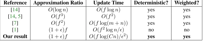
Reference Approximation Ratio Update Time Deterministic? Weighted?
[14] O(logn) O(flogn) yes yes
[14,5] O(f3) O(f2) yes yes
[7] O(f2) O(flog(m+n)) yes yes
[1] (1 +)f O(f2logn/) no no
[image:5.612.103.510.73.156.2]Our result (1 +)f O(flog(Cn)/2) yes yes
Table 1: Summary of results on dynamic set cover
maintain an(1 +)f-approximation inO(f2logn/)amortized update time. Their algorithm, however, is randomized and does not work for the weighted case (when different sets have different costs).4 Like most randomized dynamic algorithms currently existing in the literature, it works only when the future updates do not depend on the algorithm’s past output – this is also known as theoblivious adversary assumption. Removing this assumption is a central question in this area, since it may in general make many dynamic algorithms useful as subroutines inside fast static algorithms [10,18,4,3,17,8,15]. Accordingly, prior to our work, it was natural to ask if there is an efficientO(f)-approximation algorithm for dynamic set cover that isdeterministicand/or can handle theweighted case. In this paper we answer this question positively.
Theorem 1.1. We can maintain a(1 +)f-approximate minimum-cost set cover in the dynamic setting, deterministically, withO(flog(Cn)/2)amortized update time, whereCis the ratio between the maximum and minimum set costs.
Thus, we simultaneously (a) improve upon the update time of Abboud et al. [1], (b) derandomize their re-sult, and (c) extend their result to the weighted case. Our algorithm, together with the one in Gupta et al. [14], concludes a line of work on dynamic set cover [5, 7, 14, 1]. We can now get an O(min(logn, f)) -approximation using a deterministic algorithm with O(flog(Cn))update time. The approximation ratio matches the one achievable by the best possible polynomial-time static algorithm, whereas the update time is onlyO(log(Cn))away from the lower bound ofΩ(f).
1.1 Technical Overview
Previous Approaches:Theprimal-dual schemais a powerful tool for designing many static approximation algorithms. In recent years, it has also been the main driving force behinddeterministicdynamic algorithms for set cover and maximum matching (e.g. [6,9, 5,7,14]), including allO(poly(f))-approximations for dynamic set coverexcept the one by Abboud et al. [1].
Thedualof minimum set cover happens to be afractional packingproblem, which is defined as follows. Given a set system(S,E)as input, we have to assign a fractional weightw(e) ≥ 0to every element. We want to maximizeP
e∈Ew(e), subject to the following constraint: X
e∈s
w(e)≤csfor every sets∈ S. (1.2)
For the rest of this paper, we letW(s) = P
e∈sw(e)denote the total weight received by a sets∈ S from all its elements. Furthermore, definew(S) = P
e∈Sw(e) for every subset of elementsS ⊆ E. Thus, the goal is to maximizew(E)subject to the constraint thatW(s)≤csfor all setss∈ S.
4
LetOP T(S,E)denote total cost of the minimum set cover in(S,E). We simply useOP T when(S,E)
is clear from the context. All the previous primal-dual algorithms for dynamic set cover try to maintain some invariants aboutindividualsets all the time. In particular, they are based on the following lemma.
Lemma 1.2. Consider any fractional packing w in (S,E) that satisfy (1.2). Then we have w(E) ≤
OP T(S,E). In addition, if there exist a set-coverI ⊆ SofEand anα≥1such that
W(s)≥cs/αfor all setss∈ I, (1.3)
then we havec(I)≤αf·w(E)≤αf·OP T(S,E).
All the previous dynamic primal-dual algorithms maintain a set coverIand a fractional packingwthat satisfy (1.3). Needless to say, the algorithms have to change I and the weights w(e) of some elements
ein a carefully chosen manner after each update. For example, the algorithm of Bhattacharya et al. [7] satisfies (1.3) withα =O(f), implying anO(f2)-approximation factor. To obtain anO(f)approximation factor we need to satisfy (1.3) withα=O(1). However, as pointed out by Abboud et al. [1], it is not clear how to maintain such a strict constraint efficiently forα=O(1). The trouble is that one update may violate (1.3) and may cause a sequence of weight changes for many elements. This creates difficulties for bounding the update time (which typically require intricate arguments via clever potential functions).
Because of this difficulty, Abboud et al. opted for a different approach that is based on the following static algorithm. (i) Pick any uncovered elementeuniformly at random, calledpivot. (ii) Include all sets containingein the set cover solution. (iii) Repeat this process until all elements are covered. It is easy to see that this algorithm returns anf-approximation for the unweighted case (when every set has the same cost). Since this approximation ratio does not hold for the weighted case in the static setting, it seems difficult to extend the approach of Abboud et al. to the weighted case. More importantly, in the analysis of their algorithm in the dynamic setting, Abboud et al. crucially rely on randomness and the oblivious adversary assumption. This allows them to argue that before a pivot element gets deleted, many other non-pivot elements must also get deleted in expectation. Thus they can charge the time their algorithm needs in handling the deletion of a pivot to the (large number of) non-pivot elements that got deleted in the past. This type of argument was also used for maintaining a maximal matching [2,20]. To the best of our knowledge, there was no technique to derandomize this type of argument. In fact, all the known deterministic dynamic algorithms for set cover and matching use the primal-dual schema. This leads to a basic question: Is the primal-dual approach powerful enough to give anO(f)-approximation algorithm for dynamic set cover?
We answer this question in the affirmative. Unlike previous dynamic primal-dual algorithms, which try to satisfy conditions like (1.3) that arelocalto individual sets, our algorithm basically waits until the dual solution changes significantlyglobally, and then it fixes the solution only where the fix is needed.
Our Approach and the Showcase (Batch Deletion). To appreciate our main idea, consider the batch deletionsetting, where we have to preprocess a set system(S,E)and then there is an updateD ⊆ E that changes the set system to(S,E0), whereE0 =E \D. Our goal is to recompute an approximately minimum set cover in the new input(S,E0)in time proportional to the size of the update (i.e.,|D|).
Suppose that originally we have a pair (I, w)that satisfies (1.3) withα = 1 for(S,E); thus,c(I) ≤
f·w(E)≤f·OP T(S,E). Clearly,Iremains a set cover of the new set system(S,E0). To simplify things even further, suppose that the element-weights areuniform,5and|D| ≤· |E0|for some >0. This implies thatw(D)≤·w(E0). So Lemma1.2gives us:
c(I)≤f·w(E) =f · w(E0) +w(D)
≤f(1 +)·w(E0)≤f(1 +)·OP T(S,E0).
Observation 1.3. If|D| ≤· |E0|and the element-weights are uniform, thenc(I)≤f(1 +)·OP T(S,E0).
5
In words, Iremains a good approximation toOP T(S,E0)if|D|is small. Thus, intuitively we do not need to do anything when|D| ≤· |E0|. This is already different from previous primal-dual algorithms that might have to do a lot of work, since (1.3) might be violated. In contrast, when|D|becomes larger than
· |E0|, inO(f· |E0|) time we can just compute a new pair(I0, w0)satisfying (1.3) withα = 1for the set system(S,E0). Since we do this only after· |E0|deletions, we get an amortized update time ofO(f /).
One lesson from the above argument is this: Instead of trying to satisfy (1.3), we might benefit from dealing withDonly when it is large enough, for this might help us ensure that the amortized update time remains small. Of course this is easy to argue under the uniform weight assumption, which often makes the situation too simple. The following lemma is the key towards doing something similar in the general setting.
Lemma 1.4. Defines>x ={e∈s:w(e)> x}for every sets⊆ Eof elements. Suppose that:
|D>x| ≤· |E>x0 | for allx≥0. (1.4)
Then we havew(D)≤·w(E0), and thusc(I)≤f(1 +)·OP T(S,E0).
Proof sketch. Note thatw(e) = R∞
0 1(x < w(e))dx, where1(x < w(e))is one if x < w(e), and zero
otherwise. Thus, we have:
X
e∈D
w(e) = Z ∞
0 X
e∈D
1(x < w(e))dx= Z ∞
0
|{e∈D:w(e)> x}|dx= Z ∞
0
|D>x|dx
≤· Z ∞
0
|E>x0 |dx=· Z ∞
0
|{e∈ E0 :w(e)> x}|dx=·X e∈E0
w(e).
Lemma 1.4 tells us that if |D>x| ≤ · |E>x0 |for all x, then we do not have to do anything. When |D>x|> |E>x0 |for somex, we need to “fix” I. We do so by running a static algorithm on some sets and elements. The static algorithm is described in Algorithm1.5. We describe how to use it in Algorithm1.6.
Algorithm 1.5(Static uniform-increment). Given an input( ˆS,Eˆ), start withwˆ(e) ← 0for alle ∈ Eˆand
ˆ
I ← ∅. Repeat the following untilIˆcovers all elements: (i) Raise weightswˆ(e)at the same rate for every
e∈Eˆnot covered byIˆ, until some setssinS \ˆ Iˆare tight (i.e.W(s) =cs). (ii) Add such sets toIˆ. Algorithm 1.6 (Batch deletion algorithm). Initially, compute(I, w)by running Algorithm1.5 on (S,E). To handleD, letx∗be the minimumxsuch that(1.4)is violated and do the following. (Do nothing if (1.4) is not violated at all.) Run Algorithm 1.5to compute(ˆI,wˆ) for (S>x∗,E0
>x∗), whereS>x∗ = {s ∈ S :
s∩ E>x∗6=∅}. SetI ←(I \ S>x∗)∪Iˆ,D=D\D>x∗, andw(e) = ˆw(e)for alle∈ E>x∗.
In short, Algorithm 1.6 fixes I by running the static Algorithm 1.5 on input (S>x∗,E>x0 ∗). We can
implement Algorithm1.5inO(|S>x∗|+|E0
>x∗|) =O(f|E>x∗|) =O(f|D>x∗|/)time approximately.6 This
gives an amortized update time ofO(f /), since we canchargetheO(f|D>x∗|/)time spent in “fixing”I
to the elements inD>x∗that got deleted. The lemma below implies the correctness of this strategy.
Lemma 1.7. (i) Let(I, w)denote the output of Algorithm1.5when given(S,E)as input. For everyx≥0, the subset of elementsE \ E>xis covered byI \ S>x. (ii) After processingD, Algorithm1.6producesD,I, andwthat satisfy(1.4); which implies thatc(I)≤(1 +)f ·OP T(E0).
Proof Idea. For (i), Algorithm (1.5) stops raising the weight of some elemente∈ E \ E>xonly when some set s containing eis tight. At this point we also stop raising the weight of every element in s, making
s ∈ I \ S>x. For (ii), an intuition is that Algorithm1.6has subtracted fromDallD>x that violate (1.4). This subtraction does not increaseD>xfor anyx, and, thus, does not create any new violation to (1.4).
6
We can implement an approximate version of Algorithm1.5, where element weights are in the form(1 +)ifor somei, and we say that a setsis tight ifW(s)≥cs/(1 +), increasing the approximation ratio by another(1 +)multiplicative factor. It is not
Lemma1.7(i) implies that we can add/remove to/from Isets inS>x∗ without worrying about the
cov-erage of elements inE \ E>x∗(they will be covered even when we remove all sets inS>x∗fromI).
Conse-quently, we can guarantee that after processingD, Algorithm1.6produces a setI that covers all elements. Lemma1.7(ii) immediately implies the claimed approximation guarantee. Note that it is crucial to apply our new Lemma1.4with appropriateD,I, andw, which are changed after Algorithm1.6processesD.
Note that running Algorithm1.5at the preprocessing is crucial for the correctness of Algorithm1.6, as otherwiseImight not cover all elements after Algorithm1.6finishes. In other words, Lemma1.7(i) might not be true if we replace Algorithm1.5by some other static algorithm.7 We believe that this is key that gives the running time improvement over Abboud et al.’s algorithm, since otherwise we may have to spend more time checking if other elements remain covered. (This is essentially what happened in Abboud et al.’s algorithm.) Note that Algorithm1.5 was also used in previous dynamic algorithms [5, 7,14], but to our knowledge it does not play a role in the correctness of those algorithms like in our algorithm.
One detail to mention is how Algorithm1.6findsx∗. One simple way is to round element weights to the form (1 +)i for integers i. (We refer to such i as thelevelof an element in the rest of this paper.) With this rounding, we simply have to search forO(log(Cn))different choices ofx∗, whereCis defined in Theorem1.1. The total update time amortized over deletions inDbecomesO(log(Cn) +f /).
The Fully-Dynamic Algorithm (Sketched). Extending the above algorithm to handle more deletions is rather straightforward: We include a newly deleted element toD, check forx∗, and then fix(S>x∗,E0
>x∗)
as in Algorithm1.6if such ax∗exists. Handling insertions, on the other hand, is more intricate. When an elementeis inserted, we set its weightw(e)to the maximum possible value to make some setscontaining
etight, i.e.P
e∈E∪Dw(e) =cs(note that elements inDalso contribute to the weights of sets). This means that ifeis already in a tight set, thenw(e) = 0. Otherwise, it is increased until a new tight setsis created, which will be added toI. We keep the newly inserted elements in a separate set (call itE0for now) because they do not get weights in the uniform way (like when we run Algorithm1.5).8 When Algorithm1.6calls Algorithm 1.5 on some(S>x∗,E0
>X∗), it will try to include in a greedy manner elements from E 0 in the
uniform weight increment process and move them toE. See Section3and AppendixBfor the details.
2
Preliminaries: Minimum Set Cover in the Static Setting
In this section, we describe some basic concepts about the set cover problemin the static setting. We use the notations that were introduced in Section1. We start with a simple lemma that follows from LP-duality.
Lemma 2.1. Consider a valid set coverS0⊆ S and an assignment of nonnegative weights{w(e)}to every elemente∈ E that satisfy (1.2). Ifc(S0)≤α·P
e∈Ew(e), thenS0is anα-approximate minimum set cover. In Section1, we described a simple static primal-dual algorithm that returns anf-approximate minimum set cover (see Algorithm1.5). We now consider adiscretizedvariant of the above algorithm, which increases the weights of elements in powers of(1 +), instead of increasing these weights in a continuous manner. This results in a hierarchical partition of the set-system (S,E), which assigns the sets and elements to different levels. In AppendixA, we explain how the algorithm generates this hierarchical partition. Here,
7
Consider, e.g., whenE={e1, . . . , e12},S={s1={e1, . . . , e10}, s2={e10, e11, e12}},cs1=cs2 = 10, andD={e12}. If we start with all element-weights being zero exceptw(e1) = w(e12) = 10, a deletion ofe12 causesD>0 = {e12}and E0
>0={e1}, making the new set system to violate (1.4) atx= 0. But it is not enough to change only the weight ofe1which is the only element inE0
>0. Lemma1.7(i) guarantees that this will not happen if(I, w)is computed in a certain way as in Algorithm1.5.
8
we only state some important properties of the partition and show how these properties imply a(1 +)f -approximation for the minimum set cover problem. For the rest of the paper, we fix two parameters, L.
0< <1/2 and L=dlog(1+)(C·n)e+ 1. (2.1) Next, we discretize the costs {cs} of the sets in powers of (1 + ). This will lead to a loss of only an
(1 +)-factor in the approximation ratio. Accordingly, from now on we assume that:
For every sets∈ S, we havecs= (1 +)−b(s)for some integerb(s)≥0. (2.2) Henceforth, we refer tob(s) as thebase levelfor the sets ∈ S. It is easy to check thatL ≥ b(s)for all setss ∈ S. The algorithm outputs ahierarchical partitionof the set-system(S,E), where each sets∈ S
is assigned to somelevel`(s) ∈ {b(s), . . . , L}. The level of an elemente∈ E is defined as the maximum level among all the sets it belongs to, i.e.,`(e) = max{`(s) :s∈ S, e∈s}. The following properties hold. Property 2.2. For every elemente∈ E, we havew(e) = (1 +)−`(e).
Property 2.3. Every sets∈ Shas0≤W(s)≤cs. Further, if`(s)> b(s), then(1 +)−1cs≤W(s)≤cs. Property 2.4. Every elemente∈ Eis contained in at least one sets∈ Swhere(1 +)−1c
s≤W(s)≤cs. Tight and slack sets:We say that a sets∈ Sistightif(1 +)−1cs≤W(s)≤csandslackif0≤W(s)<
(1 +)−1cs. We now show that the tight sets constitute a small set cover in(S,E).
Lemma 2.5. LetStight ={s∈ S : (1 +)−1cs ≤ W(s) ≤ cs}denote the collection of tight sets. They form a(1 +)f-approximate minimum set cover of the input(S,E).
Proof. Since each element belongs to at mostf sets, a simple counting argument gives us:
(1 +)f·X e∈E
w(e)≥(1 +)·X s∈S
W(s)≥ X s∈Stight
(1 +)·W(s)≥ X s∈Stight
cs=c(Stight). (2.3)
By Property2.4, every elemente∈ Eis covered by some set inStight. In other words, the sets inStightform a valid set cover. Furthermore, by Property2.3, we have0≤ W(s) ≤csfor all setss ∈ S. Accordingly, the weights{w(e)}assigned to the elements form a valid fractional packing. From (2.3) and Lemma2.1, we now infer that the sets inStightform a(1 +)f-approximate minimum set cover of the input(S,E).
Remark: With hindsight, it is easy to figure out why we can require that every set s ∈ S be at a level
`(s) ≥ b(s). For contradiction, suppose that there is a non-empty sets ∈ S at level`(s) = k < b(s). Since the element-weights{w(e)}form a valid fractional packing, we have W(s) ≤ cs. Now, consider any elemente∈ s. This gives us(1 +)−`(e) = w(e) ≤ W(s) ≤ cs = (1 +)−b(s), which implies that
`(e)≥b(s). So every elemente∈slies at a level`(e)≥b(s). Hence, even if we move the setsup from its current levelkto levelb(s), it does not affect the level (and weight) of any elemente∈ s. In essence, this means that the weightW(s)remains unchanged as we move up the setsfrom levelkto levelb(s). Thus, we can always ensure that`(s)≥b(s)for every non-empty sets∈ S. Finally, note that we can easily place an empty sets∈ Sat level`(s) =b(s)without affecting the weights and levels of any other element or set.
3
Our Dynamic Algorithm
3.1 A classification of elements
The main idea behind our dynamic algorithm is simple. We maintain a relaxed version of the hierarchical partition from Section2in alazy manner. To be more specific, in the preprocessing phase we start with a set-system(S,E) whereE = ∅. At this point, every set s ∈ S is at level`(s) = b(s) and has a weight
W(s) = 0, and Properties 2.2,2.3,2.4are vacuously true. Subsequently, while handling the sequence of updates, whenever we observe that a significant fraction of elements has been deleted from levels≤ ifor somei∈[0, L], werebuildall the levels{0, . . . , i}in a certain natural manner. We refer to the subroutine which performs this rebuilding as REBUILD(≤i).
Our algorithm gives rise to a classification of elements into three distinct types – active, passiveand dead. LetA, P andDrespectively denote the set of active, passive and dead elements. Informally, every element isactivein the hierarchical partition described in Section2, where we considered the static setting. To get the main intuition in the dynamic setting, consider an update at some time-stept, and suppose that this update doesnotlead to a call to the subroutine REBUILD(≤i)for anyi∈[0, L]. Recall that a sets∈ S
is calledtightwhen its weight lies in the range[(1 +)−1cs, cs]andslackwhen its weight lies in the range
[0,(1 +)−1cs). As in Section 2, suppose that the tight sets in the hierarchical partition form a valid set cover just before the update at time-stept(see Lemma2.5). Now, consider three possible cases.
Case (a): The update at time-steptdeletes an elemente. In this case, we classify the elementeasdead. We continue topretend, however, that the elementestill exists and donotchange its weightw(e). Thus, we take the value ofw(e)into account while calculating the weight of any set in the fractional packing solution. This ensures that the collection of tight sets remains a valid set cover for the current input(S,E).
Case (b): The update at time-steptinserts an elementethat belongs to at least one tight set. In this case, we assign the elementeto level`(e) = max{`(s) : s ∈ S, e ∈ s}, classify it aspassive, and assign it a weightw(e) = 0. This ensures that the tight sets continue to remain a set cover in(S,E).
Case (c): The update at time-steptinserts an elementesuch that all sets containingeare slack. We start by assigning the elementeto level`(e) = max{`(s) :s∈ S, e∈s}. Unlike in Case (b), however, here we can no longer leave the hierarchical partition unchanged, since in that event the collection of tight sets will no longer form a valid set cover. We address this issue in the following manner. LetSedenote the collection of sets containing e. Note that |Se| ≤ f. Letλ > 0be theminimum value such that if we increase the weight of each set inSeby an additiveλ, then some sets∈ Sewill have weightW∗(s) =cs. We classify the elementeaspassive, and assign it a weightw(e) =λ. This ensures that now the collection of tight sets again forms a valid set cover. This also leads to a very important consequence, which is stated below.
Claim 3.1. A passive elementereceives a weight ofw(e)≤(1 +)−`(e)just after getting inserted.
Proof. In Case (b) above, a passive element receives zero weight and the claim trivially holds. For the rest of the proof, consider the scenario described in Case (c) above. Lets0∈ Sebe the set whose level is maximum among all the sets containinge, i.e., s0 ∈ arg max{`(s) : s ∈ Se}. Since the sets0 was slack just before the insertion of the elemente, Property2.3implies that`(s0) = b(s0). Thus, we get: `(e) = `(s0) =b(s0). Recall thatλ >0is the minimum value such that if we increase the weight of each sets∈ Seby an additive
λ, then some sets∈ Segets weightW∗(s) =cs. Sincecs0 = (1 +)−b(s 0)
as per (2.2), we infer that:
W(s0) +λ≤cs0 = (1 +)−b(s 0)
= (1 +)−`(e).
3.1.1 Weights of elements
From the discussion above, we conclude that throughout the duration of our algorithm the level of an element
e(regardless of whether it is active, passive or dead) is given by`(e) = max{`(s) :s∈ S, e∈s}. We also conclude that the weights and levels of different types of elements are determined as follows.
If an elementeis active, thenw(e) = (1 +)−`(e). In contrast, if an elementeis passive, thenw(e)≤ (1 +)−`(e). Finally, of an elementeis dead, then its weight depends on its state at the time of its deletion. Specifically, if it was active at the time of its deletion, thenw(e) = (1 +)−`(e). If it was passive at the time of its deletion, thenw(e)≤(1+)−`(e). To summarize, an elementeis dead always hasw(e)≤(1+)−`(e).
3.2 The shadow input and the invariants
Recall that the setE is partitioned into two subsets –A ⊆ E andP =E \A. From the way we assign the weights to elements, it becomes clear that our algorithm works bypretendingas if the dead elementswere still present in the input. Accordingly, we consider a input(S,E∗), whereE∗=E ∪D. We refer to(S,E∗)
as theshadow input(as opposed to the actual input(S,E)). Indeed, the hierarchical partition maintained by our dynamic algorithm will be similar to the one from Section2on the shadow input(S,E∗), barring the fact that the passive elements will have weightsw(e)≤(1 +)−`(e). To explain this more formally, we use the following notations. For every sets ∈ S, we let W(s) = P
e∈s∩Ew(e)andW∗(s) = P
e∈s∩E∗w(e)
respectively denote the total weight of all the elements that belong to s in (S,E) and in (S,E∗). Our dynamic algorithm will satisfy the three invariants stated below. Invariant3.1follows from the discussion in Section3.1.1. Invariant3.2is analogous to Property2.3, whereas Invariant3.3is analogous to Property2.4.
Invariant 3.1. Consider any elemente∈ E∗ =A∪P ∪D. Ife∈ A, then we havew(e) = (1 +)−`(e). Otherwise, ife∈P ∪D, then we havew(e)≤(1 +)−`(e).
Invariant 3.2. For every sets∈ S, we have`(s)∈ {b(s), . . . , L}and:
W∗(s)∈ (
[(1 +)−1cs, cs) if`(s)> b(s);
[0,(1 +)−1cs) else if`(s) =b(s).
Invariant 3.3. Each elemente∈ E∪Dis contained in at least one sets∈ Swith(1+)−1cs≤W∗(s)≤cs.
LetStight∗ ⊆ S be the collection of sets with weights(1 +)−1cs ≤ W∗(s) ≤ cs in the hierarchical partition maintained by our algorithm. Replacing Properties2.3,2.4 by Invariants3.2,3.3in the proof of Lemma2.5, we conclude thatS∗
tightgives a(1 +)f-approximate minimum set cover in the shadow input
(S,E∗). Invariant3.3further implies thatStight∗ is a valid set cover in the actual input(S,E). We will show later thatStight∗ is in fact a(1 +O())f-approximate minimum set cover in the actual input(S,E)as well. This happens because, intuitively, the actual input(S,E)always remainscloseto the shadow input(S,E∗).
3.3 The algorithm
Recall thatA, P andDrespectively denotes the set of active, passive and deleted elements. We letAi, Pi andDi respectively denote the set of active, passive and dead elements at leveli ∈ [0, L]. LetEi ={e∈ E :`(e) =i}denote the set of all elements in the current input that are at leveli∈ [0, L]. Thus, for each
i∈[0, L], the setEi is partitioned into two subsets:AiandPi. For each leveli∈[0, L], we also define:
E≤i =∪j≤jEj, A≤i =∪j≤iAj, P≤i =∪j≤iPj, and D≤i =∪j≤iDj. (3.1)
i, for allj ∈ [0, i]we decrease the counterC≤j by one. Finally, in order to ensure that the shadow input
(S,E∗)remainscloseto the actual input(S,E), we call R
EBUILD(≤i) wheneverC≤ibecomes equal to0.
Tight sets: As in Section 3.2, we will let S∗
tight = {s ∈ S : (1 +)−1cs ≤ W∗(s) ≤ cs} denote the collection of tight sets with respect to the shadow input(S,E∗).
Preprocessing phase:Initially, we have an input(S,E)whereE =∅. At this point,D=∅, every sets∈ S
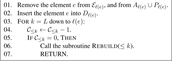
is at level`(s) =b(s)with weightW∗(s) = 0, and hence Invariants3.1,3.2,3.3are vacuously true. Handling the deletion of an element:When an elementegets deleted, we call the subroutine described in Figure1. Steps 01 – 02 in Figure1were explained underCase (a)in Section3.1, whereas steps 03 – 07 in Figure1were explained while defining the countersC≤i.
01. Remove the elementefromE`(e), and fromA`(e)∪P`(e).
02. Insert the elementeintoD`(e). 03. FORk=Ldown to`(e): 04. C≤k← C≤k−1. 05. IFC≤k= 0, THEN
06. Call the subroutine REBUILD(≤k).
07. RETURN.
Figure 1: Handling the deletion of an elemente.
Handling the insertion of an element:When an elementegets inserted, we call the subroutine in Figure2. Steps 02 – 04 and 05 – 09 in Figure2were respectively discussed underCase (b)andCase (c)in Section3.1.
01. Leti= max{`(s) :s∈ S, e∈s}.
02. IFthere is at least one sets∈ S ∩ Stight∗ that containse, THEN
03. `(e)←i.
04. Insert the elementeintoEi and intoPi, with weightw(e)←0. 05. ELSE
06. LetSe= {s∈ S, e∈s}be the collection of all sets that containe. Letλ= min{x:W∗(s) +x=csfor somes∈ Se}.
07. `(e)←i.
[image:12.612.163.449.213.316.2]08. Insert the elementeintoEi and intoPi, with weightw(e)←λ. 09. FORall setss∈ Se:W∗(s)←W∗(s) +w(e).
Figure 2: Handling the insertion of an elemente.
Output of our algorithm: We maintain the collection of tight setsS∗
tight = {s ∈ S : (1 +)−1cs ≤
W∗(s)< cs}. We show in Section4thatStight∗ is a(1 +)f-approximate minimum set cover in(S,E). Correctness of the invariants: Suppose that Invariants 3.1, 3.2, 3.3 hold just before the deletion of an elemente. This is handled by the subroutine in Figure1. It is easy to check that steps 01 – 02 in Figure1
donotlead to a violation of any invariant. This is because the elementegets moved fromA∪P toD, but its weightw(e)remains the same, and it still contributes to the weightsW∗(s)of all the setsscontaininge. Similarly, suppose that Invariants 3.1, 3.2 and3.3 hold just before the insertion of an elemente. We handle this insertion by calling the subroutine in Figure2. Consider two possible cases.
Case (a): Steps 02 – 04 get executed in Figure2. In this case, the elementebecomes passive with weight
[image:12.612.131.485.386.533.2]Case (b): Steps 05 – 09 get executed in Figure2. In this case, all the setss∈ S containingehave weights
W∗(s) < (1 +)−1c
s at the timeegets inserted. LetSe0 = arg mins∈Se{cs−W
∗(s)}. After we assign weightw(e)←λto the elemente, every sets∈ Se0 gets weightW∗(s) =cs, and every other sets∈ Se\ Se0 continues to have weightW∗(s)< cs. The weights of the setss∈ S \ Sedo not change. This ensures that Invariants3.2and3.3continue to hold. Finally, revisiting the proof of Claim3.1, we infer that Invariant3.1
also continues to hold sinceebecomes passive with weightw(e) =λ≤(1 +)−`(e).
To summarize, we conclude that if the subroutine REBUILD(≤ j) has the property that a call to this subroutine never leads to a violation of the invariants, then the invariants continue to hold all the time.
3.4 TheREBUILD(≤k)subroutine
A detailed description of the subroutine appears in AppendixB. Here, we summarize a few key properties of this subroutine that will be heavily used in the analysis of our algorithm. Property 3.4 ensures that Invariants 3.2and3.3 never get violated. Property3.5specifies the time taken to implement a call to the subroutine, and how the counters{C≤i}get updated as a result of this call. Property3.6, on the other hand, explains how the subroutine changes the states and levels of different elements in the hierarchical partition.
Property 3.4. If Invariants3.1,3.2,3.3were satisfied just before a call to the subroutineREBUILD(≤ k) for anyk∈[0, L], then these invariants continue to remain satisfied at the end of that call.
Property 3.5. Consider any level k ∈ [0, L]. The time taken to implement a call to REBUILD(≤ k) is proportional toftimes the number of elements inE≤k∪D≤kin the beginning of the call, plusO(log(Cn)/). Furthermore, at the end of this call, we haveC≤j =· |E≤j|for all levelsj ∈[0, k].
Property 3.6. Consider any levelk∈[0, L]and any call to the subroutineREBUILD(≤k).
(1)The call to REBUILD(≤ k) cleans upall the dead elements at level≤ k. Specifically, this means the following. Consider any elementethat belongs toD≤k just before the call to REBUILD(≤ k). Then that elementedoesnotappear in any of the setsA, P,DorRat the end of the call.
(2)The call to REBUILD(≤ k) converts some of the passive elements at level≤ kto passive elements at levelk+ 1, and the remaining passive elements at level≤ k get converted into active elements at level ≤k+ 1. Specifically, letZdenote the set of elements inP≤k just before the call toREBUILD(≤k). Then during the call toREBUILD(≤k), a subsetZ0 ⊆Zof these elements gets added toPk+1, and the remaining elementse∈Z0\Zget added toA≤k+1.
(3)The call toREBUILD(≤ k) moves up some of the active elements at level≤ kto level k+ 1, and the remaining active elements at level≤ kcontinue to be active at level≤k. In other words, the elements in
A≤knever go out of the setA≤k+1during the call toREBUILD(≤k).
(4) The call to REBUILD(≤ k) does not touch the elements at level≥ k+ 1. In other words, for any
i≥k+ 1, if an elementebelonged toAi,PiorDijust before the call toREBUILD(≤k), then it continues to belong to the same setAi, Pi orDiat the end of the call toREBUILD(≤k).
Corollary 3.7. At the end of any call toREBUILD(≤k), we haveDj =Pj =∅for allj∈[0, k].
Proof. Follows from part (1) and part (2) of Property3.6.
4
Analysis of our dynamic algorithm
does not change significantly in between two successive calls to REBUILD(≤j) at any levelj ∈[0, L]. This
happens because of three main reasons (see Figure1). First, we setC≤k =· |E≤k|for allk∈[0, j]at the end of each call to REBUILD(≤j). Second, we decrement the counterC≤kfor allk∈[j, L]each time some element gets deleted from levelj. Third, we call REBUILD(≤k) wheneverC≤kbecomes equal to0. Notation: Throughout the rest of this section, we use the superscript (t) to denote the status of some set/counter at time-stept. For instance, the symbolD≤j(t) will denote the set of dead elements at level≤jat time-stept, and the symbolC≤j(t)will denote the value of the counterC≤j at time-stept.
Lemma 4.1. Fix any level j ∈ [0, L]and consider any two time-steps t0 < t that satisfy the following properties: (1) A call was made to the subroutineREBUILD(≤k) for somek∈[j, L]just before time-step
t0. (2) No call was made toREBUILD(≤k) for anyk ∈[j, L]during the time-interval[t0, t]. LetM≤j(t0→t)
denote the set of elements that got deleted from level≤jduring the time-interval[t0, t]. Then we have:
M
(t0→t)
≤j +C
(t) ≤j =·
A
(t0)
≤j .
Proof. As the subroutine REBUILD(≤k) was called for somek∈[j, L]just before time-stept0, Property3.5
implies thatC≤j(t0)=· A
(t0)
≤j
. Next, note that during the time-interval[t
0, t], no call is made to the subroutine
REBUILD(≤ k) for anyk ∈ [j, L]. Hence, during this time-interval, the counterC≤j gets decremented by
one iff an element gets deleted from level≤j(see Figure1), and the setM≤j(t0→t)consists precisely of these elements. Thus, we infer that:
M
(t0→t) ≤j
+C
(t) ≤j =C
(t0) ≤j =·
A
(t0) ≤j
.
Corollary 4.2. Consider any levelj∈[1, L]and time-stepst0 < tas defined in Lemma4.1. Then we have:
M
(t0→t) ≤j ≤· A
(t0) ≤j
.
Proof. Note that the subroutine REBUILD(≤ j) gets called wheneverC≤j = 0(see Figure1), and before finishing its execution the subroutine resetsC≤j =· |E≤j|(see Property3.5). Thus, the counterC≤jalways remains nonnegative, and in particular we haveC≤j(t) ≥0. The corollary now follows from Lemma4.1.
Corollary 4.3. Consider any levelj∈[1, L]and time-stepst0 < tas defined in Lemma4.1. Then we have:
D
(t) ≤j ≤· A
(t0) ≤j
.
Proof. Since the subroutine REBUILD(≤k) was called for somek∈ [j, L]just before time-stept0, Corol-lary3.7implies thatD(≤jt0)=∅. We now track how the setD≤j changes during the time-interval(t0, t).
Whenever an elementegets deleted from level≤jduring this time-interval, the elementegets added to both the setsD≤j andM(t
0→t)
≤j . On the other hand, whenever the subroutine REBUILD(≤k) gets called for somek ∈[1, j−1], all the dead elements at level≤kget removed from the hierarchical partition (see part (1) of Property3.6). Sincek < j, such a call to REBUILD(≤k) can potentially remove some elements from the setD≤j, but no element fromM(t
0→t)
≤j gets removed due to the call.
Since no call is made to the subroutine REBUILD(≤k) for anyk∈[j, L]during the time-interval[t0, t],
and since D≤j = ∅ at time-stept0, the preceding discussion implies thatD(≤jt) ⊆ M(t
0→t)
≤j . Thus, from Corollary4.2, we get
D
(t) ≤j ≤ M
(t0→t) ≤j ≤· A
(t0) ≤j
.
Lemma 4.4. Consider any levelj ∈[1, L]and time-stepst0< tas defined in Lemma4.1. Then we have:
A
(t) ≤j
≥(1−)· A
(t0) ≤j
Proof. According to part (3) of Property3.6, a call to REBUILD(≤ k) for somek ∈ [1, j−1]can never
decrease the size of the setA≤j. Since no call was made to REBUILD(≤k) for anyk ∈ [j, L]during the time-interval[t0, t], we conclude that: During the time-interval[t0, t], the setA≤j can decrease in size only via deletion of elements from level≤j. Moreover, the setM≤j(t0→t)contains all these deleted elements. Thus, we infer that: A(≤jt0)\A≤j(t) ⊆M≤j(t0→t). Applying Corollary4.2, we now get:
A
(t0) ≤j \A
(t) ≤j ≤ M
(t0→t) ≤j ≤ · A
(t0) ≤j
. In words, at most anfraction of the elements get deleted from the setA≤jduring the time-interval [t0, t]. Hence, it follows that
A
(t) ≤j
≥(1−)· A
(t0) ≤j
.
Corollary 4.5. We always have|D≤j| ≤2· |A≤j|for every levelj∈[0, L].
Proof. Fix any levelj ∈[0, L]and any time-stept. We will show that the lemma holds for leveljat time-stept. Lett0 < tbe the last time-step beforetwith the following property: a call was made to the subroutine REBUILD(≤k) for somek∈[j, L]just before time-stept0. Thus, during the time-interval[t0, t]no call was made to REBUILD(≤k) for anyk∈[j, L]. Hence, Corollary4.3and Lemma4.4imply that:
D
(t) ≤j ≤· A
(t0)
≤j
= (/(1−))·(1−) A
(t0)
≤j
≤(/(1−))· A
(t) ≤j ≤2·
A
(t) ≤j .
The last inequality holds as long as≤1/2. Thus, we infer that|D≤j| ≤2· |A≤j|at time-stept.
4.1 Bounding the update time of our dynamic algorithm
Data structures:We use the following data structures in our dynamic algorithm.
For each leveli∈[1, L], we maintain the setsEi, Ai, PiandDias doubly linked lists. Each entry in each of these lists also maintains a bidirectional pointer to the corresponding element. Using these pointers, we can determine the state of a given element and insert/delete it in a given list inO(1)time.
For every elemente ∈ E ∪D, we maintain its level`(e)and weightw(e). For every sets ∈ S, we also maintain its level`(s)and weightW∗(s)with respect to the shadow input(S,E∗).
Finally, for every leveli∈[0, L], we maintain the counterC≤i.
Theorem 4.6. Our dynamic algorithm has an amortized update time ofO(flog(Cn)/2).
Proof. Recall that every element belongs to at mostfsets. Hence, ignoring the potential call to REBUILD(≤
k), it takesO(f +L) = O(f + log(1+)(Cn)) = O(f + log(Cn)/) time to implement all the steps in Figure1and Figure2. In other words, the update time of our dynamic algorithm is dominated by the time spent on the calls to REBUILD(≤k). Henceforth, we focus on bounding the time spent on these calls.
Fix anyk∈[0, L]and consider any call to REBUILD(≤k) that is made just after some time-step (say)
t. Lett0 < tbe the last time-step beforetwith the following property: a call was made to REBUILD(≤j) for somej∈[k, L]just before time-stept0. SinceE≤k=A≤k∪P≤k, Corollary3.7states that:
D(≤kt0)=P≤k(t0)=∅, and henceE≤k(t0)=A(≤kt0). (4.1)
REBUILD(≤j) for somej∈ [1, k−1]does not change the set of elements inE≤k. Thus, during the time-interval[t0, t], the only way the setE≤k can increase in size is via insertions of elements at levels≤ k. It follows that:E≤k(t) ⊆ E≤k(t0)∪ I≤k(t0→t). SinceE≤k(t0) =A(≤kt0)according to (4.1), we get:
E≤k(t) ⊆A≤k(t0)∪ I≤k(t0→t) (4.2)
Since a call was made to the subroutine REBUILD(≤ k) just after time-step t, it must be the case that
C≤k(t) = 0. Thus, from Lemma4.1we infer that:
M
(t0→t)
≤k =· A
(t0)
≤k
(4.3)
LetT denote the total “cost” (update time) we pay for calling the subroutine REBUILD(≤k) at time-stept. From (4.2), (4.3) and Property3.5, we get:
T =Of · E
(t) ≤k +f·
D
(t) ≤k
+O(log(Cn)/) =Of· A
(t0) ≤k +f·
I
(t0→t) ≤k
+O(log(Cn)/) (4.4)
After each update, our dynamic algorithm (see Figures1and2) makes at most one call to the REBUILD(≤i)
subroutine, over alli∈[0, L]. Hence, we can safely ignore the termO(log(Cn)/)inT above, as this term gets subsumed within our desired update time bound ofO(flog(Cn)/2). Wesplit-upthe remaining chunk ofT into two parts: T1 = O
f· A
(t0) ≤k
andT2 = O
f· I
(t0→t) ≤k
. Wechargethe cost T1 (resp. T2)
by distributing it evenly among the elements that get deleted from (resp. inserted into) level≤kduring the time-interval[t0, t]. We now bound the total charge accumulated by an element in this fashion.
First, note that as per (4.3),· A
(t0) ≤k
elements get deleted from level≤kduring the time-interval[t 0, t]. When we distribute the costT1evenly among them, each of these elements accumulate a charge ofO(f /).
Now, consider any elementethat accumulates some charge in this fashion due to the call to REBUILD(≤k) just after time-stept. By definition, this elementegets deleted during the time-interval[t0, t]. Accordingly, it is not possible for the same elementeto accumulate a similar charge from the same levelkat some future time-stept00> t.9 To summarize, an elementegets charged at most once from a given level in this manner.
Next, note that when we distribute the costT2evenly among the elements inI(t 0→t)
≤k , each such element accumulates a charge ofO(f). Consider any elementethat accumulates some charge from levelkjust after some time-steptin this manner. By definition, this element got inserted during the time-interval[t0, t], and thus it will never get charged due to a call to REBUILD(≤k) at some future time-stept00> t. To summarize,
here again we derive that an elementegets charged at most once from a given level in this fashion.
From the discussion in the preceding two paragraphs, we conclude that any elementeaccumulates a charge of at mostO(f /+f) =O(f /)from each level. Thus, the total charge accumulated by any element is at mostO((f /)L) =O((f /) log(1+)(Cn)) =O(flog(Cn)/2). This means that the amortized update
time of our dynamic algorithm is alsoO(flog(Cn)/2).
4.2 Bounding the approximation ratio of our dynamic algorithm
Our main result is summarized in the theorem below.
Theorem 4.7. In the hierarchical partition maintained by our dynamic algorithm, the tight sets Stight∗ = {s∈ S : (1 +)−1cs≤W∗(s)≤cs}form a(1 + 5)f-approximate minimum set cover in(S,E).
9
We now give a high-level overview of the proof of the above theorem. First, recall thatE∗ = E ∪D. Hence, the element-weights {w(e)} define a valid fractional packing in the shadow-input (S,E∗) as per Invariant3.2, and the sets inStight∗ form a valid set cover in(S,E∗)as per Invariant3.3. As per Invariant3.3, every elemente∈ E ∪Dis contained in at least one tight set. In other words, the fractional packing{w(e)}
isapproximately maximal, in the sense that every element belongs to at least one set whose weight cannot be increased by more than(1 +)-factor. Armed with this observation, it is not too difficult to show that the size of the dual set cover (defined by the tight sets) is within a multiplicative factor(1 +)f of the size of the fractional packing{w(e)}in(S,E∗). This already implies that the collection of tight setsS∗
tightforms a
(1 +)f-approximate minimum set cover in the shadow input (see Lemma4.9). The key challenge now is to show that the sets inStight∗ also constitute an approximately minimum set cover in the actual input(S,E). To address this challenge, we exploit the fact that the number of elements in D is relatively small compared to the number of elements in A (see Corollary 4.5). This implies that the total weight of the elements inDis also small compared to the total weight of the elements inA(see Lemma4.8). Hence, even if we delete all the elements inDfrom the fractional packing{w(e)}, the objective value of the resulting solution will remain close to the objective value of the original fractional packing, which in turn was within a factor(1+)f of the total cost of the sets inStight∗ . So we expect that the size of the new fractional packing (after deleting the elements inD) will be very close to(1 +)f·c
Stight∗ , wherec
Stight∗ is the total cost of the sets inS∗
tight(see Corollary4.10). Now, this also happens to be a valid fractional packing in the actual input(S,E), because we already hadW∗(s) ≤cs for all setss∈ S and removing the elements inDwill notincrease the weights of the sets any further. On the other hand, the sets inStight∗ form avalidset cover in the actual input(S,E)as well, as Invariant3.3holds for alle∈ E. In other words, we have identified a valid fractional packing and a valid set cover in(S,E)whose objective values are within a(1 +O())f-factor of each other. So the corresponding set cover must be an approximately minimum set cover in(S,E).
Lemma 4.8. We always haveP
e∈Dw(e)≤2· P
e∈Aw(e).
Proof. We first express the weight of an elemente as a sum ofincrements, where each increment corre-sponds to a specific levelk≥`(e). To be more precise, we define:
∆k = (
(1 +)−k fork=L;
(1 +)−k−(1 +)−(k+1) for0≤k < L.
From Invariant3.1, we conclude that:
w(e) = (1 +)−`(e)=
L X
k=`(e)
∆kfor every elemente∈A. (4.5)
w(e) ≤ (1 +)−`(e)=
L X
k=`(e)
∆kfor every elemente∈D. (4.6)
Now, we derive that:
X
e∈D
w(e) ≤ X e∈D
L X
k=`(e) ∆k=
L X
k=0
X
e∈D:`(e)≤k
∆k= L X
k=0
∆k· |D≤k| ≤ L X
k=0
∆k·2|A≤k|
= 2· L X
k=0 X
e∈A:`(e)≤k
∆k= 2· X
e∈A L X
k=`(e)
∆k= 2· X
e∈A
w(e).
Lemma 4.9. We haveP
e∈E∗w(e)≥((1 +)f)
−1·cS∗ tight
.
Proof. By Invariant3.3, every elemente∈ E ∪D=E∗ belongs to at least one set inStight∗ . We sum over the weights of these elements. Sincef is an upper bound on the maximum frequency of an element, we get:
X
e∈E∗
w(e)≥f−1X
s∈S
W∗(s)≥f−1 X
s∈S∗
tight
W∗(s)≥f−1 X
s∈S∗
tight
(1 +)−1cs= ((1 +)f)−1·c Stight∗
.
Corollary 4.10. We haveP
e∈Ew(e)≥((1 +)(1 + 2)f) −1·
c
Stight∗ .
Proof. Using Lemma4.8, we derive that:
1 + (2)−1·X e∈A
w(e) ≥ (2)−1· X e∈D
w(e) +X
e∈A
w(e) !
Multiplying both sides in the above inequality by2(1 + 2)−1 = (1 + (2)−1)−1, we get:
X
e∈A
w(e)≥(1 + 2)−1· X e∈A∪D
w(e). (4.7)
Now, adding the weights of the passive elements – given byP
e∈Pw(e)– on both sides of (4.7), we get: X
e∈A∪P
w(e)≥(1 + 2)−1· X e∈A∪P∪D
w(e). (4.8)
SinceE =A∪P andE∗=A∪P∪D, the corollary follows from (4.8) and Lemma4.9.
Proof of Theorem4.7. By Invariant3.3, every elemente ∈ E belongs to at least one set inStight∗ . In other words, the collection of setsStight∗ forms a valid set cover in the input(S,E). Next, from Invariant3.2we infer the following bound on the weightW(s)of any sets∈ S:
W(s)≤W∗(s)≤csfor all setss∈ S.
The first inequality holds since we consider the weights of the elementse∈ E∗ =E ∪Dwhile calculating
W∗(s), whereas we only consider the weights of the elementse ∈ E while calculating W(s). Thus, the element-weights{w(e)}e∈E form a validfractional packingin(S,E). Finally, Corollary4.10implies that the size of this fractional packing is at leastαtimes of the total cost of the set coverStight∗ in(S,E), where
α= ((1 +)(1 + 2)f)−1≥((1 + 5)f)−1when0< <1/2. Theorem4.7now follows from Lemma2.1.
Acknowledgement
The research leading to these results has received funding from the European Research Council under the European Union’s Seventh Framework Programme (FP/2007-2013) / ERC Grant Agreement no. 340506.
References
[1] Amir Abboud, Raghavendra Addanki, Fabrizio Grandoni, Debmalya Panigrahi, and Barna Saha. Dy-namic set cover: Improved algorithms & lower bounds. InSTOC. ACM, 2019. (cit. on p.1,2,3)
[2] Surender Baswana, Manoj Gupta, and Sandeep Sen. Fully dynamic maximal matching in o(log n) update time (corrected version).SIAM J. Comput., 47(3):617–650, 2018. announced at FOCS’11. (cit. on p.3)
[3] Aaron Bernstein and Shiri Chechik. Deterministic decremental single source shortest paths: beyond the o(mn) bound. InSTOC, pages 389–397. ACM, 2016. (cit. on p.2)
[4] Aaron Bernstein and Shiri Chechik. Deterministic partially dynamic single source shortest paths for sparse graphs. InSODA, pages 453–469. SIAM, 2017. (cit. on p.2)
[5] Sayan Bhattacharya, Deeparnab Chakrabarty, and Monika Henzinger. Deterministic fully dynamic approximate vertex cover and fractional matching in O(1) amortized update time. In IPCO, volume 10328 ofLecture Notes in Computer Science, pages 86–98. Springer, 2017. (cit. on p.1,2,5)
[6] Sayan Bhattacharya, Monika Henzinger, and Giuseppe F. Italiano. Deterministic fully dynamic data structures for vertex cover and matching. SIAM J. Comput., 47(3):859–887, 2018. announced at SODA’15. (cit. on p.2)
[7] Sayan Bhattacharya, Monika Henzinger, and Giuseppe F. Italiano. Dynamic algorithms via the primal-dual method. Inf. Comput., 261(Part):219–239, 2018. announced at ICALP’15. (cit. on p.1,2,3,5)
[8] Sayan Bhattacharya, Monika Henzinger, and Danupon Nanongkai. New deterministic approximation algorithms for fully dynamic matching. InSTOC, pages 398–411. ACM, 2016. (cit. on p.2)
[9] Sayan Bhattacharya, Monika Henzinger, and Danupon Nanongkai. New deterministic approximation algorithms for fully dynamic matching. InSTOC, pages 398–411. ACM, 2016. (cit. on p.2)
[10] Julia Chuzhoy and Sanjeev Khanna. A new algorithm for decremental single-source shortest paths with applications to vertex-capacitated flow and cut problems. InSTOC. ACM, 2019. (cit. on p.2)
[11] Vasek Chv´atal. A greedy heuristic for the set-covering problem. Math. Oper. Res., 4(3):233–235, 1979. (cit. on p.1)
[12] Irit Dinur, Venkatesan Guruswami, Subhash Khot, and Oded Regev. A new multilayered PCP and the hardness of hypergraph vertex cover. SIAM J. Comput., 34(5):1129–1146, 2005. announced at STOC’03. (cit. on p.1)
[13] Irit Dinur and David Steurer. Analytical approach to parallel repetition. In STOC, pages 624–633. ACM, 2014. (cit. on p.1)
[14] Anupam Gupta, Ravishankar Krishnaswamy, Amit Kumar, and Debmalya Panigrahi. Online and dy-namic algorithms for set cover. InSTOC, pages 537–550. ACM, 2017. (cit. on p.1,2,5)
[15] Monika Henzinger, Sebastian Krinninger, and Danupon Nanongkai. Dynamic approximate all-pairs shortest paths: Breaking the o(mn) barrier and derandomization. SIAM J. Comput., 45(3):947–1006, 2016. announced at FOCS’13. (cit. on p.2)
[17] Danupon Nanongkai and Thatchaphol Saranurak. Dynamic spanning forest with worst-case update time: adaptive, las vegas, and o(n1/2 -)-time. InSTOC, pages 1122–1129. ACM, 2017. (cit. on p.2)
[18] Danupon Nanongkai, Thatchaphol Saranurak, and Sorrachai Yingchareonthawornchai. Breaking quadratic time for small vertex connectivity and an approximation scheme. In STOC. ACM, 2019. (cit. on p.2)
[19] Peter Slav´ık. A tight analysis of the greedy algorithm for set cover. J. Algorithms, 25(2):237–254, 1997. (cit. on p.1)
[20] Shay Solomon. Fully dynamic maximal matching in constant update time. In IEEE 57th Annual Symposium on Foundations of Computer Science, FOCS, pages 325–334, 2016. (cit. on p.3)
A
A Static Primal-Dual Algorithm for Minimum Set Cover
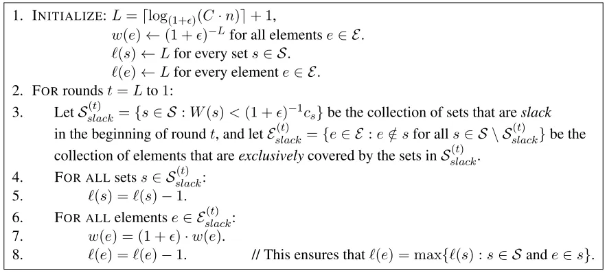
We use the same notations as in Section2. The discretized primal-dual algorithm proceeds inLrounds (see Figure3). In the beginning, we start by assigning a weightw(e) = (1 +)−L≤(Cn)−1to every element
e∈ E, and alevel`(s) =`(e) =Lto every sets∈ Sand every elemente∈ E. Since each set inScontains at mostnelements, at this point in time we haveW(s) = P
e∈sw(e) ≤ n·(Cn)−1 = 1/C for all sets
s∈ S. Hence, from (1.1) we infer that0≤W(s)≤csfor all setss∈ S. In other words, we have a valid fractional packing at this point in time. Throughout the rest of this section, we say that a sets∈ S istight if(1 +)−1cs≤W(s)≤cs, andslackif0≤W(s)<(1 +)−1cs.
In the beginning, we start with a countert=L. The value oftkeeps decreasing by one until we reach
t = 0. Each value of t corresponds to a distinct round in the algorithm. In each round t, we increase (by a (1 +) factor) the weights of the elements that are exclusively covered by the slack sets, and we decrease by one the levels of the concerned sets (that were slack in the beginning of the current round) and elements (whose weights got increased in the current round). Thus, there areLrounds overall, one for each
t∈ {L, . . . ,1}. At the end of round1, we have ahierarchical partitionofSintoL+ 1levels{L, . . . ,0}. We now describe a few key properties that are satisfied at the end of the algorithm in Figure3.
1. INITIALIZE:L=dlog(1+)(C·n)e+ 1,
w(e)←(1 +)−Lfor all elementse∈ E.
`(s)←Lfor every sets∈ S.
`(e)←Lfor every elemente∈ E. 2. FORroundst=Lto1:
3. LetSslack(t) ={s∈ S :W(s)<(1 +)−1c
s}be the collection of sets that areslack in the beginning of roundt, and letEslack(t) ={e∈ E :e /∈sfor alls∈ S \ Sslack(t) }be the collection of elements that areexclusivelycovered by the sets inSslack(t) .
4. FOR ALLsetss∈ Sslack(t) : 5. `(s) =`(s)−1.
6. FOR ALLelementse∈ Eslack(t) : 7. w(e) = (1 +)·w(e).
[image:20.612.85.527.468.667.2]8. `(e) =`(e)−1. // This ensures that`(e) = max{`(s) :s∈ S ande∈s}.
Figure 3: A static(1 +)f-approximation algorithm for minimum set cover.
Proof. (Sketch) Fix any elemente ∈ E. Initially, every set and every element is assigned to levelL. See step 1 in Figure3. At this point, we clearly have`(e) = max{`(s) : s∈ S, e∈ s}. Subsequently, during a given roundt, we decrement the level ofeonly ife ∈ Eslack(t) . See step 8 in Figure 3. Now, note that if
e ∈ Eslack(t) , then by definition every set s ∈ S containingebelongs toSslack(t) . Furthermore, as is evident from step 5 in Figure3, during roundtwe also decrement the level of every sets∈ Sslack(t) . Thus, we always have:`(e) = max{`(s) :s∈ S, e∈s}.
Next, note that as per step 1 in Figure3, we initially have`(e) =Landw(e) = (1+)−L= (1+)−`(e). Subsequently, whenever we increasew(e)by a factor of(1 +), we also decrement the level`(e)by one (see steps 7, 8 in Figure3). Hence, it follows thatw(e) = (1 +)−`(e)at the end of the algorithm.
Claim A.2. For every elemente∈ E, at least one of the sets containingelies at level≥1(i.e.,`(e)≥1). Proof. (Sketch) Fix any elemente∈ E. For the sake of contradiction, suppose that`(e) = 0at the end of the algorithm. This implies thate∈ Eslack(1) in the beginning of round1. This is because only the elements inEslack(1) get moved down to level0. Hence, as per the proof of ClaimA.1, we havew(e) = (1 +)−1 in the beginning of round1. This means that every sets ∈ Scontaining the element ehasW(s) ≥ w(e) ≥ (1 +)−1 ≥ (1 +)−1cs in the beginning of round1. The last inequality holds since cs ≤ 1for all sets
s∈ S, as per (1.1). Accordingly, no set containingecan be part ofSslack(1) . This leads to a contradiction, for we assumed thate∈ Eslack(1) , which in turn means thateis exclusively covered by the sets fromSslack(1) .
Corollary A.1. We haveEslack(1) =∅.
Proof. Follows from the proof of ClaimA.2.
Claim A.3. For every sets∈ S we have:
W(s)∈ (
[(1 +)−1c
s, cs] if`(s)>0;
[0,(1 +)−1cs) else if`(s) = 0.
Proof. (Sketch) Fix any sets∈ S. Initially, in the beginning of roundL, we haveW(s) =P
e∈sw(e) ≤ |E| ·(Cn)−1 = 1/C. From (1.1), we conclude that0 ≤W(s) ≤csat this point in time. Subsequently, in each roundt∈ {L, . . . ,1}, we keep moving down the setsto levelt−1iff we haveW(s)<(1 +)−1csin the beginning of the current round. Consider such a roundtwhere the setsgets moved down to levelt−1. In the beginning of roundt, we hadW(s) <(1 +)−1cs. During roundt, we only increase (by a(1 +) factor) the weightsw(e)of some of the elementsecontained ins. Thus, even at the end of roundt, we have
W(s)≤cs. This is sufficient for us to conclude that at the end of the algorithm, we have:
(a)Ws≤csand (b)Ws∈[(1 +)−1cs, cs]if`(s)>0.
It remains now to consider the case where`(s) = 0at the end of the algorithm. If this is the case, then we must have hads∈ Sslack(1) , for only the sets inSslack(1) gets demoted to level0during round1. Accordingly, we infer thatWs <(1 +)−1csin the beginning of round1. Now, by CorollaryA.1, we haveEslack(1) =∅. In other words, no element changes its weight during round1. So the weightW(s)of the setsalso remains unchanged during round1. We accordingly infer thatW(s)<(1 +)−1csat the end of the algorithm.
Claim A.4. Consider any sets∈ S. At the end of the algorithm in Figure3, it must be the case that every elemente∈sis at a level`(e)≥b(s).
A.1 Post-processing
We now need to slightly modiy the hierarchical partition returned by the algorithm in Figure3. Specifically, armed with ClaimA.4, we perform the following post-processing step:
• We move every sets∈ Sat level`(s)< b(s)to its base levelb(s).
Consider any sets ∈ S that changes its level due to the post-processing step described above. ClaimA.4
implies that moving the setsup to levelb(s) does not affect the level (and weight) of any elemente. In other words, the post-processing step does not change any of the weights{W(s)}and{w(e)}.
After this post-processing, the resulting hierarchical partition satisfies the three crucial properties stated towards the end of Section2. Property2.2follows from ClaimA.1, Property 2.3follows from ClaimA.3
and the fact thatb(s)≥0for all setss∈ S, and Property2.4follows from ClaimA.2and ClaimA.3.
B
A detailed description of the
R
EBUILD(
≤
k
)
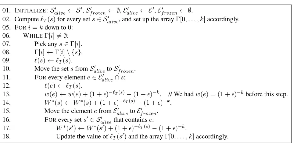
subroutine
The subroutine works in 9 steps. We explain them in details below.
Step 1:Scan through all the elements inE≤k∪D≤kand identify the collection of setsS0 ={s∈ S :`(s)≤
k, s∩(E≤k∪D≤k) 6= ∅}. A set belongs toS0iff it is at level≤ kand contains at least one element from E≤k∪D≤k. These are the sets whose levels and weights will be affected due to the call to REBUILD(≤k).
Remark:Consider any elemente∈ E≤k∪D≤k. These are the elements that get affected due to the call to REBUILD(≤k). Since`(e) = max{`(s) : s∈ S, e∈s} ≤k, it follows that every sets∈ S containinge
lies at a level`(s)≤k. In other words, every sets∈ Sthat contains such an elementealso belongs to the collectionS0. We will be using this observation throughout the rest of this section.
Step 2: Remove all the elements fromD≤k, and accordingly modify the weightsW∗(s)of the concerned sets inS0. At the end of this step, we haveD≤k=∅. This is stated in part (1) of Property3.6.
Step 3: For every elemente∈A≤k, setw(e) ←(1 +)−(k+1)and accordingly modify the weightW∗(s) of each sets∈ S0 that containse. Next, for every elemente∈P≤k, setw(e)←0, and accordingly modify the weightW∗(s)of each sets∈ S0that containse.
Remark:Steps 2 and 3 can only decrease the weightsW∗(s)of the setss∈ S0. This is because just before step 2 we hadw(e)≥(1 +)−kfor all elementse∈A≤k, andw(e)≥0for all elementse∈P≤k. We also hadW∗(s)≤csfor all setss∈ S0, as per Invariant3.2. Now, Step2removed the elements fromD≤kand Step3decreased the weights of the elements inA≤k∪P≤k. Thus, we continue to haveW∗(s)≤csfor all setss∈ S0 even after Step 3.
Step 4:FORevery elemente∈P≤k:
• LetS0
e⊆ S0 denote the collection of all sets that containe. Note that|Se0| ≤f. • (a) IFW∗(s)≤cs−(1 +)−(k+1)for all setss∈ Se0, THEN
– Increase the weight of elementefrom0(see Step 3 above) tow(e)←(1 +)−(k+1), move the elementefromP≤ktoA≤k, and accordingly modify the weightW∗(s)of every sets∈ Se0.
• (b) ELSE
– Letλ= min{x:W∗(s) +x=csfor somes∈ Se0}. Note that in this caseλ <(1 +)−(k+1). – Increase the weight of elementefrom0(see Step 3 above) tow(e) ← max(0, λ), and