Image Reconstruction via Manifold Constrained
Convolutional Sparse Coding for Image Sets
Linlin Yang
1∗, Ce Li
2∗, Jungong Han
3, Qixiang Ye
4, Chen Chen
5, Xianbin Cao
6, Baochang Zhang
1†,
Wanquan Liu
7Abstract—Convolution sparse coding (CSC) has attracted much attention recently due to its advantages in image reconstruction and enhancement. However, the coding process suffers from perturbations caused by variations of input samples, as the consistence of features from similar input samples are not well addressed in the existing literature. In this paper, we will tackle this feature consistence problem from a set of samples via a proposed manifold constrained convolutional sparse coding (MCSC) method. The core idea of MCSC is to use the intrinsic manifold (Laplacian) structure of the input data to regularize the traditional CSC such that the consistence between features extracted from input samples can be well preserved. To implement the proposed MCSC method efficiently, the alternating direction method of multipliers (ADMM) approach is employed, which can consistently integrate the underlying Laplacian constraints during the optimization process. With this regularized data structure constraint, the MCSC can achieve a much better solution which is robust to the variance of the input samples against over-complete filters. We demonstrate the capacity of MCSC by providing the state-of-the-art results when applied it to the task of reconstructing light fields. Finally, we show that the proposed MCSC is a generic approach as it also achieves better results than the state-of-the-art approaches based on convolutional sparse coding in other image reconstruction tasks, such as face reconstruction, digit reconstruction and image restoration.
Index Terms—Light Field, Image Reconstruction, Image Deblurring, Convolutional Sparse Coding, Manifold Constrained Convolutional Sparse Coding.
F
1
I
NTRODUCTIONW
ITH the increasing number of images and videosproduced in our everyday life, batch data processing techniques which can deal with high-volume data contain-ing significant illumination variation, blurrcontain-ing, and severe noise, are highly demanded. For instance, high-resolution light field imaging is a typical batch system applied on a set of images captured from large camera arrays or a
hand-held camera moved over time around the scene [1], [2]. To
handle the challenging problem caused by high sampling rate and huge-volume samples captured in various of ex-ternal conditions (i.e., lighting variations), different kinds of techniques that can reconstruct dense light fields from fewer samples are developed based on various prior assumptions
made about the data [2]. When processing batch images,
researchers reach a consensus that the data structure as a common prior should be given much attention, which has been evidenced first in visualizing high-dimensional data in
the low-dimension space [3], [4], and then some successful
applications in the learning paradigm [5], [6], [7]. Especially,
the data structure embedded into a constraint model could be used to simplify the learning process while improving
• Linlin Yang and Ce Li have equal contribution to the paper. • 1. Department of Automation, Beihang University, Beijing, China.
E-mail: [email protected]; correspondence.
• 2. China University of Mining & Technology, Beijing, China.
• 3. School of Computing & Communications, Lancaster University, LA1 4YW, UK.
• 4. University of Chinese Academy of Sciences, Beijing, China. • 5. University of Central Florida, Orlando, FL, USA.
• 6. School of Electronic and Information Engineering, Beihang University • 7. Curtin University, Perth, Australia.
Manuscript received December 30, 2016.
Coding
Reconstruction
Dictionary
CSC
Input
Input Reconstruction
Dictionary
Coding MCSC
[image:1.612.325.545.375.547.2]Ï
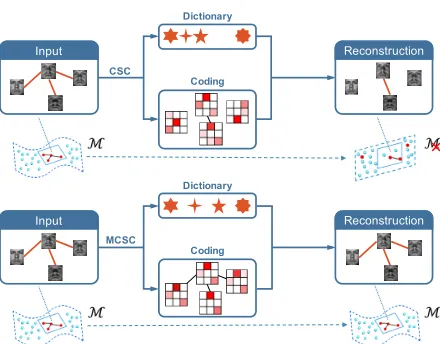
Fig. 1. Illustration of CSC and MCSC for image reconstruction. Re-constructed images by CSC that lacks structure constraint suffer from the perturbation caused by the noised or corrupted input samples. In contrast, the reconstructed images by MCSC with manifold constraint is more consistent with the input data structure. As a property of MCSC, the manifold structure of input data is preserved, leading to more rea-sonable reconstruction results.
the solution quality by the regularization technique, e.g.,
manifold regularization [5], which can be found in the latest
learning algorithms [6], [7]. As detailed in [7], the constraints
JOURNAL OF SELECTED TOPICS IN SIGNAL PROCESSING 2
In this paper, we revisit the convolution sparse coding
(CSC) [8] by considering the data on a Laplacian manifold.
The CSC or deconvolution, as one of fundamental tools in machine learning, has been demonstrated to have important applications in a broad range of computer vision problems including feature learning, particularly related to the
pre-training of the CNN filters [9], image deionising and/or
reconstruction [9], [10], [11], [12] , super-resolution [13],
trajectory reconstruction [14], automatic music transcription
[15] and neuronal ensemble identification [16]. The
conven-tional CSC method was improved by new coding or
dictio-nary learning approaches in theory [17], [18], [19]. Based
on the convolution operator and sparse coding, the CSC reconstructs the vectorized input images with vectorized sparse feature maps and convolutional kernels. There are some works addressing the deficiency of the CSC based on an alternating direction method of multipliers (ADMM)
approach with the mixing matrix [8]. In [20], the extended
CSC has been proposed by considering local features depen-dency for image reconstruction as a potential direction of CSC, but the authors there only sketched out the idea with neither implementation details nor sufficient experimental results. Nevertheless, the data structure of input samples is not fully utilized in the existing CSC methods and the consistence of the features for similar input samples cannot be guaranteed. In other words, the coding results for similar input samples may vary dramatically because the neighbor-hood information in the data-set is ignored. With the over-complete filter set, the coding process without consistence constraints would suffer from the perturbations caused by the variations of input samples as they might be distorted
or corrupted. As shown in Fig.1, the neighborhood of
input images in the reconstruction task is emphasized via a manifold structure constraint.
In this paper, we will consider the mutual dependence among observations, which would result in large variations in the reconstructed data once it is ignored and then this provides some new insights on the CSC with manifold constraints. In particular we have an intuition on the data-set structure that was neglected: the data lying on a spe-cific manifold can be used to improve solutions for some applications. For such purpose, we propose a new scheme
of the CSC as shown in Fig.1 for image reconstruction.
Being different from the traditional CSC without structure constraint, the coding process of the proposed manifold constrained convolutional sparse coding (MCSC) is imposed to be consistent with the data structure, while the learning algorithm is implemented with the regularization technique to solve the ill-posed problem. As an important property of the MCSC, the manifold structure can be preserved, whilst leading to a better reconstruction than the conventional CSC. Furthermore, based on recent advantages in ADMM, we can efficiently solve the proposed MCSC problem based on a new manifold constraint model. One should notice that there exist some previous works to incorporate the manifold
structure into deep learning [7] or sparse coding [6], [21].
However, to the best of our knowledge, this is the first time that manifold constraint is introduced for the CSC. In summary, we have the following contributions in this paper.
1. The manifold structure considered as a constraint is
embedded into the CSC and the proposed problem is theoretically investigated, by which the consistence of features for similar input samples can be preserved. Con-sequently, the reconstruction performance is improved as the implicit manifold structure is preserved.
2. The derived theoretical results show that imposing Lapla-cian manifold constraint on the input data is equivalent to imposing regularization terms on the coding and dictionary, which provides an insight for other similar
methods [6], [21].
3. Extensive experimental results on image reconstruction, image de-blurring and light field reconstruction show a consistent improvement of performance with respect to the existing state-of-the-art algorithms based on CSC.
The rest of the paper is organized as follows. Section 2
introduces the related works, and Section 3 describes the
details of the proposed method. Experiments and results are
presented in Section4, and Section5concludes the paper.
2
R
ELATEDW
ORKDifferent from existing sparse coding algorithms for classi-fication, the reconstruction and coding tasks that assume independent observations during the learning procedure, the conventional CSC explicitly models local interactions through the convolution operator, and the resulting opti-mization is considerably more complicated than traditional sparse coding, especially in light field reconstruction.
In [9], [10], [11], [12], some hierarchical models that learn
image decompositions via the CSC are proposed in feature learning. Moreover, an efficient feed-forward encoder that can predict sparse features was proposed for classification,
which is particularly used to train the CNN filters [9],
[22]. With the guarantee that neural activity is sparse in
both space and time, Andilla et al.[16] proposed a sparse
deconvolution approach in both space and time domain for
calcium image sequences. Serranoet al.[23] verified the CSC
on the high-speed video analysis task. The CSC also has attracted growing attention in processing different
recon-struction tasks. Wohlberget al.[17] proposed an extended
CSC algorithm by using an augmented dictionary to
incor-porate the impulse noise images. Heideet al. [8] proposed
a splitting-based ADMM approach with the mixing matrix
to process the incomplete images and Serrano et al. [18]
proposed a variant of CSC to recover high dynamic range images (HDRI), which achieved superior performances. In addition to the applications mentioned above, the CSC
also has been utilized in super-resolution [13], trajectory
reconstruction [14], automatic music transcription [15] and
neuronal ensemble identification [16]. Meanwhile, based
on recent advances in optimization [24], [25], varieties of
efficient approaches to solve the CSC problems have been
proposed, such as, the frequency domain method [26] and
the splitting-based ADMM approach [8].
Recently, researchers have started to explore compres-sive light field acquisition with a single camera. The optical
coding strategies include coded apertures [27], [28], coded
lenslets [27], and a combination of coded mask and aperture
[29].The conventional methods require multiple images to
of shots compared to their non-compressive counterparts.
Marwah et al. [1] used sparse coding techniques to learn
a dictionary of basis vectors for representing light fields, in which the dictionary is chosen so that training light fields may be represented as sparse vectors. The underly-ing assumption is that new light fields will have similar
structure to those in their training data. Similarly, Shiet al.
[2] proposed the continuous sparse structure in the Fourier
domain for light field reconstruction.
Different from the existing works, we present here a new method that exploits Laplacian structure as constraints in the ADMM framework, in which we emphasize on the dependence among samples into the CSC. As a theoretical contribution, we show that the Laplacian manifold structure from data samples can be considered as regularization terms imposed on coding coefficients and dictionary. This makes
our work significantly different from [21], where the
Lapla-cian regularization on coding coefficients is used only for sparse coding. Instead, we focus on the convolution sparse coding with Laplacian regularization on both coding and dictionary learning in the ADMM framework. Our method
is also different from [20], which is based on an assumption
that Laplacian regularization is imposed on only a single image, whereas we focus on a batch of images.
3
M
ANIFOLDC
ONSTRAINEDCSC
In this section, we present how manifold can be incorpo-rated into the CSC as a constraint and then construct the MCSC. We then solve the MCSC problem in the ADMM framework with theoretical analysis.
3.1 Laplacian Manifold for the CSC
As one of increasingly important tools in machine learning and computer vision, the CSC method can be used to learn the features subsequently used for classification and reconstruction tasks. Based on the convolution operator and sparse coding, the CSC is formulated as:
minimize d,z
1 2
N
X
n=1
yn−
K
X
k=1
dk∗znk
2
2
+β
N
X
n=1
K
X
k=1
kznkk1
subject to kdkk
2
2≤1 ∀k∈ {1, . . . , K},
(P1)
where yn ∈ RL1 are vectorized input images, zn
k ∈ R L1
are vectorized sparse feature maps and dk ∈ RL2 are the
vectorized convolutional kernels.N is the number of input
images, β is the sparsity parameter, K is the number of
the kernels and ∗ is the 2D convolution operator defined
on the vectorized inputs. The formulation (P1) can be gen-erally customized for different applications. In the above
formulation, it is assumed thatyn ∈RL1 are independent.
We assume that the input samples yn ∈ RL1 are lying
on a manifold. To utilize the data structure prior, we first reformulate (P1) as:
minimize d,z
1
2ky−Hvk
2
F+β N
X
n=1
K
X
k=1
(kznkk1+1
2kz
n kk
2 2)
subject to kdkk
2
2≤1 ∀k∈ {1, . . . , K}
vn∈ M,
(P2)
where vn = PK
k=1dk ∗ znk, v = [v
1, . . . ,vN], y =
[y1, . . . ,yN]. Mis a set of samples representing the
un-derlying manifold. To encourage a grouping effect, where strongly correlated filters tend to be in or out of the model
together, we choose elastic net constraints [30] instead of
sparsity constraints.His a diagonal matrix whose diagonal
entries are either 1 or 0, keeping or killing the corresponding pixels for image reconstruction, or a measurement matrix containing the sheared mask code of multiple recorded sensors for light filed, or a blur matrix given by point spread function (PSF) and boundary condition for de-blurring, which allows us to gain the robustness in the CSC frame-work for the complex situations, such as motion blur, out-of-focus blur and illumination variation. As a basic intuition,
the manifold structure contained in the data setyn ∈ RL1
should be remained in the convolutional coding process. In
particularyn ∈ Mare the observations of degraded images,
and vn ∈ M are the reconstructions of yn that are thus
subject to a manifold constraint. Again we expect the depen-dence among samples would help us obtain better coding results as well as better solution for the filter learning.
It should be noted that the manifold structure in the original input data is usually not accurate due to the fact that the input data may suffer from noise or corruption. In comparison, we expect the manifold structure becomes
more accurate based on v as a better reconstruction after
removing noise or corruption. Moreover, we prove that the
manifold constraints in terms of v can be interpreted to
be the meaningful regularizations in ADMM, which can improve the kernels’ orthogonally and features’ neighbor relationship. The proof details are presented in Section 3.3.
In order to solve (P2) with structure preservation,vn ∈
M is the only unsolved part. We use the manifold in a
constrained model that is different from the most popular
approaches such as the Local Linear Embedding (LLE) [3]
and the Laplacian with a focus on the data structure
visual-ization. In contrast, the Laplacian Eigenmap [4] provides a
computationally efficient approach to nonlinear dimension-ality reduction that has locdimension-ality-preserving properties with a natural connection to clustering. Here, we calculate the
Laplacian structure ofyin the input space that can be
trans-ferred tovvia a specific constraint function. Technically, the
Laplacian matrixL[4] is used to replacevn ∈ Min P2 and
thus we can obtain the following MCSC formulation.
minimize d,z
1
2ky−Hvk
2
F+
γ
2tr(vLv
T)
+β
N
X
n=1
K
X
k=1
(kznkk1+1
2kz
n kk
2 2)
subject to kdkk
2
2≤1 ∀k∈ {1, . . . , K},
(1)
where L is a Laplacian matrix with a parameterγ, which
weights the contribution of the regularization term. The
solution to Eq.1 with a new manifold constraint function
γ
2tr(vLv
T)
will be investigated based on the ADMM frame-work in the next subsection. It is actually the only part
where manifold plays a role in (P2). According to [5], the
JOURNAL OF SELECTED TOPICS IN SIGNAL PROCESSING 4 3.2 Solution to (P2) Based on the ADMM
The main optimization tool we use in solving this convex
problem Eq.1is ADMM, which is a variant of the standard
Augmented Lagrangian Multiplier (ALM) method that uses partial updates (similar to the Gauss-Seidel method for solving linear equations). The ADMM recently has received much more attention because of its adaptability to several
problems [24]. By iteratively solving a set of simple convex
optimization sub-problems, one can obtain the final solution
of (P2). More details about ADMM can be found in [8], [24],
[25], [31]. The ADMM can solve the sub-convex problems
for two or more variables when one treats one variable each time while other variables are fixed. By exploiting the merits of the ADMM, we develop three update steps as described below: coding update, dictionary update and structure update. The coding update aims for more precise reconstruction coefficients, dictionary update for better rep-resentation and structure update for data manifold structure constraint.
First, the coding update is achieved by:
minimize z
1
2ky−Hvk
2
F+
γ
2tr(vLv
T
)
+β
N
X
n=1
K
X
k=1
(kznkk1+1
2kz
n kk
2 2),
(2)
wherevn =Dzn
,D= [D1, . . . ,DK]is a concatenation of
Toeplitz matrix representing a convolution with the
respec-tive filterdk,z= [z1, . . . ,zN],zn= [znT1 , . . . ,znTk ]
T
.
Next, the dictionary update problem is defined as:
minimize d
1
2ky−Hvk
2
F+
γ
2tr(vLv
T)
subject to kdkk
2
2≤1 ∀k∈ {1, . . . , K},
(3)
wherevn=Znd
,Zn
is a concatenation of Toeplitz matrices
for the respective sparse codesznk,Z= [Z1, . . . ,ZN],d=
[dT
1, . . . ,dTK]T.
And finally, the structure update is shown as:
L= (1−η)L+ηLE(Dz), (4)
where L is initialized equal to LE(y), and LE(·) means
normalized Laplacian matrix function defined in [4] andη
represents update ratio.
To simplify our ADMM, we define four functions that are used to reformulate three mentioned update steps:
f1(x) =
1
2ky−Hxk
2
2, f2(x) =
γ
2tr(xLx
T),
f3(x) =β(kxk1+
1
2kxk
2
2), f4(x) =indc(x),
(5)
where indc(·) represents the indicator function and C =
{x| kSxk22 ≤ 1} . The proximal operators [25] used to
approximate the above four objectives can be derived as
proxλf1(x) = (I+λH
TH)−1(x+λHTy)
proxλf2(x) =x(γλL+I)
−1
proxλf3(x) = (
1
1 +λ)(max(1−
λ
|x|,0)x)
proxλf4(x) =
Sx
kSxk22 kSxk
2 2≥1
Sx else
.
(6)
In Alg.1, we show the iterative steps of the MCSC which
can solve P2 efficiently.
Algorithm 1 - ADMM for (P2)
1: Input image setyand parameters
2: Pre-computeL=LE(y),H
3: Initialized,zrandomly
4: repeat
5: Coding update
z=argmin
z
f1(Dz) +f2(Dz) +
N
X
n=1
K
X
k=1
f3(znk)
6: Dictionary update
d=argmin
d
f1(Zd) +f2(Zd) +
K
X
k=1
f4(dk)
7: Structure update
L= (1−η)L+ηLE(Dz)
8: untilThe maximum number of iteration 50
3.3 Theoretic Analysis of the MCSC
In this subsection, we conduct theoretical analysis for the proposed MCSC in two theorems. In detail, Theorem 1 states
that the Laplacian structure in input data v can
approxi-mately constrain the solution as that in feature spacez
(min-imizingtr(vLvT)is approximated as tr(zLzT)). Theorem
2 proves that in the dictionary update step the Laplacian structure constraint in input data is in fact equal to the
constraint imposed on the dictionary (l2-norm). We describe
two lemmas [32] and then prove our main theorems. The
proofs of lemmas and theorems are shown in the Appendix.
Theorem 1: Given D, and a positive constant α0, we have:
c1tr(zLzT)≤tr(vLvT) +α0
N
X
n=1
K
X
k=1
kznkk22
≤c2tr(zLzT) +α0
N
X
n=1
K
X
k=1
kznkk22,
wherec1andc2are both positive constants.
We observe in this theorem that as a property of the
MCSC, minimizingtr(vLvT)is approximated by
minimiz-ing tr(zLzT). In other words the constraint on the data
v can be transferred to the feature space z. As mentioned
above the Laplacian structure in the input data can constrain the solution as that in the feature space.
Theorem 2:GivenZ, and two positive constantsα0, β0,
we have:
c3kdk22≤tr(vLvT) + (α0+β0)kdk22≤c4kdk22,
wherec3andc4 are both positive constants. Similar to the
observation in Theorem 1, minimizingtr(vLvT)is
approx-imated by minimizingl2-norm ofd. Again the constraint is
transferred from one variable to another.
regularization terms on optimized variables, coding coeffi-cients or dictionary. Comparatively the nonlinear structure constraints in previous works are added on coding
coef-ficients in a brute-force way [6], [21]. As another obvious
advantage of MCSC, the manifold constraint on the data can be more explicitly represented by the optimized variables.
4
E
XPERIMENTSIn this section, we use publicly available datasets to val-idate the effectiveness of the proposed approach on the reconstruction or restoration problems. The experiments are
conducted on face (Yale B) [33], digits (USPS) [34], a
real-application video for car [35], and the Chess [36]. The Yale
B dataset consists of 2,414 frontal-face images from 38
individuals (about 64 images per subject) captured under
various laboratory-controlled lighting conditions. The USPS
dataset is an image dataset including7291training images
and 2007 test images. The video for car consists of 900
97×79-sized images. The Chess [36] database consists of a
17×17grid of viewpoints with1400×800image resolution,
taken from the Stanford light field archive. The comparative methods are some state-of-the-art methods including patch
based sparse coding (PSC) [1], [37], CSC [8], GSR [38] and
MCSCf (see definition in section 4.2). Following the
exper-iments in [8], [37], one part of data is used for training the
dictionary and the other is for testing in reconstruction tasks. To make manifold structure of the data more transparent, we first preprocessed the input images as follows:
Scheme1. Translating one and two pixels in each of the four directions, and rotating the images by one to three degrees.
Scheme2. Random subsampling of the data.
Scheme3. Adding motion blur with 0 mean and 0.01 devi-ations.
To evaluate the quality of the reconstructed images, the signal-to-noise ratio (PSNR, unit:dB) is calculated. The higher PSNR is, the better visual quality is achieved for the reconstructed image. In our experiments, one part of data is used for training the dictionary and the other data is for testing in the reconstruction task. Three parameters
are involved in the MCSC: the sparsity of coding β, the
weight of manifold constraintγand the manifold structure
update ratio η. It should be noted that the parameters are
set according to different applications which might be very different, aiming to deliver a good tradeoff between sparsity and data fit. Regarding to the computational cost, the MCSC can be solved as efficiently as that of the baseline algorithm
[8]. For example, the running time for digit ’0’ in USPS are
respectively 100 minutes and 96 minutes for the MCSC and CSC, on a PC with Intel i7 CPU and 16G RAM.
4.1 Light Field Reconstruction
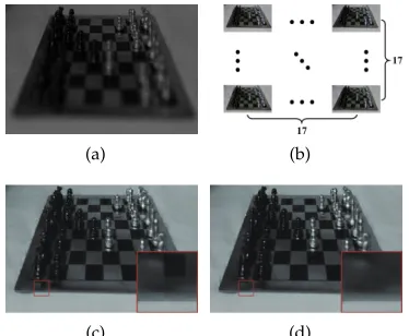
We demonstrate an application of batch light field
recon-struction on the widely used Chess database [36] for MCSC.
The coded 2D projection and the reconstructed light fields
are shown in Fig.2. MCSC allows for higher-resolution
light fields to be reconstructed than previously possible
from a single image, where y is the vectorized observed
sensor image, v is the vectorized light field, and H is a
sparse measurement matrix containing the sheared coded
projection operator on its diagonal, similar to [1]. In this
case, there are17×17angular light field views stacked in
v, the Laplacian matrix is initialized to a suitable default value and the resolution of sensor images are resized into
150×100in our experiment. The recorded sensor image is
stacked iny, and the corresponding measurement matrices
are coded using random masks and stacked in H. The
interesting case of 4D light field reconstruction is addressed to validate the performance of MCSC, in comparison with
the PSC [1] and CSC [8]. Following the baseline methods [1],
[8], we train 648×8-sized filters, and then we setβ = 0.3
in PSC and CSC, whileβ = 0.01,γ = 0.1 and η = 0.01
in MCSC. The results are shown in Fig.2 and Table1. It
can be observed that MCSC achieves better reconstruction
quality (i.e., left-bottom of the chess board) than that of
CSC, based on a compact dictionary due to the regularized manifold structure. The image can be well covered even under complex lighting conditions, occlusion and blurring.
(a) (b)
(c) (d)
Fig. 2. (a) Coded 2D Projection; (b) Reconstructed 4D Light Field; (c) The reconstructed light field by CSC; (d) The reconstructed light field by MCSC.
TABLE 1
Average PSNR (db) for Chess and YaleB01 database.
Method PSC CSC MCSCf MCSC
Chess 29.79 30.96 - 31.54
YaleB01 27.78 28.19 28.40 28.46
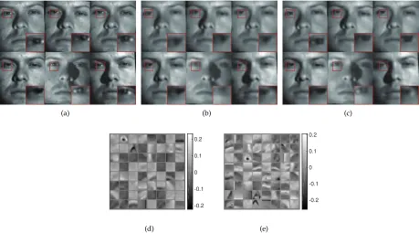
4.2 Face Reconstruction
In this subsection, we evaluate the quality of face image reconstruction in terms of the average PSNR measure using
the extended Yale Face Database B [33]. We process the
images with scheme 1. The images are first resized to 96×84
and then normalized by dividing 255. We trained 6415×15
-sized filters, and compare these MCSC filters with the PSC
[37] and CSC [8]. Besides, we also compare MCSC with
the MCSCf filter. Specifically, MCSCf is defined as the CSC with the manifold constraint on the feature while MCSC is the CSC with the manifold constraint on both data and
feature. We setβ= 0.3in the PSC and CSC, whileβ = 0.3,
γ = 0.1 and η = 0 in MCSCf and MCSC. Six of the
reconstructions and the dictionaries are shown in Fig.3.
[image:5.612.346.533.279.433.2]JOURNAL OF SELECTED TOPICS IN SIGNAL PROCESSING 6
(a) (b) (c)
-0.2 -0.1 0 0.1 0.2
(d)
-0.2 -0.1 0 0.1 0.2
(e)
Fig. 3. (a) Original YaleB01 images; (b) Reconstruction by CSC; (c) Reconstruction by MCSC; (d) CSC dictionary; (e) MCSC dictionary.
TABLE 2
Average PSNR for different digit datasets with 25 7×7-sized filters.
Digit 0 1 2 3 4
PSC 21.00 24.58 23.30 22.83 24.68 CSC 22.65 27.33 24.54 24.66 26.04 MCSCf 23.00 28.10 24.66 25.15 26.42
MCSC 23.14 28.50 24.66 25.20 26.42
Digit 5 6 7 8 9
PSC 23.17 23.28 24.29 23.33 24.27 CSC 24.56 24.79 25.59 24.87 26.08 MCSCf 24.74 25.06 26.14 24.99 26.35
MCSC 24.95 25.23 26.40 25.14 26.42
different reconstruction methods, respectively. All left eyes (upper left) are amplified and compared in the bottom right corner. It can be observed that MCSC achieves much better
visual quality (i.e., eyes) than that of CSC, because of the
compactness of dictionary (Fig.11) that contributes to better
reconstruction results. In terms of the average PSNR values
in Table 1, MCSCf and MCSC improve CSC by 0.21dB
and 0.27dB respectively. It is also obvious that the MCSC achieves a higher performance than other methods.
4.3 Digit Reconstruction
We perform handwritten digit reconstruction on the widely
used the USPS database [34]. We experimented on digit ’0’
to ’9’ respectively with locally contrast normalization [8].
We adopt the parameters in [8] and set β = 1in the PSC
and CSC, while β = 0.8, γ = 0.4, η = 0 in MCSCf and
MCSC. As baselines, the results of PSC [37] and CSC [8] are
also listed in Table2. Moreover, the reconstructions for digit
’9’ have been shown in the amplified images in the bottom
right corner of Fig.41. One can see that the proposed MCSC
achieves a better performance than the compared methods.
1. We show 100 out of the total reconstructions and dictionaries.
To further validate the proposed method, we also con-duct the experiment of digit recognition. In experiments, 200 training images per class are randomly seletected for training and 2007 test images are selected for testing. 9
dictionaries with7×7-sized filters are trained for each class,
and the parameters are set in the same way as in [37]. We
repreat this procedure 10 times. The average recognition
ac-curacy shown in Table3presents the preliminary evidence
[image:6.612.78.537.42.297.2]of the capability of MCSC for pattern recognition task.
TABLE 3
Average recognition accuracy (%) of four methods on USPS database.
Method PSC CSC MCSCf MCSC
Average Accuracy 97.11 97.50 97.95 98.05
(a) (b) (c)
-0.5 -0.4 -0.3 -0.2 -0.1 0 0.1 0.2 0.3 0.4 0.5
(d)
-0.4 -0.3 -0.2 -0.1 0 0.1 0.2 0.3 0.4 0.5
(e)
[image:6.612.321.558.471.709.2]4.4 Image Restoration
Batch image restoration is to reconstruct the original image from degraded observations. As a typical application of the MCSC, one can apply it to different kind of restoration
problems as long as appropriate H is given and also an
offset term as a smoothness prior [8], [18]. Here, H is a
diagnoal matrix or PSF, about the selection of H in our
method is discussed for (P2). Two interesting cases of image
restoration,i.e., inpainting and deblurring, are addressed to
validate the performance of the proposed MCSC, in compar-ison with the CSC and group-based sparse representation
(GSR) [38]. We optimally chooseβ = 0.05in the GSR and
CSC, whileβ = 0.05,γ = 0.01andη = 0.01in the MCSC.
For inpainting, we process the digit ’0’ in USPS dataset with scheme 2. Inpainting restoration results of ’0’ (100 out of the
total) are shown in the bottom right of Fig.5and Table4. To
further validate the effectiveness of the structure constraints,
we test the parameters γ = 0.01, γ = 0.5, and γ = 2,
for image inpainting as shown in Fig.5(d)-(f), respectively.
Obviously, the parameterγinfluences the completeness of
the digit ’0’, which again validates the effectiveness of the manifold constraint in the MCSC. For deblurring, we use the
video car selected from a public dataset [35] that is further
processed with scheme 3. The deblurring restoration results
(2 out of 900) are compared in Fig.6and Table4. Again, the
MCSC achieves the best reconstruction results, due to the regularized manifold structure imposed on the CSC.
(a) (b) (c)
[image:7.612.323.554.42.145.2](d) (e) (f)
Fig. 5. Comparison of different inpainting methods for75%subsampling. (a) Original digit ’0’ images; (b) Subsampled images; (c) The inpainted images by CSC; (d) The inpainted images by MCSC (γ = 0.01,η = 0.01); (e) The inpainted images by MCSC (γ= 0.5,η = 0.01); (f) The inpainted images by MCSC (γ= 2,η= 0.01).
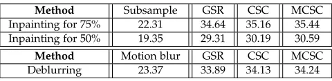
TABLE 4
Average PSNR of inpainting methods for different subsampling rates and deblurring methods.
Method Subsample GSR CSC MCSC
Inpainting for 75% 22.31 34.64 35.16 35.44 Inpainting for 50% 19.35 29.31 30.19 30.59
Method Motion blur GSR CSC MCSC
[image:7.612.60.289.381.570.2]Deblurring 23.37 33.89 34.13 34.24
Fig. 6. Comparison of different deblurring methods. (a) Original car images; (b) Motion blur images; (c) The deblurred images by CSC; (d) The deblurred images by MCSC.
4.5 Discussion of the MCSC
As shown in the above experiments, MCSC achieves a higher performance than the well-known baseline CSC. This section further discusses how a higher performance has been achieved. We illustrate the performance of MCSC and CSC based on the reconstruction error, which is an impor-tant metric to evaluate for evaluating the quality of image reconstruction. A smaller value denotes less information loss. But when we process batch images, the reconstruction error can not be used to valuate the quality of data structure. Even for a same reconstruction error, manifold structures may vary a lot. Differently we focus on both reconstruction error and structure illustration. Imposing the manifold con-straint is expected to better preserve the data structure and decrease the reconstruction loss.
Manifold Structure. In Fig.7, we plot manifold struc-tures of the input data, CSC and MCSC reconstructions on
digit ’0’ in USPS. The dataset has more than 1000images,
based on which we estimate the structures using the
Lapla-cian Eigenmaps [4] with the same iterations. Obviously,
MCSC (γ = 0.1, η = 0) achieves more similar manifold
structures as the input manifold than CSC, in comparison
with Fig.7(b), Fig.7(c) is much more similar to Fig.7(a).
The result shown in Fig.7(b) just gets worse reconstruction
actually. In addition, we plot the manifold of MCSC with
γ= 5andη= 0.5in Fig.7(d), as expected that largerγand
η can improve the smoothness of the structure. Besidesγ
andη, the number of samples also plays a crucial role in the
structure calculation, and the results in Fig.8 confirm that
larger sample sizes result in better structures. We further
select2000pairwise of digit ’6’ and evaluate the normalized
correlation between the input image and its reconstruction
in Fig.9. One can see that MCSC shows a better linear fitting
ofy=xwhile CSC has a bigger bias and variance.
Reconstruction Error.With respect to the reconstruction
error, we calculate it in the YaleB01 dataset. In Fig.10,
the MCSC demonstrates the capability of decreasing the reconstruction loss. In addition to the manifold and recon-struction error analysis mentioned above, we also evaluate the performance on dictionary compactness and feature similarity. As theorem 1 and 2 showed that the imposing manifold constraint should have the impact on compacting dictionaries and preserving feature similarity.
[image:7.612.53.293.681.740.2]normal-JOURNAL OF SELECTED TOPICS IN SIGNAL PROCESSING 8
-0.015 -0.01 -0.005 0 0.005 0.01 0.015 -0.025
-0.02 -0.015 -0.01 -0.005 0 0.005 0.01
(a)
-0.015 -0.01 -0.005 0 0.005 0.01 0.015 -0.025
-0.02 -0.015 -0.01 -0.005 0 0.005 0.01 0.015
(b)
-0.015 -0.01 -0.005 0 0.005 0.01 0.015 -0.025
-0.02 -0.015 -0.01 -0.005 0 0.005 0.01
(c)
-0.015 -0.01 -0.005 0 0.005 0.01 0.015 -0.025
-0.02 -0.015 -0.01 -0.005 0 0.005 0.01
[image:8.612.345.526.45.114.2](d)
Fig. 7. Comparison of the manifold of ’0’ samples. (a) Manifold of the original input data; (b) Manifold of CSC; (c) Manifold of MCSC (γ = 0.1, η= 0); (d) Manifold of MCSC (γ= 5, η= 0.5).
-0.03 -0.02 -0.01 0 0.01 0.02 0.03 -0.04
-0.03 -0.02 -0.01 0 0.01 0.02 0.03
(a)
-0.025-0.02-0.015-0.01-0.005 0 0.0050.010.0150.02 -0.03
-0.025 -0.02 -0.015 -0.01 -0.005 0 0.005 0.01 0.015
(b)
-0.02 -0.015 -0.01 -0.005 0 0.005 0.01 0.015 -0.03
-0.025 -0.02 -0.015 -0.01 -0.005 0 0.005 0.01 0.015
(c)
-0.015 -0.01 -0.005 0 0.005 0.01 0.015 -0.025
-0.02 -0.015 -0.01 -0.005 0 0.005 0.01
[image:8.612.64.285.49.219.2](d)
Fig. 8. Manifold of MCSC with different numbers of ’0’ samples. (a) 250 samples; (b) 500 samples; (c) 750 samples; (d) 1000 samples.
Similarity between input images
0 0.2 0.4 0.6 0.8 1 Similarity between reconstructed images 0
0.2 0.4 0.6 0.8
1 CSC
(a)
Similarity between input images
0 0.2 0.4 0.6 0.8 1 Similarity between reconstructed images 0
0.2 0.4 0.6 0.8
1 MCSC
(b)
Fig. 9. (a) The similarity correspondence between the inputs and the CSC reconstructions; (b)The similarity correspondence between the inputs and the MCSC reconstructions.
Iterations
0 10 20 30 40 50
Log Reconstruction Error 0 5 10
15 CSC
MCSC
Fig. 10. Reconstruction error analysis.
ized dictionary orthogonality function fordicas
orth(dic) = 1
K(K−1)
K
X
i=1
K
X
j=i+1
dicTi dicj,
Number of kernels
10 20 30 40 50 60 70 80 90
Orthogonality
0 0.05 0.1 0.15 0.2
0.25 CSC
[image:8.612.363.517.156.314.2]MCSC
Fig. 11. Dictionary normalized orthogonal analysis with different kernel numbers of digit ’6’.
×104
0 1 2 3 4 5 6
-2 -1 0 1 2
3 CSC
(a)
×104
0 1 2 3 4 5 6
-2 -1 0 1 2
3 MCSC
(b)
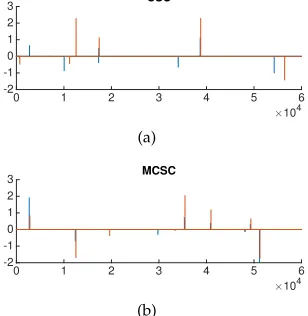
Fig. 12. (a) CSC feature maps (similarity = 0.25); (b) MCSC feature maps (similarity = 0.37); Noted that the similarity for the original image pair is 0.75.
Similarity between input images 0 0.2 0.4 0.6 0.8 1 Similarity between feature maps 0
0.2 0.4 0.6 0.8
1 CSC
(a)
Similarity between input images 0 0.2 0.4 0.6 0.8 1 Similarity between feature maps 0
0.2 0.4 0.6 0.8
1 MCSC
(b)
Fig. 13. (a) The similarity correspondence between the inputs and the CSC feature maps; (b) The similarity correspondence between the inputs and the MCSC feature maps.
where dici, the ith column of the dic, represents a
vec-torized and normalized word. We calculate the normalized orthogonality in digit ’6’ with different kernel numbers. As
shown in Fig.11, the MCSC is more compact than that of
CSC in terms of the dictionary orthogonality in most cases.
Feature Similarity. For feature similarity analysis, we plot the results of CSC and MCSC on a pair of images
(the same class) sampled from YaleB data set in Fig.12.
It can be seen that the responses using the MCSC are much more similar with a higher similarity score, but the responses using the CSC vary a lot. Selecting 2000 pairwise handwritten numbers from digit ’6’ in USPS dataset, we cal-culate the relationship between their input and feature maps using the normalized correlation, and plot their similarity
correspondence in Fig.13. The MCSC similarity in Fig.13(b)
appears better fitting toy=xthan CSC in Fig.13(a).
5
C
ONCLUSIONS [image:8.612.64.284.269.440.2] [image:8.612.316.540.368.451.2] [image:8.612.60.285.478.564.2] [image:8.612.95.258.611.681.2]insight of MCSC investigates mutual dependence among the observed and the reconstructed instances. Some theo-retical results are obtained to explain the existing Lapla-cian regularization technique in sparse coding, and the reconstruction experimental results, especially in light field, show that the proposed algorithm performs favorably better against the state-of-the-art methods based on convolutional sparse coding. In future, we will investigate the new idea in this paper for tasks of feature extractions, classifications and
tracking [39], [40].
A
PPENDIXLemma 1: If A ∈ Rn×n and B ∈ Rn×n are positive semidefinite, then
tr(AB)≤tr(A)tr(B).
Lemma 2:IfA∈ Rn×n
is positive definite andB∈ Rn×n
is positive semidefinite, then
tr(AB)≥ tr(B)
tr(A−1).
Proof of Theorem 1:In the coding update,Dis given and
Lis positive semidefinite, we have:
tr(vLvT) =tr(DzLzTDT) =tr(DTDzLzT),
where DTD is positive semidefinite, and zLzT positive
semidefinite. We then have:
tr(vLvT) +α0
N
X
n=1
K
X
k=1
kznkk22
=tr(DTDzLzT) +α0tr(zTz)
≥tr(DTDzLzT) + α
0
tr(L)tr(zLz
T
) ≥c1tr(zTLz)
and
tr(vLvT)≤tr(DTD)tr(zLzT) =c2tr(zLzT),
wherec1= 1/tr((DTD+ α
0
tr(L)I) −1)
,c2=tr(DTD).
Proof of Theorem 2: In the dictionary update step, Z
is given and L is positive semidefinite, and we have:
tr(vLvT) = tr(ZDLe De
T
ZT) = tr(ZTZ
e
DLDe
T
),where De
is a diagonal matrix, whose diagonal entries are denoted
by d, and the zero vector has the same size of vector d.
De
2
F = Nkdk
2 2. As Z
TZ
and DLe De
T
are both positive semidefinite, we have:
tr(vLvT) + (α0+β0)kdk22
=tr(vLvT) +α
0
Ntr(De
T
e
D) +β
0
N
De
2
F
≥tr(vLvT) + α
0
N tr(L)tr(DLe De
T
) +β
0
N
De
2
F
≥ tr(DLe De
T
)
tr((ZTZ+ α0
N tr(L)I)−1)
+β
0
Ntr(De
T
e
D)≥c3kdk
2 2,
and
tr(vLvT) + (α0+β0)kdk22
≤tr(ZTZ)tr(L)tr(DeDe
T
) + (α0+β0)kdk22=c4kdk
2 2,
where c3 = 1/tr((tr((ZTZ+NLα0
N tr(L)I)−1)
+ β0I)−1), c
4 =
N tr(ZTZ)tr(L) +α0+β0.
A
CKNOWLEDGMENTSThe work was supported in part by the Natural Science Foundation of China under Contract 61601466, 61672079, 61473086. The work of B. Zhang was supported in part by the Beijing Municipal Science and Technology Commission under Grant Z161100001616005. Baochang Zhang is the correspondence.
R
EFERENCES[1] K. Marwah, G. Wetzstein, Y. Bando, and R. Raskar, “Compressive light field photography using overcomplete dictionaries and op-timized projections,”ACM Transactions on Graphics, vol. 32, no. 4, p. 46, 2013.1,3,5
[2] L. Shi, H. Hassanieh, A. Davis, D. Katabi, and F. Durand, “Light field reconstruction using sparsity in the continuous fourier do-main,”ACM Transactions on Graphics, vol. 34, no. 1, p. 12, 2014.1,
3
[3] S. T. Roweis and L. K. Saul, “Nonlinear dimensionality reduction by locally linear embedding,”Science, vol. 290, no. 5500, pp. 2323– 2326, 2000.1,3
[4] M. Belkin and P. Niyogi, “Laplacian eigenmaps and spectral techniques for embedding and clustering.” inAdvances in Neural Information Processing Systems, vol. 14, 2001, pp. 585–591.1,3,4,7
[5] M. Belkin, P. Niyogi, and V. Sindhwani, “Manifold regularization: A geometric framework for learning from labeled and unlabeled examples,”Journal of Machine Learning Research, vol. 7, no. Nov, pp. 2399–2434, 2006.1,3
[6] B. Zhang, A. Perina, V. Murino, and A. Del Bue, “Sparse rep-resentation classification with manifold constraints transfer,” in Proceedings of the IEEE Conference on Computer Vision and Pattern Recognition, 2015, pp. 4557–4565.1,2,5
[7] J. Lu, G. Wang, W. Deng, P. Moulin, and J. Zhou, “Multi-manifold deep metric learning for image set classification,” inProceedings of the IEEE Conference on Computer Vision and Pattern Recognition, 2015, pp. 1137–1145.1,2
[8] F. Heide, W. Heidrich, and G. Wetzstein, “Fast and flexible con-volutional sparse coding,” inProceedings of the IEEE Conference on Computer Vision and Pattern Recognition. IEEE, 2015, pp. 5135– 5143.2,4,5,6,7
[9] P. Sermanet, K. Kavukcuoglu, S. Chintala, and Y. LeCun, “Pedes-trian detection with unsupervised multi-stage feature learning,” inProceedings of the IEEE Conference on Computer Vision and Pattern Recognition, 2013, pp. 3626–3633.2
[10] M. D. Zeiler, G. W. Taylor, and R. Fergus, “Adaptive deconvo-lutional networks for mid and high level feature learning,” in Proceedings of the IEEE International Conference on Computer Vision. IEEE, 2011, pp. 2018–2025.2
[11] Y. Zhou, H. Chang, K. Barner, P. Spellman, and B. Parvin, “Classifi-cation of histology sections via multispectral convolutional sparse coding,” inProceedings of the IEEE Conference on Computer Vision and Pattern Recognition. IEEE, 2014, pp. 3081–3088.2
[12] M. D. Zeiler, D. Krishnan, G. W. Taylor, and R. Fergus, “De-convolutional networks,” inProceedings of the IEEE Conference on Computer Vision and Pattern Recognition. IEEE, 2010, pp. 2528– 2535.2
[13] S. Gu, W. Zuo, Q. Xie, D. Meng, X. Feng, and L. Zhang, “Convo-lutional sparse coding for image super-resolution,” inProceedings of the IEEE International Conference on Computer Vision, 2015, pp. 1823–1831.2
[14] Y. Zhu and S. Lucey, “Convolutional sparse coding for trajectory reconstruction,”IEEE Transactions on Pattern Analysis and Machine Intelligence, vol. 37, no. 3, pp. 529–540, 2015.2
[15] A. Cogliati, Z. Duan, and B. Wohlberg, “Piano music transcription with fast convolutional sparse coding,” inProceedings of the IEEE International Workshop on Machine Learning for Signal Processing. IEEE, 2015, pp. 1–6.2
[16] F. D. Andilla and F. A. Hamprecht, “Sparse space-time deconvolu-tion for calcium image analysis,” inAdvances in Neural Information Processing Systems, 2014, pp. 64–72.2
JOURNAL OF SELECTED TOPICS IN SIGNAL PROCESSING 10 [18] A. Serrano, F. Heide, D. Gutierrez, G. Wetzstein, and B. Masia,
“Convolutional sparse coding for high dynamic range imaging,” inComputer Graphics Forum. Wiley Online Library, 2016, pp. 153– 163.2,7
[19] F. Heide, L. Xiao, A. Kolb, M. B. Hullin, and W. Heidrich, “Imaging in scattering media using correlation image sensors and sparse convolutional coding,”Optics Express, vol. 22, no. 21, pp. 26 338– 26 350, 2014.2
[20] X. Luo and B. Wohlberg, “Convolutional laplacian sparse coding,” inProceedings of the IEEE Southwest Symposium on Image Analysis and Interpretation. IEEE, 2016, pp. 133–136.2,3
[21] S. Gao, I. W.-H. Tsang, L.-T. Chia, and P. Zhao, “Local features are not lonely–laplacian sparse coding for image classification,” in Proceedings of the IEEE Conference on Computer Vision and Pattern Recognition. IEEE, 2010, pp. 3555–3561.2,3,5
[22] X. Wang, R. B. Li, and J. Currey, “Leveraging 2d and 3d cues for fine-grained object classification,” pp. 1354–1358, 2017.2
[23] A. Serrano, E. Garces, D. Gutierrez, and B. Masia, “Convolutional sparse coding for capturing high-speed video content,”Computer Graphics Forum, 2017.2
[24] S. Boyd, N. Parikh, E. Chu, B. Peleato, and J. Eckstein, “Distributed optimization and statistical learning via the alternating direction method of multipliers,”Foundations and TrendsR in Machine Learn-ing, vol. 3, no. 1, pp. 1–122, 2011.2,4
[25] N. Parikh, S. P. Boydet al., “Proximal algorithms.”Foundations and TrendsR in optimization, vol. 1, no. 3, pp. 127–239, 2014.2,4
[26] H. Bristow, A. Eriksson, and S. Lucey, “Fast convolutional sparse coding,” inProceedings of the IEEE Conference on Computer Vision and Pattern Recognition, 2013, pp. 391–398.2
[27] A. Ashok and M. A. Neifeld, “Compressive light field imaging,” Proceedings of SPIE, vol. 7690, no. 1, 2010.2
[28] S. D. Babacan, R. Ansorge, M. Luessi, P. R. Mataran, R. Molina, and A. K. Katsaggelos, “Compressive light field sensing,”IEEE Transactions on Image Processing, vol. 21, no. 12, pp. 4746–4757, 2012.
2
[29] Z. Xu and E. Y. Lam, “A high-resolution lightfield camera with dual-mask design,”Proceedings of SPIE, 2012.2
[30] H. Zou and T. Hastie, “Regularization and variable selection via the elastic net,” Journal of the Royal Statistical Society: Series B (Statistical Methodology), vol. 67, no. 2, pp. 301–320, 2005.3
[31] L. Yang, C. Chen, B. Zhang, and J. Han, “Adaptive multi-class correlation filters,”The Pacific-Rim Conference on Multimedia, 2016.
4
[32] R. Patel and M. Toda, “Trace inequalities involving hermitian matrices,”Linear Algebra and its Applications, vol. 23, pp. 13–20, 1979.4
[33] A. S. Georghiades, P. N. Belhumeur, and D. J. Kriegman, “From few to many: Illumination cone models for face recognition under variable lighting and pose,”IEEE Transactions on Pattern Analysis and Machine Intelligence, vol. 23, no. 6, pp. 643–660, 2001.5
[34] J. J. Hull, “A database for handwritten text recognition research,” IEEE Transactions on Pattern Analysis and Machine Intelligence, vol. 16, no. 5, pp. 550–554, 1994.5,6
[35] Y. Wu, J. Lim, and M.-H. Yang, “Object tracking benchmark,”IEEE Transactions on Pattern Analysis and Machine Intelligence, vol. 37, no. 9, pp. 1834–1848, 2015.5,7
[36] Adams, Andrewet al.[Computer Graphics Laboratory], “Stanford light field archive,” 2008,http://lightfield.stanford.edu.5
[37] J. Mairal, F. Bach, J. Ponce, and G. Sapiro, “Online learning for matrix factorization and sparse coding,” Journal of Machine Learning Research, vol. 11, no. Jan, pp. 19–60, 2010.5,6
[38] J. Zhang, D. Zhao, and W. Gao, “Group-based sparse representa-tion for image restorarepresenta-tion,”IEEE Transactions on Image Processing, vol. 23, no. 8, pp. 3336–3351, 2014.5,7
[39] B. Zhang, Z. Li, X. Cao, Q. Ye, C. Chen, L. Shen, A. Perina, and R. Ji, “Output constraint transfer for kernelized correlation filter in tracking,” IEEE Transaction on Systems, Man, and Cybernetics: Systems, vol. 47, no. 4, pp. 693–703, 2017.9
[40] B. Zhang, A. Perina, Z. Li, V. Murino, J. Liu, and R. Ji, “Bounding multiple guaasian uncertainty with application to object tracking,” International Journal of Computer Vision, vol. 118, no. 3, pp. 364–379, 2016.9
Linlin Yangreceived the B.S. and M.S. degrees in automation from Beihang University. His current research interests include signal and image processing, pattern recognition and computer vision.
Ce Li received the B.E. degree in Computer Science from Tianjin University in 2008, the M.S.and Ph.D. degrees in Computer Science from the University of Chinese Academy of Sciences in 2012 and 2015, respectively. She is currently a research assistant with China University of Mining & Technology, Beijing, China, and supported by the Natural Science Foundation of China for Youth. Her current interests include computer vision, video analysis and machine learning.
Jungong Hanis a faculty member with the School of Computing and Communications at Lancaster University, Lancaster, UK. Previously, he was a faculty member with the Department of Computer and Information Sciences at Northumbria University, UK. Dr. Han’s research interests include Multimedia Content Identification, Multi-Sensor Data Fusion, Computer Vision and Multimedia Security.
Qixiang Yereceived the B.S. and M.S. degrees in mechanical and electrical engineering from the Harbin Institute of Technology, Harbin, China, in 1999 and 2001, respectively, and the Ph.D. degree from the Institute of Computing Technology, Chinese Academy of Sciences, Beijing, China, in 2006. Since 2015, he has been a Full Professor with the University of Chinese Academy of Sciences, and was a Visiting Assistant Professor with the Institute of Advanced Computer Studies, University of Maryland at College Park, College Park, MD, USA, until 2013. He has published over 50 papers in refereed conferences and journals. His current research interests include image processing, visual object detection, and machine learning. Dr. Ye was a recipient of the Sony Outstanding Paper Award. He is a member of the IEEE.
Chen Chen received the B.E. degree in automation from Beijing Forestry University, Beijing, China, in 2009, the M.S. degree in electrical engineering from Mississippi State University, Starkville, MS, USA, in 2012, and the Ph.D. degree from the University of Texas at Dallas, Richardson, TX, USA, in 2016. He is currently a Postdoctoral Fellow with the Center for Research in Computer Vision, University of Central Florida, Orlando, FL, USA. His current research interests include com-pressed sensing, signal and image processing, pattern recognition, and computer vision. He has published over 40 papers in refereed journals and conferences in the above areas.
Xianbin Caoreceived the B.Eng and M.Eng degrees in computer ap-plications and information science from Anhui University, Hefei, China, in 1990 and 1993, respectively, and the Ph.D. degree in information science from the University of Science and Technology of China, Beijing, in 1996. He is currently a Professor with the School of Electronic and Information Engineering, Beihang University, Beijing, China. He is also the Director of the Laboratory of Intelligent Transportation System. His current research interests include intelligent transportation systems, airspace transportation management, and intelligent computation.
Baochang Zhangreceived the B.S., M.S. and Ph.D. degrees in Com-puter Science from Harbin Institue of the Technology, Harbin, China, in 1999, 2001, and 2006, respectively. From 2006 to 2008, he was a research fellow with the Chinese University of Hong Kong, Hong Kong, and with Griffith University, Brisban, Australia. Currently, he is an associate professor with Beihang University, Beijing, China. His current research interests include pattern recognition, machine learning, face recognition, and wavelets.