warwick.ac.uk/lib-publications
A Thesis Submitted for the Degree of PhD at the University of Warwick
Permanent WRAP URL:
http://wrap.warwick.ac.uk/128709
Copyright and reuse:
This thesis is made available online and is protected by original copyright.
Please scroll down to view the document itself.
Please refer to the repository record for this item for information to help you to cite it.
Our policy information is available from the repository home page.
Software for Finite Element Methods and its
Application to Nonvariational Problems
by
Lloyd Connellan
Thesis
Submitted to The University of Warwick
for the degree of
Doctor of Philosophy
Mathematics
The University of Warwick
Contents
List of Tables 4
List of Figures 6
Acknowledgments 8
Declarations 9
Abstract 10
Chapter 1 Introduction 1
1.1 A Basic Introduction to Finite Element Methods . . . 1
1.2 History of FEMs and Software Packages . . . 3
1.3 Nonvariational Problems . . . 6
1.4 Overview of Thesis . . . 10
Chapter 2 Dune-Fempy 13 2.1 Finite Element Methods in Dune-Fempy . . . 13
2.1.1 Grids . . . 16
2.1.2 Spaces . . . 18
2.1.3 Grid Functions . . . 19
2.1.4 Schemes . . . 21
2.1.5 Solving . . . 23
2.2 Alternate Solve Methods . . . 26
2.3 Model Generation . . . 35
2.3.1 Elliptic Models . . . 36
2.3.2 Integrands Models . . . 38
2.3.3 C++ Models . . . 38
2.4 Adaptive Mesh Refinement . . . 40
2.4.2 Crystal Growth . . . 47
2.5 Moving Meshes . . . 52
2.5.1 Mean Curvature Flow . . . 53
2.6 Partitioned Grids . . . 59
2.6.1 Li-ion Battery Problem . . . 59
2.7 Translating Python Code to C++ . . . 71
2.8 Virtualization . . . 73
Chapter 3 Nonvariational PDEs 77 3.1 Definition and Notation . . . 77
3.2 Existing Methods . . . 80
3.3 Minimization Method . . . 84
3.3.1 Saddle Point Formulation . . . 91
3.4 Error Analysis . . . 92
3.4.1 Error Bound for H−1 Method . . . 92
3.4.2 Numerical Demonstration ofH−1 Interpolation Error . . . . 99
3.5 Finite Element Hessian. . . 102
3.5.1 Derivation of FEH . . . 102
3.5.2 Numerical Implementation of FEH . . . 106
3.6 Numerical Implementation inDune-Fempy . . . 108
3.6.1 Numerical Setup . . . 109
3.6.2 Effectiveness and Convergence Rates . . . 116
3.6.3 Efficiency . . . 125
3.7 Nonlinear Problems . . . 129
3.7.1 Numerical Setup . . . 130
3.7.2 Effectiveness and Convergence Rates . . . 131
Chapter 4 Conclusion 137 4.1 Achieved Goals . . . 137
4.2 Future Work . . . 138
Chapter 5 Bibliography 140
Appendix A Running this code 147
Appendix B Derivation of Forchheimer Model 148
Appendix D List of Dune-Python modules 154
D.1 Grids. . . 154
D.2 Spaces . . . 155
D.3 Grid Function . . . 157
List of Tables
2.1 Runtimes for Forchheimer solve time . . . 40
3.1 Interpolation error in the Laplace case for different norms . . . 100
3.2 Interpolation error with non-constant A for different norms . . . 101
3.3 Interpolation error for a non-smooth solution with different norms . 101 3.4 Table indicating which methods are symmetric . . . 115
3.5 Levels of drop tolerance necessary for ILU . . . 116
3.6 Variational method applied to Poisson’s equation . . . 117
3.7 Nonvariational (DG) method applied to Poisson’s equation . . . 118
3.8 L2 minimization method applied to Poisson’s equation . . . 118
3.9 H−1 minimization method applied to Poisson’s equation . . . 118
3.10 L2 minimization method with H[u] . . . 119
3.11 H−1 minimization method with H[u] . . . 119
3.12 Table of EOCs for the Laplace example . . . 119
3.13 Variational method applied to the AD equation . . . 121
3.14 Table of EOCs for the AD problem . . . 121
3.15 Table of EOCs for the nonD example . . . 123
3.16 Table of EOCs for k= 1, for the nonD example . . . 125
3.17 Table of EOCs for k= 3, for the nonD example . . . 125
3.18 Condition numbers for theL2 minimization method . . . 126
3.19 Condition numbers for theH−1 minimization method . . . 126
3.20 Table of EOCs for the nonvariational p-Laplace . . . 134
3.21 Table of EOCs for the variational p-Laplace . . . 134
3.22 Table of EOCs for the simple nonlinear problem . . . 135
3.23 Table of EOCs for the Monge-Amp`ere equation . . . 136
D.1 Grids. . . 155
D.2 Gridviews . . . 155
D.4 Spaces . . . 156
D.5 Grid Functions . . . 158
List of Figures
2.1 Plot of a 2D grid for two different levels of refinement . . . 17
2.2 Node maps of two Lagrange reference elements . . . 18
2.3 The matplotlib plot of the initial function . . . 20
2.4 Plot of solutions at each level of refinement . . . 26
2.5 Plot of solution for Python-side Newton scheme . . . 29
2.6 Plot of solution with Df operator . . . 31
2.7 Plot of solution using PETSc . . . 32
2.8 Plot of solution using PETSc and a Krylov method. . . 33
2.9 Plot of solution using SNES . . . 34
2.10 The first three plots of the solution . . . 45
2.11 The second three plots of the solution . . . 45
2.12 The final three plots of the solution. . . 45
2.13 Zooming in on the re-entrant corner . . . 46
2.14 Plot of the level function of the grid . . . 46
2.15 The initial adapted grid and phase field . . . 51
2.16 The grid, phase field and temperature after the final timestep . . . . 52
2.17 The plot of the surface at three different timesteps . . . 56
2.18 Comparison of the error over time for varying levels of refinement. . 58
2.19 The domain, a cell split into three parts . . . 61
2.20 The initial plot of cand φ . . . 70
2.21 The plot after the final timestep . . . 70
2.22 Comparison of time taken between the two calcRadius methods . . . 73
3.1 Plot ofk∆(u−Ihu)k . . . 101
3.2 Plot ofk∇Nh∆(u−Ihu)k . . . 101
3.3 Plots of L2 errors for Poisson’s equation . . . 120
3.4 Plots of L2 EOCs for Poisson’s equation . . . 120
3.6 Plots of H1 EOCs for Poisson’s equation . . . 120
3.7 Plots of L2 errors for the AD problem . . . 122
3.8 Plots of L2 EOCs for the AD problem . . . 122
3.9 Plots of H1 errors for the AD problem . . . 122
3.10 Plots of H1 EOCs for the AD problem . . . 122
3.11 Plots of L2 errors for the nonD problem . . . 123
3.12 Plots of L2 EOCs for the nonD problem . . . 123
3.13 Plots of H1 errors for the nonD problem . . . 124
3.14 Plots of H1 EOCs for the nonD problem . . . 124
3.15 Comparison of the condition numbers for different methods . . . 127
3.16 Plot of the iteration count for the nonD problem . . . 128
Acknowledgments
This work has been supported by the Engineering and Physical Sciences Research
Council (EPSRC) within the MASDOC DTC at the University of Warwick.
First of all I would like to thank my supervisor Andreas Dedner for his
continual guidance in all things mathematical and computational throughout my
PhD. Without his help, often going above and beyond what I expect, I am sure this
thesis would not be possible.
Secondly I would like to thank Bj¨orn Stinner for always looking out for me
and giving me advice through my time at MASDOC. To Matteo Icardi who provided
assistance with the battery problem, I am also very grateful.
To my colleagues at MASDOC, in particular my friends Neil and Adam, I
would like to say thanks for all the support and friendly conversations over the years.
To all my friends that I have met online during this time, I would also like to offer
my thanks for their company.
Finally I wish to thank my family for always being there for me, and giving
Declarations
The work described in this thesis is the author’s own, conducted under the
supervi-sion of Andreas Dedner (University of Warwick), however we note that the software
package Dune-Fempy showcased in chapter 2 is a collaborative project with
An-dreas Dedner, Martin Nolte (University of Freiburg), Robert Kl¨ofkorn (International
Research Institute of Stavanger), Matthew Collins (University of Warwick) and other
developers. We also note that the derivation of the finite element Hessian in section
3.5was previously carried out by Andreas Dedner and Tristan Pryer (University of
Reading) in an unpublished paper (Dedner and Pryer[2013]). None of the material
contained in the thesis has been used by the author in any previous publication or
Abstract
We begin by introducing an extension to the software packageDune(a C++
based toolbox for solving PDEs with the finite element method) which has the main
objective of providing a Python user interface to it. First of all we explain how
we have structured the interface and go into some detail about the components
typical to a FEM. We then go on to demonstrate different features available in the
context of worked examples. For instance, we consider the integration of different
software packages such as PETSc and SciPy, as well as FEM features such as grid
adaptivity, moving domains, and partitioned grids. Throughout this we highlight
design decisions that are different to other similar packages and the reasoning behind
them. We conclude by demonstrating how C++ code development can be integrated
into the process and how that affects efficiency.
We go on to consider an application of this software to nonvariational PDEs.
The key contribution of this section is the development of a new method for solving
this class of problems based on minimization. We derive this method and provide
results for existence and uniqueness and error convergence. We also compare this
method to existing methods and highlight the advantages it has. We then derive a
second aspect of this method which involves a finite element version of the Hessian.
We combine these features and look at numerical results for linear nonvariational
problems. We compare the new methods along with other existing methods using
our software in terms of convergence rates and efficiency. Finally we take an
exper-imental look at solving nonlinear nonvariational problems using the finite element
Chapter 1
Introduction
1.1
A Basic Introduction to Finite Element Methods
Before talking about finite element methods (FEMs), it is only right that one first
talks of the partial differential equations (PDEs) they look to solve. PDEs have
ex-isted as a mathematical model for all manner of physical phenomena for centuries,
with equations describing how fluids flow, how heat transfers, and how sound waves
propagate. Indeed capturing the essence of how the world works around us
inher-ently requires complexity, meaning that in many cases the simpler ordinary
differ-ential equation is not enough. Yet with this complexity requires an added effort to
solve them, and often finding an analytical solution to all but the simplest PDEs is
a difficult task, and at times an impossible one. Thus in modern times we typically
look to numerical solutions and computers to solve PDEs, the most common
meth-ods being the finite difference method, the finite volume method, and of course the
finite element method.
To describe FEMs in an introductory sense, the general concept is to split up
a problem’s domain into separate smaller components (finite elements), upon which
it is much easier to approximate the solution on. By moving to a finite-dimensional
version of the function space, one concretely solves a discretized solution on each
individual element. These elements are then combined to give the whole picture of
Let us mathematically describe this method with a relatively simple example.
Let Ω⊂Rd be our domain. Then Poisson’s equationis
−∆u=f, in Ω, u= 0, on ∂Ω.
Whilst elementary, this equation sees use in many areas, including electrostatics and
fluid mechanics. Now in FEMs, the usual procedure is to obtain theweak formof the PDE by multiplying by a test functionv in a function spaceV, and integrating by parts. This results in the following equation. We wantu∈V such that
Z
Ω
∇u· ∇vdx=
Z
Ω
f vdx, ∀v∈V. (1.1)
As this weak form is a common feature of FEMs, there exists a generalized form,
a(u, v) = (f, v), ∀v∈V, (1.2) wherea(·,·) is a coercive bilinear form onV and (·,·) is theL2 inner product. In this case, the weak form of Poisson’s equation can be obtained by choosingV =H01(Ω) anda(·,·) in (1.2) to be theH01(Ω) inner product.
Following this, it is necessary to convert this equation into an algebraic
sys-tem that can be solved elementwise, i.e. to discretize it. One aspect of this is
dividing the domain Ω into a mesh of polygonal shapes{Ki}called atriangulation. Specifically, we derive an approximation Ωh such that
Ω≈Ωh = N
[
i=1
Ki.
Here Ωh is dependent onh (the mesh size) which is defined by
hK := max
x,y∈K|x−y|and h:= maxK∈Ωh
hK.
space) that approximates V. With this, we are able to write the discrete solu-tion as a linear combinasolu-tion of basis funcsolu-tions, i.e. uh(x) = PN
i=1uiϕi(x) (where
{ϕ1, . . . , ϕN} is a basis ofVh). We can also write the discrete counterpart to (1.2) as follows
a(uh, vh) = (f, vh), ∀vh ∈Vh, (1.3) Findinguh ∈Vh is known as theGalerkin method. Consequently, we can rewrite (1.3) in terms of basis functions, due to the linearity of a(·,·).
N
X
j=1
uja(ϕj, ϕi) = (f, ϕi), i= 1, . . . , N.
From here, one can form an algebraic system of equations by defining a matrixA
with entriesAij =a(ϕi, ϕj) and a vectorb with entries bi = (f, ϕi). We can then solve the linear system
Au=b,
whereu= (ui)Ni=1 are thedegrees of freedom of uh. This system of linear equations can then be solved via an appropriate algorithm, e.g. a conjugate gradient (CG)
method or generalized minimal residual (GMRES) method.
All in all this procedure allows one to consistently solve PDEs in a numerical
sense, provided they can be put into a weak form.
1.2
History of FEMs and Software Packages
Now that we have introduced what FEMs are in an elementary sense, let us expand
upon their history and development.
Among the different numerical methods for solving partial differential
equa-tions, finite element methods are one of the most popular. They have been used for
a broad range of engineering and scientific problems, with the first computational
applications originating as early as Turner et al. [1956]. Over the years there has
been an extensive amount of literature analysing FEMs in general and their uses
Just as the development of the theory of FEMs has progressed over the years,
the landscape of FEM software itself has undergone much change. As a
multidisci-plinary method involving many different techniques, the scope for which direction to
develop features is very high. Even within the realm of standard FEMs there exist a
multitude of different options available. For instance with regards to types of finite
elements, if one considersconforming finite elements (i.e. where Vh ⊂V) then one has possibilities such as the well-known Lagrange element, the H(div) conforming Brezzi-Douglas-Marini element used for instance for the elastic stress tensor, the
H(curl) conforming N´ed´elec element used in electromagnetism, and so on. Then, provided one uses an appropriate penalty method, one can further expand this to
have nonconforming elements such as theH2 Hermite (cubic) elements, the Morley (quadratic) elements used for fourth order problems, and theH1 Crouzeix-Raviart element used in Stokes flow1. In addition one can consider the mesh itself; one can
have structured grids that are more computationally efficient or unstructured ones
that allow for more flexibility. Furthermore one could have different shapes such
as squares, triangles, cubes, pyramids, hexahedrons and so on. This is all
with-out going into more complex forms of FEM such as hp-FEM (see [Melenk, 2002, §1.4.3]), spectral element methods (see [Karniadakis and Sherwin,2013,§1.2.2]) and
extended finite element methods (XFEM) (see [Fries,2008,§2]).
All in all this diversity of choice has lead to the situation of numerous
compet-ing packages that offer slightly different flavours of FEM. One preventative measure
to this has been the development of large modular software libraries that offer many
optional extensions in one place, thus forgoing the need to install different packages
for different problems. Such examples includeDune(Bastian et al. [2008]), deal.II
(Alzetta et al.[2018, accepted]), FreeFem++ (Hecht [2012]) and Elmer (Lyly et al.
[1999]). These large packages are typically written in languages such as C++ and
Fortran that are efficient for large-scale computations.
In recent years however there has been a trend towards packages that favour
usability. Such packages look to lower the learning curve for new developers and
non-computer focused researchers, allowing for more time to be spent productively
solving problems. Additionally, higher level programming languages facilitate the
use of rapid prototyping, i.e. allowing one to quickly construct new models and test
their viability without having to write an intricate program. Python and MATLAB
are both examples of commonly used languages that prioritize usability; in particular
Python has risen to become one of the most popular programming languages of
recent times (see e.g. Tio[2019]). Yet there are downsides to these languages from
the standpoint of a researcher in mathematics or engineering; namely that they are
not as efficient as their traditional counterparts in C, C++ and Java. Thus the goal
of many new packages has been to unify an interface that combines aspects of being
easier to pick up and use, without compromising the functionality and efficiency of
traditional packages.
There exist many ways to go about tackling this problem. One strategy is to
make use of more modern features of C++ (and other similar languages), such as
auto types, range-based for loops and lambda functions, to increase usability. Yet
arguably even the most user-friendly versions of these languages remain intimidating
to programming novices, due to their core design elements that cannot be changed.
A different approach is to use a language that attempts to unify usability and
efficiency in one place. Julia (Bezanson et al. [2014]) is one example of such a
language. The principal downside is the lack of popularity or wide-spread use of
any such language in comparison to Python or C.
A third alternative, one growing in popularity, is to use two languages such
as Python and C++ in the same package. The core idea behind this approach is
to use a simplified interface attached to a back end with lower level code, which
is typically achieved via the use of an automatic code generation tool like SWIG
or Cython. This tying together of front end to back end does require additional
code and maintenance of the interfacing between them, but its merit is in that it
effectively combines the best of both worlds. In particular FEniCS (Alnæs et al.
[2015]) and Firedrake (Rathgeber et al.[2017]) are examples of this kind of software.
Language (UFL) (Aln¨aes et al. [2013]), a domain-specific language (DSL) which
allows one to write variational equations directly. For instance for equation (1.1) we
have the following simple code.
Code Listing 1.1: Poisson’s equation in UFL
1 a = i n n e r ( g r a d ( u ) , g r a d ( v ) )*dx
2 b = i n n e r ( f , v )*dx
We do however note that the code generation-style approach used in FEniCS and
Firedrake does come with inherent weaknesses. In particular this generated code is
not suited to direct editing, so should a binding not exist for a feature on the Python
side, editing these generated files to add the feature on the C++ side is not an option.
Furthermore, user interactibility with the C++ interface is not prioritized, which
means porting code over to C++ for efficiency reasons or the writing of additional
features are not viable.
In the first chapter of this thesis we introduceDune-Fempy, a Dune
mod-ule that is an extension to Dune-Python (Dedner and Nolte [2018]) specifically aimed at adding high-level FEM features based on theDune-Femmodule (Dedner
et al.[2010]) to Dune. The aim of both of these packages is to bring the usability and speedier writing of code toDuneand its large array of existing modules whilst
preserving the features available to a C++ developer. In particular the structure
and functionality is designed to be analogous in many ways to Dune code,
mak-ing it less difficult to port code to C++ if necessary. Additionally, attempts to
increase usability have been made, such as library caching to reduce the runtime of
repeated computations, and integration with modern C++11/C++14 via pybind11
(seeJakob et al. [2017]) to interface between C++ and Python.
1.3
Nonvariational Problems
Continuing onwards, there exists another reason, besides the potential for
optimiza-tion, for maintaining a similar structure to Dune and other traditional C++
additional C++ code can be simply added to the interface via the use of Dune
modules and pybind11 functionality (a process that is explained in-depth inDedner
and Nolte [2018]). Considering that many interesting research topics by nature are
nontrivial, it is crucial to be able to cater for problems that do not necessarily fit
into the neat interface provided by many Python-style software packages.
Having said this, we note that there is a large range of problems that fit
into the variational framework, and by extension the myriad of numerical software
available for solving them. Indeed, since such a large variety of partial differential
equations can be put into variational (or weak) form, regardless of complexities such
as nonlinearity, it is usually not required to go beyond this scope.
There are however PDEs for which it is ill-advised, or sometimes impossible
to put into a variational form. In particular, chapter 3 of this thesis looks at the
class of PDEs that take the form
−A:D2u=f.
HereD2u is the Hessian ofu,f is a prescribed function and Ais a matrix.
In the case that the matrix A is differentiable, we note that this has an obvious equivalence with standard variational methods. For instance in the case
where A is the identity matrix, the above equation simply equates to Poisson’s equation. In such cases the above is equivalent to its variational sibling.
−∇ ·(A∇u) + (∇ ·A)∇u=f.
However we note that because of the existence of theDAterm, this cannot be done in the case whereAis not differentiable. In fact even in cases where the derivatives are close to zero, the PDE becomes advection dominated, making it probably unsuited
for conforming FEMs. Because of this possibility, in general PDEs of the above form
are classed asnonvariational.
takes the general form
F(D2u) =f(x, u, Du).
In this case F can be any kind of function acting on the second derivatives of u, which increases the scope further. In particular such nonvariational problems occur
in a variety of different contexts, for instance the Monge-Amp`ere equation (see e.g.
Guti´errez [2001]) and the Hamilton-Jacobi-Bellman equations (which have many
applications such as in economics (Cao and Wan [2009]) and engineering (Ioslovich
et al.[2009]); a review can be found inKatzourakis and Pryer[2018]).
The Monge-Amp`ere equation especially has many applications. The Dirichlet
version (in a domain Ω) takes the general form
det(D2u) =f(x, u, Du), in Ω, u= 0, on ∂Ω.
The most well-known application of this is the problem of prescribed Gauss
cur-vature on a convex domain (Trudinger and Urbas [1983], Urbas [2004]). This is a
specific example of the Monge-Amp`ere equation which takes the form
det(D2u) =K(x)(1 +|Du|2)(n+2)/2.
Another application is the mass-transfer problem (Benamou and Brenier [2000],
Evans [1997]). This originates from the Monge-Kantorovich equation, which
de-scribes the transfer of mass from one area to another. This is realized via density
functions ρ0 and ρT, and a map M between them. For a smooth one-to-one map this reduces to
det(∇M(x))ρT(M(x)) =ρ0(x)
It is then possible to prove that for some convex function Φ(x) thatM(x) =∇Φ(x), which once again returns the Monge-Amp`ere equation.
Furthermore more recently there has been an application to r-adaptivity on
grid by solving the Monge-Amp`ere equation. Another recent work (O˙za`nski[2015])
demonstrates that it can also be applied to the Navier-Stokes equations.
On the whole however, whilst due consideration has been given to specific
examples of nonvariational problems, as a class of equations themselves they have not
been studied extensively. In particular numerical methods that target this problem
are relatively few. Historically speaking, the first numerical methods developed
for tackling nonvariational problems were finite difference methods (FDMs). For
instanceOberman[2008] andLoeper and Rapetti[2005] studied the Monge-Amp`ere
equation with such an approach. The most likely reason for the popularity of FDMs
compared to FEMs for nonvariational problems is due to their compatibility with
viscosity solutions, which are a natural type of solution for nonvariational problems.
However that is not to say there is no disadvantage to FDMs, for in particular one
is only able to consider structured meshes. By considering the problem from a FEM
perspective, we open up the possibility of unstructured grids, and other useful tools
such as grid adaptivity.
One of the first papers to consider a finite element approach to
nonvaria-tional models was Lakkis and Pryer [2010], where the concept of a finite element
HessianH[u] was first introduced. This form comes from applying the distributional equation for the Hessian, i.e.
Z
Ω
D2uϕdx=− Z
Ω
∇u⊗ ∇ϕdx+
Z
∂Ω
∇u⊗nϕds.
This method has later been applied to nonlinear problems in Lakkis and Pryer
[2012], and then developed into a discontinuous Galerkin (DG) method in Dedner
and Pryer[2013]. Furthermore, we note that another DG finite element method was
proposed around the same time in I. Smears [2013], which uses an hp-FEM, and
later on an approach using a discrete version of the Hessian similar to the above was
derived inWang and Wang.
The problem has continued to see development from a FEM context. In
of−A:D2u=f.
Z
Ω
(A:D2uh)(A:D2ϕh) dx+s(uh, ϕh) =
Z
Ω
f A:D2ϕhdx, ∀ϕh ∈Vh, wheres(·,·) is a stabilization term. One singular property of this method is that the analysis is made easier by its inherent symmetry, which allows for less assumptions
to be made of the regularity of the problem. Nonetheless the fourth-order nature of
the method causes it to be less efficient numerically.
One of the main aims of chapter 3 is the development of a method that
combines the symmetric properties of the above method with the numerical efficiency
of other methods, and the use of the finite element Hessian. We also note that in
section3.2we will present a more in-depth look at the methods from the literature
and how they tie in with the method developed in this thesis.
1.4
Overview of Thesis
Let us provide an overview of the chapters of this thesis. On the whole it is divided
into two main parts, each of which is planned to become a paper in the future.
In chapter2we provide an overview of the software package Dune-Fempy,
the features it provides, and a discussion of the design decisions. We begin in
section 2.1 by introducing the interface for a simple FEM step-by-step, where we
go through the process for solving a nonlinear parabolic PDE, the Forchheimer
equation. Through this section we detail each component of the FEM and why they
are considered necessary. Following this, in section 2.2 we consider different ways
we can solve the PDE and in doing so demonstrate how the Python interface can
be fully taken advantage of. In 2.3 we instead focus on an aspect which involves
the C++ back end, by considering different ways of generating the model, and how
flexibility has been provided for C++ programmers. For a change of pace, the
remaining sections of the chapter look at additional features in the context of more
complex examples. Beginning with section 2.4, we look at two examples that use
more precision around a certain point, and the second features a time-dependent
problem that requires the grid adaption to change over time. In section 2.5 we
then consider a mean curvature example, i.e. an example where the surface evolves
over time due to a smoothing condition. For the last example, in section 2.6 we
look at a model of a Li-ion battery where the domain is divided into three separate
regions. Finally we discuss the comparison to C++ code in section 2.7, and how
virtualization has been taken into consideration in section2.8.
For chapter 3, the second part of this thesis, we consider nonvariational
problems and their discretization in Dune-Fempy. We first concretely define the
problem and corresponding notation in section 3.1. Then in section 3.2 we review
existing methods in the literature, and compare them along with a new method
proposed in this paper. We begin the analysis of this method in section 3.3, where
we formally introduce this new method based on minimization, show existence and
uniqueness, and derive a saddle point formulation. We then proceed in section3.4.1
to provide error analysis for this method in terms of a bound between the solution
and its discrete approximation. We also demonstrate that this error estimate may
be suboptimal compared to the empirical results in part3.4.2. We continue to
con-sider alterations to the numerical implementation in section3.5, where we derive a
numerical version of the Hessian, which we will use to improve the previous method
further. Following from this analysis, in section 3.6 we proceed to present the
nu-merical implementation of the previous methods, implemented in Dune-Fempy.
We compare them in the context of the linear case, considering convergence rates
and efficiency of the approaches. Finally we will look at a purely numerical
im-plementation of the nonlinear case in section 3.7, in which we look to solve the
Monge-Amp`ere method and other nonlinear problems.
To summarize things, section4 reiterates what has been achieved, and the
future directions available to continue on from this project.
We note that there are two key findings to this thesis, the first of which is
the contributions to developing Dune-Fempy2, a tool for writing and developing
finite element methods with a Python interface, based on the well-known open
source software packageDune. Dune-Fempy is the first attempt to bring Python
scripting toDune, is aimed at maintaining the flexibility of theDunemodule, and
is already used in other projects. The second key finding is the minimization method
for solving nonvariational problems, and the application of the finite element Hessian
to said method and later on to nonlinear problems.
In particular, due to the collaborative nature of the project, I also will also
emphasize the following contributions which are uniquely my own. To begin with,
in Dune-Fempy I created the initial framework for the UFL to C++ conversion
for models. Over the course of the project I have added to the underlying
infras-tructure, most notably to code involving grid functions and models. The code for
the Forchheimer example (shown in section2.1), the battery example (shown in
sec-tion2.6) and a Navier-Stokes example (not shown here) were written by me (other
examples shown were written by others and adapted to this thesis). Otherwise, all
written parts of chapter 2 (except for section 2.8) were written by me. For the
nonvariational section, the code contained within theDune-Femnv module3 is
al-most all my own, with the Monge-Amp`ere code and original Finite Element Hessian
computation written by my supervisor. In terms of the analysis, the minimization
method posed in sections 3.3 and 3.4 and the experiments in sections 3.6 and 3.7
were done by me with help from my supervisor.
3
Chapter 2
Dune-Fempy
2.1
Finite Element Methods in Dune-Fempy
When designing any software package, a natural challenge that arises is trying to
make the user interface as simple and easy to use as possible. At the same time
however, we also want to create an interface that retains all the functionality we
need.
In the context of finite element methods, this leads to the question of what
the minimal functional structure for a FEM looks like. In order to try to address this
question, we will first outline from a mathematical standpoint the general structure
we have in mind for a FEM.
To begin with, the original problem we typically want to apply a finite
ele-ment method to is a continuous PDE in some infinite-dimensional space V. First let Ω⊂Rd be a polygonal domain for our problem. We then choose a conforming
finite element space Vh = {ϕh : Ω → Rr} ⊂V, where dim Vh = N. This involves choosing a basis for Vh, which can vary depending on the problem, but typically involves piecewise polynomial functions.
Next the variational (or weak) form of the equation is defined. For the
following general form.
∂tu+L[u] =f(x), in Ω×[0, T],
u(x,0) =u0(x), in Ω,
D∇u·n=g(x), on ∂Ω×[0, T],
(2.1)
where the elliptic operatorLis defined as
L[u] :=−∇ ·D(x, u,∇u)∇u+m(x, u,∇u), (2.2) and where u0 and g are the initial and boundary conditions and n is the out-ward pointing normal. We note that we are only considering Neumann boundary
conditions here for simplicity, although Dirichlet boundary conditions are also a
possibility.
To obtain the discrete form, we begin by discretizing the PDE in time. This
results in the following method: givenu0, forn∈N0, find un+1∈Vh such that
un+1−un
∆t +LI[u
n+1] +L
E[un] =f(x, tn), (2.3) where ∆tis the time step, and LI and LE are the implicit and explicit parts of L, defined using (2.2) as
LI[u] =−∇ ·DI(x, u,∇u)∇u+mI(x, u,∇u),
LE[u] =−∇ ·DE(x, u,∇u)∇u+mE(x, u,∇u), andDI+DE =D,mI+mE =m.
The variational form is then obtained from equation (2.3) by multiplying by
a test functionϕ∈Vh and integrating by parts.
Z
Ω
un+1−un
∆t ϕ+ (DI∇u
n+1+D
E∇un)· ∇ϕ+ (mI+mE)ϕdx =
Z
Ω
f ϕdx+
Z
∂Ω
gϕds, ϕ∈Vh.
We note that in terms of the actual solving of this form, there exists potential
variation in terms of the solver used and possible nonlinearity of the problem. We
also note that this is a simple scheme for demonstration, and more complex examples
involving higher order schemes or nonconforming spaces can be easily implemented
along the same lines.
With this general form in mind, inDune-Fempywe have designed the struc-ture to take as similar a style as possible, which results in the following breakdown
of parts.
2.1.1Grid. The computational domain Ω the problem is set in.
2.1.2Space. The finite element spaceVh and type of basis functions.
2.1.3Grid functions. Functions defined on the grid that store the solutionuh and other variables.
2.1.4Scheme. The weak form of the equation, its boundary conditions, and
method for solving.
2.1.5Solving. The actual solving process and data output.
We note that there exist even further simplifications that can be made in
terms of this design choice; for instance a FEM could be distilled to simply choosing
a weak form (an operator) and a grid, and having all other things set to sensible
defaults. Additionally the code itself used to represent these methods could be
simplified to a large degree depending on the aim of the software.
Ultimately as a FEM package aimed more at extensibility and for researchers
who are willing to commit to some degree of programming, we have opted for more
complexity in some cases at the expense of this simplicity. In general this is quite a
nuanced design decision that must be made without a clearright answer.
With that in mind, for the remainder of this section we shall demonstrate
in more detail how each of these concepts are implemented in the context of a
parabolic equation derived in Kieu [2015]. A full derivation of this equation is
described in appendixB, but for the following the final form suffices.
Z
Ω 1 ∆t(u
n+1−un)ϕ +1 2K(∇u
n+1)∇un+1· ∇ϕ +1
2K(∇u
n)∇un· ∇ϕdx=
Z
Ω
f ϕdx+
Z
∂Ω
gϕds, ϕ∈Vh,
(2.5)
whereK(∇u) is a scalar function. We note that this corresponds to taking DE =
DI = 12K(∇u)I (where I is the identity matrix) and mE = mI = 0 in equation (2.4).
2.1.1 Grids
The first aspect of FEMs that we consider is probably the most fundamental aspect,
that of the grid (or mesh). Naturally, before looking at the equations we want to
solve themselves, we must look at the computational domain and how we want to
discretize it. Ideally numerical software looking to emulate FEMs should be able
to construct both simple triangulated 2D domains and more complex surfaces and
meshes.
For now we will look at a simple example. Let us suppose we have a domain
of the following form.
Ω ={(x, y)∈R2 : 0≤x≤1,0≤y ≤1}.
In creating a computational grid for this domain, it will be necessary to specify the
following things.
1. The shape of the domain (a square) and its vertices.
2. The number of elements.
3. The type of elements (e.g. square elements or triangles).
With these points in mind, we implement the grid in the following way in
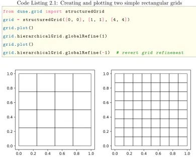
Code Listing 2.1: Creating and plotting two simple rectangular grids
1 f r o m d u n e.g r i d i m p o r t s t r u c t u r e d G r i d
2 g r i d = s t r u c t u r e d G r i d ([0 , 0], [1 , 1], [4 , 4])
3 g r i d.p l o t()
4 g r i d. h i e r a r c h i c a l G r i d . g l o b a l R e f i n e ( 1 )
5 g r i d.p l o t()
6 g r i d. h i e r a r c h i c a l G r i d . g l o b a l R e f i n e (-1 ) # r e v e r t g r i d r e f i n e m e n t
0.0 0.2 0.4 0.6 0.8 1.0 0.0
0.2 0.4 0.6 0.8 1.0
0.0 0.2 0.4 0.6 0.8 1.0 0.0
[image:29.595.122.513.113.432.2]0.2 0.4 0.6 0.8 1.0
Figure 2.1: Plot of a 2D grid for two different levels of refinement
Here we create a simple square domain by specifying two opposite corners
(0,0) and (1,1), and the number of elements in each direction (4,4). We then refine the grid and plot the results, before coarsening it again. We note that this
is a simplified example and in general grids in Dune-Fempy can additionally be
constructed via a dictionary containing vertex and element information, gmsh files or
dune grid format(dgf) files when more complexity is required, which is demonstrated
in theDune-python paperDedner and Nolte [2018]. A list of more complicated
grids and other modules is given in appendixD.
Conceptually it is worth stating that from a design standpoint, assumptions
could potentially be made to cut down on the complexity needed. For instance in
situations where the exact details are not necessary, a basic square grid could simply
(a) Second order element (b) Third order element
Figure 2.2: Node maps of two Lagrange reference elements
unclear how to make small modifications.
2.1.2 Spaces
The next key part of a FEM after constructing the grid is defining the kind of
elements we want to use, and by extension their space. In particular this is important
because the order of elements used as well as the type of element space can dictate
the solvability and the efficiency of the method.
Let us consider a simple case of Lagrange elements. Since we have a 2D
domain with a quadrilateral mesh, we consider shape functions that are 1 on each
separate node, and 0 on the others. For orders 2 and 3, the shape functions would be
quadratic and cubic polynomials respectively (as shown in figure2.2). The creation
of such a Lagrange space inDune-Fempy is done by the following code.
Code Listing 2.2: Creating a Lagrange space with polynomial basis functions
1 i m p o r t d u n e. c r e a t e as c r e a t e
2 s p a c e = c r e a t e . s p a c e (’ l a g r a n g e ’, grid, d i m r a n g e=1 , o r d e r=2 )
We note that the above space is called with two default arguments and two
keyword arguments.
’lagrange’indicates that we will use a space with Lagrange basis functions.
gridpasses in the grid we constructed previously.
order=2(optional) sets the order of the finite elements to 2 (2 is the default).
Of particular note is that the first argument corresponds to aDunediscrete space
re-alization that can come from anywhere within aDuneinstallation, provided Python bindings are created for it. For instance we could use a discontinuous Galerkin space
with orthonormal basis functions instead by using’dgonb’.
2.1.3 Grid Functions
Having defined the computational domain and function space, we look towards
functions that we may need to define, e.g. for containing the solution. In particular
we want to be able to store what initial values it can take, its value at the previous
time step and so on.
Let us begin by just considering a function for the initial condition. In
Dune-Fempy, we use Unified Form Language (UFL) (Aln¨aes et al.[2013]) to define
equations, which is essentially a human-readable way of writing a variational form.
We can also use UFL to define a simple function. To this end, we must begin by
defining a variable.
Code Listing 2.3: Creating an xvariable in UFL
1 f r o m ufl i m p o r t S p a t i a l C o o r d i n a t e
2 x = S p a t i a l C o o r d i n a t e ( s p a c e )
Here we createxas a spatial coordinate from UFL by using thespaceobject
from the previous section. The space gives UFL the dimensions of the grid and
the range space, so it knows x is two dimensional. So now for initial condition
u= 12(x20+x21)−13(x30−x31) + 1, we would have the following code. Code Listing 2.4: Creating a grid function using UFL
1 i n i t i a l = 1/2*( x[0] * *2 + x[1] * *2 ) - 1/3*( x[0] * *3 - x[1] * *3 ) + 1
Now this function can be used in a variety of ways. Let us first show how we
would compute theL2norm of the initial function. We do this using theintegrate
initialand the quadrature order5. Also note that inDune-Fempy functions are
vectors by default, so we add[0]so that it is treated as a scalar.
Code Listing 2.5: Integrating the initial data
1 f r o m d u n e. fem . f u n c t i o n i m p o r t i n t e g r a t e
2 m a s s = i n t e g r a t e (grid, i n i t i a l* *2 , o r d e r=5 )[0]
3 p r i n t( m a s s )
Output
1 1 . 8 4 0 0 7 9 3 4 5 7 0 3 1 2 5
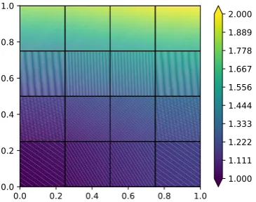
We can also plot functions fairly easily. The two main ways to do this in
Dune-Fempyare either a quick plot inmatplotlib(seeHunter[2007]), or writing to a VTK file for use in Paraview (see Ahrens et al. [2005]), which we do below,
resulting in figure2.3.
Code Listing 2.6: Plotting a function using two different methods
1 f r o m d u n e. fem . p l o t t i n g i m p o r t p l o t P o i n t D a t a as p l o t
2 p l o t( initial , g r i d=g r i d)
3 g r i d. w r i t e V T K (’ i n i t i a l ’, p o i n t d a t a= {’ i n i t i a l ’: i n i t i a l})
0.0 0.2 0.4 0.6 0.8 1.0 0.0
0.2 0.4 0.6 0.8 1.0
[image:32.595.230.413.459.603.2]1.000 1.111 1.222 1.333 1.444 1.556 1.667 1.778 1.889 2.000
Figure 2.3: The matplotlib plot of the initial function
For the vtk output the function needs to be assigned a name, which is given
by the key argument of the dictionary passed as thepointdata argument.
Note that so far we have simply evaluated the UFL expression initial
above with a discrete function, which can be created through interpolation into the
discrete function space as shown below.
Code Listing 2.7:
1 u_h = s p a c e . i n t e r p o l a t e ( initial , n a m e=’ u_h ’)
So we have created a discrete function u_h over the discrete finite element
space to contain the solution and used an interpolation over the space to assign its
initial value to the UFL expression initial. The name is used later for plotting
purposes, for example in the VTK output.
To define the weak formulation given by (2.5) we need two discrete functions,
one to store the next time step (un+1) and a second one (un) containing the approx-imation of the previous time step. We useu_h to store the former and construct a
copy,u_h_n, to store the latter.
Code Listing 2.8: Copying a discrete function
1 u _ h _ n = u_h .c o p y( n a m e=" p r e v i o u s ")
2.1.4 Schemes
InDune-Fempy, we define schemes as the object containing the weak form of the
PDE, its boundary conditions and the method used to approximate the inverse e.g.
the iterative linear solver to use. Specifically, for an operatorL:Vh →Vh∗, schemes have two main methods.
1. Apply the operator. That is to calculatewh =L[vh] given some vh∈Vh. 2. Solve the PDE. That is to compute the solutionuh toL[uh] =vh given some
vh ∈Vh∗, by using a solve method.
Remark. In the case where only the operator application is required/possible (e.g.
whenL:V →W 6=V , anoperatorobject can be constructed instead of a scheme which comes without a solve method.
Recall the parabolic equation (2.5), which we will focus on in the following
equation.
Code Listing 2.9: Setting up UFL variables to be used
1 f r o m ufl i m p o r t T e s t F u n c t i o n , T r i a l F u n c t i o n
2 f r o m d u n e. ufl i m p o r t N a m e d C o n s t a n t
3 u = T r i a l F u n c t i o n ( s p a c e )
4 v = T e s t F u n c t i o n ( s p a c e )
5 dt = N a m e d C o n s t a n t ( space , " dt ") # t i m e s t e p
6 t = N a m e d C o n s t a n t ( space , " t ") # c u r r e n t t i m e
The trial functionu and the test functionv are defined on the same space
as before. Additionally ∆t and t are defined as NamedConstant, which is simply a UFLConstantvariable that can be given a name so it can be more easily modified
later on.
Now for the equation (2.5) itself, let us prescribe the following value forK.
K(∇u) = 2
1 +p1 + 4|∇u|. (2.6)
This results in an implementation of the following form.
Code Listing 2.10: Implementing the weak form
1 f r o m ufl i m p o r t dx , grad , div , inner , s q r t
2 a b s _ d u = l a m b d a u: s q r t( i n n e r ( g r a d ( u ) , g r a d ( u ) ) )
3 K = l a m b d a u: 2/( 1 + s q r t( 1 + 4*a b s _ d u ( u ) ) )
4 a = ( i n n e r (( u - u _ h _ n )/dt , v ) \
5 + 0 . 5*i n n e r ( K ( u )*g r a d ( u ) , g r a d ( v ) ) \
6 + 0 . 5*i n n e r ( K ( u _ h _ n )*g r a d ( u _ h _ n ) , g r a d ( v ) ) ) * dx
For the exact solution we will use the following (which is consistent with the
initial data)
u(x, t) =e−2t
1 2(x
2
0+x21)− 1 3(x
3 0−x31)
+ 1 (2.7)
We can use initial to define this using some algebra, and we write a lambda
function that takestas argument.
Code Listing 2.11: The exact solution
2 e x a c t = l a m b d a t: a s _ v e c t o r ([exp(-2*t )*( i n i t i a l - 1 ) + 1])
To set the right hand side of the equation, i.e. f, we put the exact solution into the strong form of the equation (i.e. ut− ∇ ·(K(∇u)· ∇u). We also add in Neumann boundary conditions by substituting the exact solution into the boundary
term (obtained after differentiation by parts).
Code Listing 2.12: Setting up the right hand side
1 f r o m ufl i m p o r t dot, F a c e t N o r m a l , ds
2 n = F a c e t N o r m a l ( s p a c e )
3 b = i n n e r (-2*exp(-2*t )*( i n i t i a l - 1 ) \
4 - div ( K ( e x a c t ( t ) )*g r a d ( e x a c t ( t )[0]) ) , v[0]) * dx \
5 + K ( e x a c t ( t ) )*dot( g r a d ( e x a c t ( t )[0]) , n ) * v[0] * ds
Finally, having defined the weak form and right hand side, we can now set
up a scheme object which we can use to solve the PDE.
Code Listing 2.13: Creating anH1 scheme
1 s c h e m e = c r e a t e . s c h e m e (" g a l e r k i n ", a = = b , s o l v e r=’ cg ’)
The above function creates a simple Galerkin method for H1 conforming elements, with the space and equation passed in. We note thatDuneautomatically
solves nonlinear PDEs using Newton’s method so it is sufficient to simply pass in
the weak form as shown. As before we also note there exist other such premade
Duneschemes for different problems (seeD.4)
Additionally the linear solver for the method can be specified, so for this
instance we use’cg’ for a conjugate gradient method, since the PDE is symmetric
and positive definite.
Lastly we note that it is possible to explicitly define a model object to hold
the method, and we investigate the different ways of doing this in section2.3.
2.1.5 Solving
The last natural part of a FEM is the solving, which includes time loops, mesh
step, ∆t= 0.001, by assigning it in the model (using the name given to the coefficient previously).
Code Listing 2.14: Setting up time variables before the loop
1 s c h e m e . m o d e l . dt = 0 . 001
Next we write the following method for solving the problem over the time
range. Since the problem is time-dependent, we solve over a for loop with t0 = 0 andtN = 1, usingu_h_n for the old solution andu_hfor the new one.
Code Listing 2.15: Evolve method for solving in time
1 def e v o l v e ( scheme , u_h , u _ h _ n ):
2 t i m e = 0
3 e n d T i m e = 1 . 0
4 w h i l e t i m e < ( e n d T i m e - 1e-6 ):
5 s c h e m e . m o d e l . t = t i m e + 0 . 5*s c h e m e . m o d e l . dt
6 u _ h _ n . a s s i g n ( u_h )
7 s c h e m e .s o l v e( t a r g e t=u_h )
8 t i m e + = s c h e m e . m o d e l . dt
Lastly we want to have a way of computing the error. Say for instance we
want to look at the L2 and H1 errors for our computed solution. For the error we will consider the difference between an exact solution u at the final time of the simulation and our computed solution, as follows.
L2 error =
Z
Ω
|u−uh|2dx
1/2
, H1 error =
Z
Ω
|∇(u−uh)|2dx
1/2
. (2.8) We can calculate the squared norm with the following code.
Code Listing 2.16: Writing expressions for the error computed at the final time
1 e x a c t _ e n d = e x a c t ( 1 )
2 l 2 e r r o r _ f n = i n n e r ( u_h - e x a c t _ e n d , u_h - e x a c t _ e n d )
3 h 1 e r r o r _ f n = i n n e r ( g r a d ( u_h - e x a c t _ e n d ) , g r a d ( u_h - e x a c t _ e n d ) )
note that this works even though u_h is a discrete function and not a UFL term
itself, since the expression is extracted from it automatically.
We also want to compute the estimated order of convergence (EOC), to test
our method.
EOC = log(enew/eold) log(hnew/hold)
.
This is calculated by refining the grid and comparing the errors (eold and enew) to the grid sizes (hold and hnew), where the errors are computed using the error functionl2error_fn from2.16. In particular for a grid size that is being halved at
each step, we do the following after each solve step.
Code Listing 2.17: Calculating the EOCs
1 e r r o r _ o l d = e r r o r # s t o r e old e r r o r
2 e r r o r = s q r t( i n t e g r a t e (grid, l 2 e r r o r _ f n , 5 )[0]) # i n t e g r a t e
3 eoc = log ( e r r o r/e r r o r _ o l d )/log ( 0 . 5 ) # do the EOC c a l c
4 g r i d. h i e r a r c h i c a l G r i d . g l o b a l R e f i n e ( 1 ) # r e f i n e the g r i d
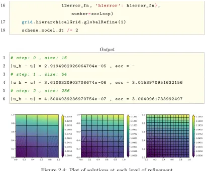
Combining these concepts into one solve method in Dune-Fempy, we have the
following program (with resulting figure2.4).
Code Listing 2.18: Solving the Forchheimer equation in time and refining the grid
1 f r o m m a t h i m p o r t log
2 e r r o r = 0
3 for e o c L o o p in r a n g e( 3 ):
4 p r i n t(’ # s t e p : ’, eocLoop , ’ , s i z e : ’, g r i d. s i z e ( 0 ) )
5 u_h . i n t e r p o l a t e ( i n i t i a l )
6 e v o l v e ( scheme , u_h , u _ h _ n )
7 e r r o r _ o l d = e r r o r
8 e r r o r = s q r t( i n t e g r a t e (grid, l 2 e r r o r _ f n , 5 )[0] )
9 if e o c L o o p = = 0:
10 eoc = ’ - ’
11 e l s e :
12 eoc = log ( e r r o r/e r r o r _ o l d )/log ( 0 . 5 )
13 p r i n t(’|u_h - u| = ’, error , ’ , eoc = ’, eoc )
14 p l o t( u_h )
16 l 2 e r r o r _ f n , ’ h 1 e r r o r ’: h 1 e r r o r _ f n},
n u m b e r=e o c L o o p )
17 g r i d. h i e r a r c h i c a l G r i d . g l o b a l R e f i n e ( 1 )
18 s c h e m e . m o d e l . dt / = 2
Output
1 # s t e p : 0 , s i z e : 16
2 | u_h u | = 2 . 9 1 9 4 9 8 2 0 2 6 0 6 4 7 8 4 e 05 , eoc =
-3 # s t e p : 1 , s i z e : 64
4 | u_h - u | = 3 . 6 1 0 6 3 2 0 9 0 3 7 0 8 6 7 4 e - 06 , eoc = 3 . 0 1 5 3 9 7 0 9 5 1 6 3 2 1 5 6
5 # s t e p : 2 , s i z e : 256
6 | u_h - u | = 4 . 5 0 0 4 9 3 9 2 3 6 9 7 0 7 5 4 e - 07 , eoc = 3 . 0 0 4 0 9 6 1 7 3 3 9 9 2 4 9 7
0.0 0.2 0.4 0.6 0.8 1.0 0.0 0.2 0.4 0.6 0.8 1.0 1.0000 1.0150 1.0301 1.0451 1.0601 1.0752 1.0902 1.1053 1.1203 1.1353
0.0 0.2 0.4 0.6 0.8 1.0 0.0 0.2 0.4 0.6 0.8 1.0 1.0000 1.0150 1.0301 1.0451 1.0601 1.0752 1.0902 1.1053 1.1203 1.1353
[image:38.595.107.516.106.447.2]0.0 0.2 0.4 0.6 0.8 1.0 0.0 0.2 0.4 0.6 0.8 1.0 1.0000 1.0150 1.0301 1.0451 1.0601 1.0752 1.0902 1.1053 1.1203 1.1353
Figure 2.4: Plot of solutions at each level of refinement
We compile a table of the errors and EOCs for additional refinement steps
and also including theH1 error below.
Elements ku−uhkL2 EOC |u−uh|H1 EOC
16 2.919e-05 - 8.917e-04
-64 3.611e-06 3.015 2.223e-04 2.000
256 4.500e-07 3.004 5.573e-05 2.000
1024 5.621e-08 3.001 1.393e-05 2.000
4096 7.031e-09 2.999 3.483e-06 2.000
2.2
Alternate Solve Methods
We carry on our explanation of different Dune-Fempy features by looking at the
back ends for spaces. Dune-fem allows one to store DoF vectors and matrices
directly based on the data structures from different linear algebra packages.
We can specify alternate storage types as follows.
Code Listing 2.19: Accessing different storage types
1 s p a c e = c r e a t e . s p a c e (’ l a g r a n g e ’, grid, d i m r a n g e=1 , o r d e r=2 ,
s t o r a g e=’ i s t l ’)
As before we construct the space, but now with the additional argument that
spec-ifies the usage of Dune-Istl (see Blatt and Bastian [2006]) as a linear algebra
backend. By default we use a very simple storage structure directly provided in
Dune-fem, consequently not requiring any additional packages. A number of
sim-ple Krylov type solvers are available. Changing thestorage argument in the
con-struction of the space makes it possible to use more sophisticated solvers (e.g., better
preconditioners or direct solvers). Available possibilities are shown in appendixD.3.
In particular one thing that we can do with certain storage methods is
inte-grate methods from SciPy (Jones et al.[2001–]) into our code. This allows for more
complex ways of writing numerical methods without the need to explicitly write it
on the C++ side. Additionally we will show that it is possible to store the degrees of
freedom in such a way that they can be treated as vectors from the NumPy package
(Oliphant [2006]) and an assembled system matrix can be stored in a SciPy sparse
matrix.
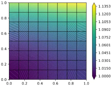
We present these methods once again via the Forchheimer example from
section2.1.
In the following we implement a simple Newton solver: given an initial guess
u0 (here taken to be zero) solve forn≥0,
un+1 =un−DS(un)(S(un)−g),
whereg is a discrete function containing the Dirichlet boundary conditions if they exist.
scheme.solve, however this time we will use the call operator on the scheme to
computeS(un) as well asscheme.assemble to get a copy of the system matrix in form of a SciPy sparse row matrix. Note that this method is not available for all
storage types. We present this alternative below, and plot the result in figure2.5.
Code Listing 2.20: Creating a class to hold a different solve method
1 i m p o r t n u m p y as np
2 f r o m s c i p y . s p a r s e . l i n a l g i m p o r t s p s o l v e
3 c l a s s S c h e m e:
4 def _ _ i n i t _ _( self , s c h e m e ):
5 s e l f . m o d e l = s c h e m e . m o d e l
6
7 def s o l v e( self , t a r g e t= N o n e):
8 # c r e a t e a c o p y of t a r g e t for the r e s i d u a l
9 res = t a r g e t .c o p y( n a m e=" r e s i d u a l ")
10
11 # c r e a t e n u m p y v e c t o r s to s t o r e t a r g e t and res
12 s o l _ c o e f f = t a r g e t . a s _ n u m p y
13 r e s _ c o e f f = res . a s _ n u m p y
14
15 n = 0
16 w h i l e T r u e :
17 s c h e m e ( target , res )
18 a b s F = m a t h .s q r t( np .dot( r e s _ c o e f f , r e s _ c o e f f ) )
19 if a b s F < 1e-10:
20 b r e a k
21 m a t r i x = s c h e m e . a s s e m b l e ( t a r g e t ) . a s _ n u m p y
22 s o l _ c o e f f - = s p s o l v e ( matrix , r e s _ c o e f f )
23 n + = 1
24
25 s c h e m e _ c l s = S c h e m e ( s c h e m e )
26
27 g r i d. h i e r a r c h i c a l G r i d . g l o b a l R e f i n e (-2 ) # r e v e r t g r i d r e f i n e m e n t
28 u_h . i n t e r p o l a t e ( i n i t i a l ) # r e s e t u_h to i n i t i a l
29 s c h e m e . m o d e l . dt = 0 . 05 # r e s e t t i m e s t e p
30 e v o l v e ( s c h e m e _ c l s , u_h , u _ h _ n )
0.0 0.2 0.4 0.6 0.8 1.0 0.0
0.2 0.4 0.6 0.8 1.0
[image:41.595.223.418.141.292.2]1.0000 1.0150 1.0301 1.0451 1.0601 1.0752 1.0902 1.1053 1.1203 1.1353
Figure 2.5: Plot of solution for Python-side Newton scheme
We can redo the above computation using a Newton-Krylov solver from
SciPy. We do this by constructing a classDfcontaining the derivative of the
opera-tor. This would normally be done within DUNE, but here we do it purely through
Python, giving figure2.6 which is identical to before.
Code Listing 2.21: Implementing a Newton-Krylov solver with SciPy
1 f r o m s c i p y . o p t i m i z e i m p o r t n e w t o n _ k r y l o v
2 f r o m s c i p y . s p a r s e . l i n a l g i m p o r t L i n e a r O p e r a t o r
3
4 def f ( x _ c o e f f ):
5 res = u_h .c o p y( n a m e=" r e s i d u a l ")
6 r e s _ c o e f f = res . a s _ n u m p y
7 x = s p a c e . n u m p y F u n c t i o n ( x_coeff , " tmp ")
8 s c h e m e ( x , res )
9 r e t u r n r e s _ c o e f f
10
11 # c l a s s for the d e r i v a t i v e DS of S
12 c l a s s Df ( L i n e a r O p e r a t o r ):
13 def _ _ i n i t _ _( self , x _ c o e f f ):
14 s e l f .s h a p e = ( x _ c o e f f .s h a p e[0], x _ c o e f f .s h a p e[0])
15 s e l f . d t y p e = x _ c o e f f . d t y p e
16 # the f o l l o w i n g c o n v e r t s a g i v e n n u m p y a r r a y
18 x = s p a c e . n u m p y F u n c t i o n ( x_coeff , " tmp ")
19 # s t o r e the a s s e m b l e d m a t r i x
20 s e l f . jac = s c h e m e . a s s e m b l e ( x ) . a s _ n u m p y
21 # r e a s s e m b l e the m a t r i x DF ( u ) g i v e n a DoF v e c t o r for u
22 def u p d a t e ( self , x_coeff , f ):
23 x = s p a c e . n u m p y F u n c t i o n ( x_coeff , " tmp ")
24 # N o t e : the f o l l o w i n g d o e s p r o d u c e a c o p y of the m a t r i x
25 # and e a ch c a l l h e r e w i l l r e p r o d u c e the f u l l m a t r i x
26 # s t r u c t u r e - no r e u s e p o s s i b l e in t h i s v e r s i o n
27 s e l f . jac = s c h e m e . a s s e m b l e ( x ) . a s _ n u m p y
28 # c o m p u t e DS ( u ) ^{- 1}x for a g i v e n DoF v e c t o r x
29 def _ m a t v e c ( self , x _ c o e f f ):
30 r e t u r n s p s o l v e ( s e l f . jac , x _ c o e f f )
31
32 c l a s s S c h e m e 2:
33 def _ _ i n i t _ _( self , s c h e m e ):
34 s e l f . s c h e m e = s c h e m e
35 s e l f . m o d e l = s c h e m e . m o d e l
36 def s o l v e( self , t a r g e t= N o n e):
37 s o l _ c o e f f = t a r g e t . a s _ n u m p y
38 # c a l l the n e w t o n k r y l o v s o l v e r f r o m s c i p y
39 s o l _ c o e f f[ : ] = n e w t o n _ k r y l o v ( f , s o l _ c o e f f ,
40 v e r b o s e=0 , f _ t o l=1e-8 ,
41 i n n e r _ M=Df ( s o l _ c o e f f ) )
42
43 s c h e m e 2 _ c l s = S c h e m e 2 ( s c h e m e )
44 u_h . i n t e r p o l a t e ( i n i t i a l )
45 e v o l v e ( s c h e m e 2 _ c l s , u_h , u _ h _ n )
46 p l o t( u_h )
We can also solvers from the PETSc package (seeBalay et al.[2018]) to solve
the problem. This can be done either through bindings available in Dune-fem or
through thepetsc4pypackage (Dalcin et al. [2011]).1
The first step is to change the storage in the space. This also requires setting
1For this to work, one must make sure that
Dunehas been configured using the same version
0.0 0.2 0.4 0.6 0.8 1.0 0.0
0.2 0.4 0.6 0.8 1.0
[image:43.595.224.417.110.259.2]1.0000 1.0150 1.0301 1.0451 1.0601 1.0752 1.0902 1.1053 1.1203 1.1353
Figure 2.6: Plot of solution with Df operator
up the scheme and discrete functions again to use the new storage structure.
We can directly use the PETSc solvers by invokingsolve on the scheme as
before. Note that to do this we must change the storage type by creating a new
space. Then we have the following code, with the same results found once again in
figure2.7.
Code Listing 2.22: Using petsc4py to solve using PETSc
1 s p a c e = c r e a t e . s p a c e (" l a g r a n g e ", grid, d i m r a n g e=1 , o r d e r=2 ,
s t o r a g e=’ p e t s c ’)
2 s c h e m e = c r e a t e . s c h e m e (" g a l e r k i n ", a = = b , s p a c e=space ,
3 p a r a m e t e r s= {" p e t s c . p r e c o n d i t i o n i n g . m e t h o d ":" sor "})
4 # f i r s t we w i l l use the p e t s c s o l v e r a v a i l a b l e in the dune-fem
p a c k a g e ( u s i n g the sor p r e c o n d i t i o n e r )
5 u_h = s p a c e . i n t e r p o l a t e ( initial , n a m e=’ u_h ’)
6 u _ h _ n = u_h .c o p y( n a m e=" p r e v i o u s ")
7 s c h e m e . m o d e l . dt = 0 . 05
8 e v o l v e ( scheme , u_h , u _ h _ n )
9 p l o t( u_h )
Next we will implement the Newton loop in Python usingpetsc4pyto solve
the linear systems. We can access the PETSc vectors by calling as_petsc on the
discrete function. Note that this property will only be available if the discrete
function is an element of a space with storage’petsc’. The methodassembleon
0.0 0.2 0.4 0.6 0.8 1.0 0.0
0.2 0.4 0.6 0.8 1.0
[image:44.595.225.416.110.259.2]1.0000 1.0150 1.0301 1.0451 1.0601 1.0752 1.0902 1.1053 1.1203 1.1353
Figure 2.7: Plot of solution using PETSc
KSP class frompetsc4py.
Code Listing 2.23: Using petsc4py and its Krylov solvers to define a Newton scheme
and solve
1 i m p o r t p e t s c 4 p y , sys
2 p e t s c 4 p y . i n i t ( sys . a r g v )
3 f r o m p e t s c 4 p y i m p o r t P E T S c
4 ksp = P E T S c . KSP ()
5 ksp . c r e a t e ( P E T S c . C O M M _ W O R L D )
6 # use c o n j u g a t e g r a d i e n t s m e t h o d
7 ksp . s e t T y p e (" cg ")
8 # and i n c o m p l e t e C h o l e s k y
9 ksp . g e t P C () . s e t T y p e (" icc ")
10
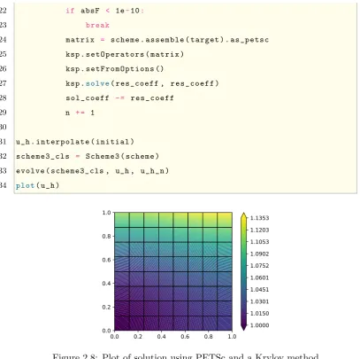
11 c l a s s S c h e m e 3:
12 def _ _ i n i t _ _( self , s c h e m e ):
13 s e l f . m o d e l = s c h e m e . m o d e l
14 def s o l v e( self , t a r g e t= N o n e):
15 res = t a r g e t .c o p y( n a m e=" r e s i d u a l ")
16 s o l _ c o e f f = t a r g e t . a s _ p e t s c
17 r e s _ c o e f f = res . a s _ p e t s c
18 n = 0
19 w h i l e T r u e :
20 s c h e m e ( target , res )
22 if a b s F < 1e-10:
23 b r e a k
24 m a t r i x = s c h e m e . a s s e m b l e ( t a r g e t ) . a s _ p e t s c
25 ksp . s e t O p e r a t o r s ( m a t r i x )
26 ksp . s e t F r o m O p t i o n s ()
27 ksp .s o l v e( r e s _ c o e f f , r e s _ c o e f f )
28 s o l _ c o e f f - = r e s _ c o e f f
29 n + = 1
30
31 u_h . i n t e r p o l a t e ( i n i t i a l )
32 s c h e m e 3 _ c l s = S c h e m e 3 ( s c h e m e )
33 e v o l v e ( s c h e m e 3 _ c l s , u_h , u _ h _ n )
34 p l o t( u_h )
0.0 0.2 0.4 0.6 0.8 1.0 0.0
0.2 0.4 0.6 0.8 1.0
[image:45.595.110.518.105.510.2]1.0000 1.0150 1.0301 1.0451 1.0601 1.0752 1.0902 1.1053 1.1203 1.1353
Figure 2.8: Plot of solution using PETSc and a Krylov method
Finally we we will use PETSc’s nonlinear solvers (thesnesclasses) directly.
Code Listing 2.24: Using petsc4py and their nonlinear solvers (SNES) directly
1 def f ( snes , X , F ):
2 i n D F = s p a c e . p e t s c F u n c t i o n ( X )
3 o u t D F = s p a c e . p e t s c F u n c t i o n ( F )
4 s c h e m e ( inDF , o u t D F )
5 def Df ( snes , x , m , b ):
6 i n D F = s p a c e . p e t s c F u n c t i o n ( x )
7 m a t r i x = s c h e m e . a s s e m b l e ( i n D F ) . a s _ p e t s c
8 m . c r e a t e A I J ( m a t r i x . size , csr=m a t r i x . g e t V a l u e s C S R () )
10 r e t u r n P E T S c . Mat . S t r u c t u r e . S A M E _ N O N Z E R O _ P A T T E R N
11
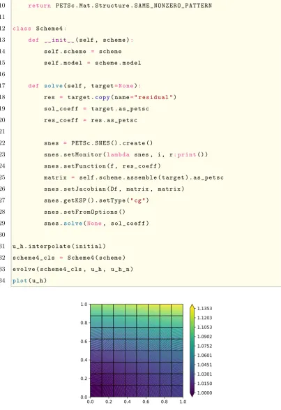
12 c l a s s S c h e m e 4:
13 def _ _ i n i t _ _( self , s c h e m e ):
14 s e l f . s c h e m e = s c h e m e
15 s e l f . m o d e l = s c h e m e . m o d e l
16
17 def s o l v e( self , t a r g e t= N o n e):
18 res = t a r g e t .c o p y( n a m e=" r e s i d u a l ")
19 s o l _ c o e f f = t a r g e t . a s _ p e t s c
20 r e s _ c o e f f = res . a s _ p e t s c
21
22 s n e s = P E T S c . S N E S () . c r e a t e ()
23 s n e s . s e t M o n i t o r (l a m b d a snes , i , r: p r i n t() )
24 s n e s . s e t F u n c t i o n ( f , r e s _ c o e f f )
25 m a t r i x = s e l f . s c h e m e . a s s e m b l e ( t a r g e t ) . a s _ p e t s c
26 s n e s . s e t J a c o b i a n ( Df , matrix , m a t r i x )
27 s n e s . g e t K S P () . s e t T y p e (" cg ")
28 s n e s . s e t F r o m O p t i o n s ()
29 s n e s .s o l v e(None, s o l _ c o e f f )
30
31 u_h . i n t e r p o l a t e ( i n i t i a l )
32 s c h e m e 4 _ c l s = S c h e m e 4 ( s c h e m e )
33 e v o l v e ( s c h e m e 4 _ c l s , u_h , u _ h _ n )
34 p l o t( u_h )
0.0 0.2 0.4 0.6 0.8 1.0 0.0
0.2 0.4 0.6 0.8 1.0
[image:46.595.110.514.109.697.2]1.0000 1.0150 1.0301 1.0451 1.0601 1.0752 1.0902 1.1053 1.1203 1.1353