warwick.ac.uk/lib-publications
Manuscript version: Author’s Accepted Manuscript
The version presented in WRAP is the author’s accepted manuscript and may differ from the published version or Version of Record.
Persistent WRAP URL:
http://wrap.warwick.ac.uk/109403
How to cite:
Please refer to published version for the most recent bibliographic citation information. If a published version is known of, the repository item page linked to above, will contain details on accessing it.
Copyright and reuse:
The Warwick Research Archive Portal (WRAP) makes this work by researchers of the University of Warwick available open access under the following conditions.
Copyright © and all moral rights to the version of the paper presented here belong to the individual author(s) and/or other copyright owners. To the extent reasonable and
practicable the material made available in WRAP has been checked for eligibility before being made available.
Copies of full items can be used for personal research or study, educational, or not-for-profit purposes without prior permission or charge. Provided that the authors, title and full
bibliographic details are credited, a hyperlink and/or URL is given for the original metadata page and the content is not changed in any way.
Publisher’s statement:
Please refer to the repository item page, publisher’s statement section, for further information.
QUADRATIC POINTS ON MODULAR CURVES
EKIN OZMAN AND SAMIR SIKSEK
Abstract. In this paper we determine the quadratic points on the modular curvesX0(N), where the curve is non-hyperelliptic, the genus is 3, 4 or 5, and the Mordell–Weil group of
J0(N)is finite. The values ofN are 34, 38, 42, 44, 45, 51, 52, 54, 55, 56, 63, 64, 72, 75, 81. As well as determining the non-cuspidal quadratic points, we give thej-invariants of the elliptic curves parametrized by those points, and determine if they have complex multipli-cation or are quadraticQ-curves.
1. Introduction
LetN be a positive integer. By the work of Mazur [26], we have a complete understanding of rational points on the modular curves X1(N); namely if X1(N)is of genus ≥1, then the
only rational points are cuspidal. Merel’s celebrated uniform boundedness theorem [28] asserts that for d ≥ 1, there is some bound Bd such that if K is a number field of degree ≤d, and N ≥Bd is prime, then the only K-rational points on X1(N) are cuspidal. There
are more precise results for small fixed degrees d. Kamienny [19] showed that if N ≥17 is prime then X1(N) has no quadratic points, and the corresponding result for cubic points
was proved by Parent [32, 33]. This has recently been extended to degrees 4, 5, 6 by Derickx, Kamienny, Stein and Stoll [10].
The situation concerning low degree points on the family X0(N) is much less happy. In
fact we only have complete results for the case of rational points. Mazur [27] proved that the only rational points onX0(N) are cusps when N is prime and greater than 163. Later,
these results were extended to composite levels and completed by Kenku (see [22] and the references therein). Results of Bars [3] and Harris–Silverman [17] assert that if X0(N) has
genus ≥2 then it has finitely many quadratic points, except for 28 values of N. A result of Aigner [1] gives all the solutions in quadratic fields to the Fermat equation x4+y4 =z4
which is isomorphic to X0(64). Recently, Bruin and Najman [5] parametrize all quadratic
points on X0(N) explicitly for those values of N where X0(N) is hyperelliptic and J0(N)
has Mordell–Weil rank 0; namely those values of N belonging to the set
{22,23,26,28,29,30,31,33,35,39,40,41,46,47,48,50,59,71}.
In this paper we focus on non-hyperelliptic X0(N) of genera 3, 4, 5 where the Mordell–
Weil group J0(N)(Q)is finite. We determine the quadratic points on these modular curves, and supply the modular interpretation of the points. In the forthcoming second part of this
Date: October 2, 2018.
2010Mathematics Subject Classification. 11G05, 14G05, 11G18.
Key words and phrases. Modular Curves, Quadratic Points, Mordell-Weil, Jacobian.
The first-named author is partially supported by Bogazici University Research Fund Grant Number 10842 and TUBITAK Research Grant 117F045. The second-named author is supported by an EPSRC LMF: L-Functions and Modular Forms Programme Grant EP/K034383/1.
work [31] we deal with those values of N for which the genus is 3, 4, 5 but J0(N)(Q) is infinite, using a version of Chabauty for symmetric powers of curves as in [36].
Lemma 1.1. The values of N for which X0(N) is non-hyperelliptic, of genus g where 3≤
g≤5 and for which J0(N)(Q) is finite are genus 3: 34, 45, 64;
genus 4: 38, 44, 54, 81;
genus 5: 42, 51, 52, 55, 56, 63, 72, 75.
LetX be a curve defined over Q. A point P ∈X is calledquadratic if the field Q(P) is a quadratic extension of Q.
Main Theorem. For the values of N listed in Lemma 1.1 the quadratic points on X0(N)
are as given in the tables of Section 8.
For the non-cuspidal quadratic points, we compute j-invariants of the elliptic curves parametrized by them. In addition, we check whether those points are related via any Atkin-Lehner involutions and decide whether or not they have complex multiplication or are Q-curves.
One motivation for this work is the current interest in the Fermat equation over quadratic fields and similar Diophantine problems. The approach via modularity and level-lowering requires the irreducibility of the mod p representation of a Frey elliptic curve defined over the given quadratic field, K say. This Frey elliptic curve often has extra level structure in the form of a K-rational 2 or 3-isogeny. If the mod p representation is reducible, then the Frey curve gives rise to a K-rational point on X0(2p) or X0(3p), and thus having a
parametrization of quadratic points is useful in establishing irreducibility for small values of p. The results of the current paper have already proved useful in that context [16].
A Theoretical Approach to the Problem. Let X/Q be a non-hyperelliptic curve of genus ≥3 withJ(Q)finite where J is the Jacobian ofX, and suppose for convenience that X has at least one rational point P0. For example X could be any of the curves X0(N)
for the values of N in Lemma 1.1. There is a straightforward theoretical method (see for instance [15]) of computing all effective degree 2 rational divisors onX, and hence all points defined over quadratic extensions, provided we are able to enumerate all the elements of J(Q). Let X(2) denote the second symmetric product of X. A
Q-rational point on X(2) can be represented by unordered pair {P1, P2} where P1, P2 are either both rational points
on X, or are defined over a quadratic field and Galois conjugate. Let D= P1+P2 and let
ι∶X(2)
(Q) →J(Q)be the map which sends D to [D−2P0]. Since X is not hyperelliptic, ι
is injective. By pulling back the finitely many points in J(Q), it is theoretically possible to determineX(2)
(Q), hence the quadratic points ofX as follows. For anyQ-rational point on X(2), the corresponding degree 2 divisor D is linearly equivalent to D′
+2P0 for some [D′]
inJ(Q) (whereD′ is rational degree 0 divisor on X). Thus, for each[D′
] inJ(Q), we need to enumerate the effective degree 2 divisors linearly equivalent to D′
+2P0. For each [D′]in
J(Q) we compute the Riemann-Roch space L(D′
+2P0). As the curve is non-hyperelliptic
the dimension of this space is either 0 or 1. If it has dimension 0 then there is no effective degree 2 divisor Dlinearly equivalent to D′
+2P0. If it has dimension 1, we let f be a non-zero element of this space, and thenD′
+2P0+div(f)is the unique effective degree 2 divisor linearly equivalent to D′
● It is often not convenient or practical to computeJ(Q) =J(Q)tors.
● Even if we can compute J(Q), it can be a large group, and the Riemann-Roch computations might not be practical for some of the more complicated elements[D′
] of J(Q).
Our Approach. For the modular curves of interest to us we first compute the rational cuspidal subgroup C = C0(N)(Q) (see below for definition) and bound its index inside J(Q), where J = J0(N). We therefore know a positive integer I such that I⋅J(Q) ∈ C. It follows that the effective degree 2 divisors D we seek satisfy [D−2P0] = I ⋅ [D′] where
[D′
] ∈J(Q). We then employ a version of the Mordell–Weil sieve to help us eliminate most possibilities for D′. Only then do we use Riemann–Roch to recover the divisors D.
Programs. The computations described in this paper have been performed using theMagma
computer algebra package [4]. Our Magma code is available with the arXiv version of the paper at https://arxiv.org/abs/1806.08192.
The Generalized Ogg Conjecture. For now let N be any positive integer. Let C0(N)
be the subgroup of J0(N)(Q) generated by classes of differences of cusps; this is known as
the cuspidal subgroup. Write C0(N)(Q) for the subgroup of C0(N) of points stable under
the action of Gal(Q/Q); this is known as the rational cuspidal subgroup, and is contained in J0(N)(Q). The Manin–Drinfeld theorem [25], [12] in fact asserts thatC0(N) ⊆J0(N)(Q)tors,
and thus C0(N)(Q) ⊆J0(N)(Q)tors. A conjecture of Ogg, proved by Mazur [26], says that
the C0(N)(Q) = J0(N)(Q)tors for N prime. A “generalized Ogg conjecture” (stated for
example in [35]) asserts that this equality holds for all positiveN. Our computations verify the conjecture for most of the values of N mentioned in the statement of Main Theorem.
Theorem 1.2. The generalized Ogg conjecture holds forN =34,38,44,45,51,52,54,56,64,81.
For recent partial results towards the generalized Ogg conjecture see [35], [23], [29], [41].
The second-named author would like to thank Martin Derickx, Steve Donnelly, Derek Holt and David Zureick-Brown for useful conversations. The authors would like to thank Ozlem Ejder and Jeremy Rouse for pointing out that X0(64) is isomorphic to the Fermat
quartic and pointing us in the direction of Aigner’s paper [1]. The authors are grateful to the referee for suggesting several significant improvements and simplifications. The authors would also like to thank theIstanbul Center for Mathematical Sciences (IMBM) for hosting their collaboration during April 2018.
2. Choices of X0(N): Proof of Lemma 1.1
Ogg [30] has shown that the values ofN for which X0(N)is hyperelliptic are
22,23,26,28,29,30,31, 33,35,37,39,40, 41,46,47,48, 50,59,71.
The genus ofX0(N)grows withN and there are only finitely many values ofN for any given
genus g. Using the explicit formula for the genus (e.g. [11, Section 3.9]), which is also the dimension formula forS2(N), we found the values of N for whichX0(N)is non-hyperelliptic
and has genus 3≤g≤5 to be
genus 3: 34, 43, 45, 64;
genus 5: 42, 51, 52, 55, 56, 57, 63, 65, 67, 72, 73, 75.
We need to decide on the values of N in this list for which J0(N) has rank 0. For this
we briefly recall standard facts about the decomposition of J0(N) as a product of abelian
varieties of GL2-type; for more details see for example Stein’s thesis [38].
Let f1, . . . , fk be representatives of the Galois-conjugacy classes of Hecke eigenforms in S2(N). Let Ki be the (totally real) number field generated by the coefficients of fi, and let di be its degree. Attached to each fi (or more precisely to its Galois-conjugacy class) is an abelian variety Ai/Q of dimension di whose endomorphism ring contains an order in Ki. In particular the rank of Ai(Q) is a multiple of di. The modular Jacobian J0(N) is
isogenous toA1× ⋯ × Ak. Thus J0(N)(Q) is finite if and only if theAi all have rank 0. Let A be any of the Ai. We writeL(A, s)for the L-function of A. The conjecture of Birch and Swinnerton-Dyer asserts that the rank ofA(Q)is equal to the order of vanishing of L(A, s) at s = 1. A deep theorem of Kolyvagin and Logachev [21] asserts that if L(A,1) ≠ 0 then A(Q) has rank 0. In fact an algorithm of Stein [38, Chapter 3] allows us to compute the exact value L(A,1)/ΩA ∈Q where ΩA is the real volume of A. Using the Magma “modular abelian varieties package”, which is an implementation by Stein of his algorithms [39], [38] we computed the ratios L(A,1)/ΩA and found them all to be non-zero for the values of N listed in the statement of Lemma 1.1. Thus we know that J(Q)is finite for those values. It remains to show that J(Q) is infinite for the remaining values 43, 53, 61, 57, 65, 67, 73; for these we claim the ranks respectively are 1, 1, 1, 1, 1, 2, 2. For each of these values of N, there is only one factor A for which L(A,1) =0, and thus the rank of J0(N)is equal to the
rank of A. For N =43, 53, 61, 57, 65 this factor A happens to be a rank 1 elliptic curve, completing the proof in those cases. For N =67 and 73 this factor is simply J0+(N) which in both cases is 2-dimensional, and it remains to show that this has rank 2 in both cases. For both values, a model for the genus 2 curve X+
0(N) is given by Galbraith [13, page 43].
Using theMagmaimplementation of Stoll’s 2-descent algorithm [40] we checked that the rank of J+
0(N) is indeed 2 in both cases.
3. Computing equations for the X0(N), Atkin–Lehner Involutions, j-maps, and cusps
Let N be such that the modular curve X0(N) has genus g ≥ 3 and is non-hyperelliptic.
Then the canonical map embeds X0(N) into projective space Pg−1 as a smooth curve of degree 2g−2, and it is this model that we work with. An algorithm for writing down the model is given by Galbraith [13]. Although equations for X0(N) for most of the N we
consider are already given by Galbraith, we needed to redo his computations so that we can explicitly construct the Atkin–Lehner involutions on the models, and also the j-map X0(N) →X(1). We start by briefly recalling Galbraith’s method.
Let S2(N) be the space of weight 2 cuspforms of level N with q-expansion coefficients
belonging to Q; this has dimension g = genus(X0(N)). The cuspforms in S2(N) can be
identified with the regular differentials on X0(N)/Q via the map f(q) ↦2πif(q)dq/q. Fix
Write
I = [SL2(Z) ∶Γ0(N)] =N∏ p∣N
(1+1 p).
By Sturm’s Theorem (e.g. [39, Theorem 9.18]), F(f0, . . . , fg−1) = 0 if and only if the q-expansion F(f0(q), . . . , fg−1(q)) = O(qr) with r = ⌊dI/6⌋ +1. Thus determining the vector space of all homogenousF of degreedsuch thatF(f0, . . . , fg−1) =0 is a straightforward linear algebra computation, and carrying this out for d∣ (2g−2) ensures that we have a system of equations that cuts out a model for X0(N) in Pg−1. For the values of N in Lemma 1.1 we
carried this out and, conveniently, found a model for X0(N)that has good reduction away
from the primes dividing N. The equations for these models are given in our tables at the end.
Next we would like to work out the Atkin–Lehner involutions on X0(N). Let m ∣ N
such that gcd(m, N/m) =1 and m≠1. The modular symbols algorithm gives the action of Atkin–Lehner operator wm as a linear operator of order 2 on S2(N) and hence as an order
2 matrix of size g×g with entries in Q. Now the linear automorphism on Pg−1 induced by this matrix restricts to the Atkin–Lehner involution wm on X0(N).
Next we describe how we obtain the map j∶X0(N) →X(1); this is not described in [13]
but similar computations are found in [2] and [15]. We start with largest divisor n∣ N for which we already know the following:
(i) equations forX0(n);
(ii) generatorsu1, . . . , us for the function field of X0(n)together with their q-expansions
at the cusp at infinity (these will in general be Laurent series); (iii) the map X0(n) →X(1).
In fact, for all values ofN that we consider, we found that theMagma“small modular curves” package gives (i), (ii), (iii) with n the largest proper divisor of N. The idea is to construct the degeneracy map X0(N) → X0(n) whence composition with X0(n) → X(1) gives the
desired j ∶X0(N) →X(1). For this it is sufficient to construct the pull-backs of u1, . . . , us toX0(N)which we denote by U1, . . . , Us. Fix 1≤i≤s and letU =Ui and u=ui. Then U is a rational function on X0(N), and hence can be written as
U = F(x0, . . . , xg−1) G(x0, . . . , xg−1)
where F,G are homogeneous in Q[x0, . . . , xg−1] of equal degree d. These satisfy
(3.1) F(f0(q), . . . , fg−1(q)) −u(q) ⋅G(f0(q), . . . , fg−1(q)) =0
where u(q) is the known q-expansion for u. Fix a degree d. Let Vd be the vector space of all homogeneous Q[x0, . . . , xg−1] of degree d and let V
′
d be the subspace belonging to the homogenous ideal generated by the equations of X0(N). Note that if H ∈ Vd′ then
H(f0(q), . . . , fg−1(q)) = 0. Thus we may think of (3.1) as a linear equation in (F, G) ∈ Vd/Vd′×Vd/Vd′, and we would like to find a non-trivial solution (for a suitable choice of d). Fixing d and a large ‘precision’ m we consider the linear system of equations
(3.2) F(f0(q), . . . , fg−1(q)) −u(q)G(f0(q), . . . , fg−1(q)) =O(q m),
in all our examples). Next we checked that the guesses U1, . . . , Us do in fact give a map X0(N) →X0(n) and we composed this with the knownX0(n) →X(1)to obtain a proposed
j-function X0(N) →X(1)which for now we denote by j′. We did not prove the correctness
of the degeneracy map X0(N) →X0(n) (which we do not use later), but we did prove the
correctness of the proposed j-function on X0(N) as we now explain. For now we think
of j and j′ as elements of the function field of X
0(N). The above procedure gives j′ =
H1(x0, . . . , xg−1)/H2(x0, . . . , xg−1)where H1, H2 are homogeneous inQ[x0, . . . , xg−1]of equal degree. Theq-expansion forj′is given byj′(q) =H
1(f1(q), . . . , fg−1(q))/H2(f1(q), . . . , fg−1(q)) and by computing enough terms we checked that j(q) −j′(q) =O(qm) some large m, where
j(q) =1
q+744+196884q+21493760q
2
+864299970q3+ ⋯
is the usual expansion of the j-function. Note that here we cannot simply apply Sturm’s Theorem to deducej=j′as we have not shown thatj−j′is a modular form (i.e. holomorphic at all the cusps of X0(N)), so we adopt a different approach. Let D and D′ be the divisor
of poles for j and j′ respectively. By [11, pages 106–107], for N >2,
deg(D) =deg(j) = N
2
ϕ(N)⋅ ∏p∣N(1− 1 p2),
where ϕdenotes the Euler totient-function. Since we know j′ we can compute D′ explicitly and we checked that deg(D′) =deg(D)in all cases. Now ifj ≠j′ then the divisor of poles for j−j′ is bounded by D
+D′ and so has degree at most 2 deg(D). But the order of vanishing of j−j′ at the cusp
∞ is at least m. Since the divisor of zeros has the same degree as the divisor of poles we deduce that m ≤2 deg(D). In all cases m exceeded 2 deg(D) +1 by a huge margin, proving j =j′.
We note in passing that theMagma“small modular curves” package is a wonderful resource, but that the justification for the modular curves data is only very briefly sketched in the
Magma handbook. Whilst we make use of this package to guess thej-function onX0(N) our
subsequent proof of the correctness of our guess is independent of it.
Finally, as we have have the j-map we can compute the cusps; these are merely the poles of j.
4. An Extension Problem for Finite Abelian Groups
Let C, A1, A2 be finite abelian groups and suppose ιj ∶ C → Aj are injective homo-morphisms. In this section we address the following question: is there is an isomorphism
ψ ∶A1 →A2 such that ψ○ι1 =ι2? This a problem we will need to address later on where
C happens to be the rational cuspidal subgroup of J0(N) and A1, A2 are candidates for
J0(N)(Q)tors obtained from local information. Let p be a prime, and write C[p∞], A1[p∞]
and A2[p∞]for thep-power torsion in C, A1,A2. Clearly the question has a positive answer
if and only if the corresponding question for C[p∞], A
1[p∞] and A2[p∞] has a positive
an-swer for every prime pdividing the orders of the groups A1,A2. Thus we may suppose that
C, A1, A2 are p-power torsion finite abelian groups for some prime p.
Of course the question has a negative answer ifA1 is not isomorphic to A2. Thus first we
make sure thatA1, A2 are isomorphic and write down an explicit isomorphismψ0∶A1 →A2.
A1 →A2; any such isomorphism will be a composition of ψ0 with an automorphism of A2.
These steps can be carried out using for example algorithms explained in [7] and implemented in Magma. Now we may simply test the isomorphisms ψ ∶ A1 →A2 and see if there is one
that satisfies ψ ○ι1 = ι2. This strategy does provide a theoretical answer to our question.
In our application we have found it impractical as the automorphism groups Aut(Ai) are enormous. As an illustration we point out that if A = (Z/pZ)n, then Aut(A) ≅ GLn(Fp). Thus whilst #A=pn, we have # Aut(A) = (pn−1)(pn−p)⋯(pn−pn−1).
WriteBi =Ai/ιi(C)and letπi ∶Ai →Bi be the quotient maps. Any isomorphismψ ∶A1→
A2 satisfying ψ○ι1 =ι2 induces an isomorphism µ∶B1 →B2 that makes the diagram (4.1)
commute, where the two rows are exact.
(4.1)
0 ÐÐÐ→ C ÐÐÐ→ι1 A1 π1
ÐÐÐ→ B1 ÐÐÐ→ 0
∥ ψ
× × × Ö
µ×× × Ö 0 ÐÐÐ→ C ÐÐÐ→ι2 A2
π2
ÐÐÐ→ B2 ÐÐÐ→ 0
Thus we know that our question has a negative answer if B1, B2 are not isomorphic. We
suppose that they are isomorphic and we enumerate all isomorphisms µ ∶ B1 → B2 (by
computing the automorphism group of B2). In our application the groups Bi tend to be rather small and so there are far fewer isomorphisms B1 →B2 than isomorphisms A1 →A2.
For each µ we now ask the following: is there an isomorphism ψ ∶A1 →A2 that makes the
diagram (4.1) commute. In essence we can interpret both exact sequences as extensions of B2 by C and we are asking if they are equivalent extensions. However we are interested
in answering this question in the category of finite abelian groups and would like to avoid computing Ext(B2, C)(which classifies all extensions of B2 byC including the non-abelian
ones) as well as avoiding the computation of the images of the two sequences in this group. The following proposition gives us an efficient way of answering the question in the category of finite abelian groups.
Proposition 4.1. Let
0→CÐι→i Ai Ðπ→i Bi →0
be exact sequences of finite abelian groups, for i = 1, 2. Let µ ∶ B1 → B2 be an
isomor-phism. Let x1, . . . , xr be any elements of A1 such that A1 is generated by ι1(C)together with
x1, . . . , xr. Let y1, . . . , yr∈A2 satisfy π2(yj) =µ(π1(xj)) for j =1, . . . , r (these must exist as π2 is surjective). Write x= (x1, . . . , xr) ∈ Ar1 and y= (y1, . . . , yr) ∈ Ar2. Let A =Zr×C. Let
τ ∶ A →A1 be given by
τ(m, c) =m⋅x+ι1(c) for m∈Zr and c∈C;
here(m1, . . . , mr) ⋅ (x1, . . . , xr) is shorthand for the linear combinationm1x1+ ⋯ +mrxr. Let (n1, c1), . . . ,(ns, cs) be a set of generators for the kernel of τ. Define a homomorphism
η∶Cr→As2, t↦ (ι2(n1⋅t), . . . , ι2(ns⋅t)),
and let
κ= (n1⋅y+ι2(c1), . . . ,ns⋅y+ι2(cs)) ∈As2.
Proof. Supposeκbelongs to the image of η. We will show the existence of a homomorphism ψ ∶ A1 →A2 making the diagram (4.1) commute. It then easily follows that ψ must be an
isomorphism (this fact is known as the short-five lemma). As κ is in the image of η, so is −κ. Thus there is somet= (t1, . . . , tr) ∈Cr such that
(4.2) nj⋅y+ι2(cj) = −ι2(nj⋅t), j =1, . . . , s.
Let
σ∶ A →A2, σ(m, c) =m⋅y+ι2(m⋅t) +ι2(c), for m∈Zr and c∈C.
Recall that (n1, c1), . . . ,(ns, cs) are generators for the kernel of τ ∶ A →A1. Condition (4.2) ensures that the kernel of τ is contained in the kernel of σ ∶ A → A2. Thus we obtain a well-defined homomorphism A/Ker(τ) → A/Ker(σ) → A2. By hypothesis A1 is generated
byx1, . . . , xr and ι1(C)thus τ ∶ A →A1 is surjective. We let ψ be the composition
A1
∼
Ð→ A/Ker(τ) → A/Ker(σ) →A2.
It follows from the definitions of τ and σ that ψ sends ι1(c) to ι2(c) for any c ∈ C, and
sends xj toyj+ι2(tj)for j=1, . . . , r. In particular, the left-hand square of (4.1) commutes. Moreover
π2(ψ(xj)) =π2(yj+ι2(tj)) =π2(yj) =µ(π1(xj))
where the last equality comes from our original definition of the yj. Sincex1, . . . , xj together with ι1(C) generate A1 the right-hand square of (4.1) also commutes.
Now conversely suppose there is an isomorphismψ ∶A1 →A2making (4.1) commute. Thus
π2(ψ(xj)) =µ(π1(xj)) =π2(yj). By the exactness of the bottom row, ψ(xj) =yj+ι2(tj) for some tj ∈C. Now let (ni, ci) be as in the statement of the theorem. Thus ni⋅x+ι1(ci) =0. Letting t= (t1, . . . , tr)and applying ψ we have
ni⋅y+ι2(ni⋅t) +ι2(ci) =0.
It follows that κ=η(−t)completing the proof.
5. The Mordell–Weil Information
Now letN be one of the values ofN in Lemma 1.1. In this section we explain how compute the structure of the rational cuspidal subgroupC0(N)(Q)as well as deducing a small integer
I such that I⋅J0(N)(Q)tors⊆C0(N)(Q).
genus 5 cases. However Magma computations in Pic0(X/F)are much more efficient when F is a finite field, and in fact the Magma implementation of Hess’ algorithm does compute the structure of Pic0(X/F) ≅ J(F)in all the cases of interest to us, where F is a finite field of characteristicp, withpa prime of good reduction for our modelX=X0(N). Our strategy is to carry out as much of the computations over finite fields as possible. A particularly useful fact for us is the following. Let X be curve defined over a number field K, let p> 2 be a rational prime, let p be a prime of K above p of ramification degree 1 and of good reduc-tion for X. Then a theorem of Katz [20, appendix] asserts that the composition of natural maps J(K)tors↪J(K) →J(Fp)is an injection. In particular we may identify J(K)tors as a
subgroup of J(Fp).
5.2. A closer look at the rational cuspidal subgroup. To ease notation we shall write X andJ forX0(N)andJ0(N). Letd2 be the largest square divisor ofN, and letK =Q(ζd) be the d-th cyclotomic field. The cusps of X are all defined over K. Let these beP0, . . . , Pk with P0 defined over Q (there are always at least two rational cusps: the ∞cusp and the 0 cusp). HenceforthP0 will be the base-point for the Abel–Jacobi map X→J. Let
D = k ∑ i=1
Z⋅ (Pi−P0).
This is the subgroup of Div0(X/K)supported on the cusps. Write G=Gal(K/Q); this acts naturally onD and we denote byDG the subgroup of divisors that are stable underG(these are the degree 0, Q-rational divisors supported on the cusps). Write
C′
= {[D] ∶ D∈ DG}
for the image of D in J(Q). NowG also acts on the subgroup
E = k ∑ i=1
Z⋅ [Pi−P0]
of J(K). The group EG⊂J(Q) is precisely the rational cuspidal subgroupC =C0(N)(Q). Of course C′ is contained inside C, and it is natural to ask if they are equal.
Lemma 5.1. Let N be one of the values in Lemma 1.1. Then C = C′. In other words,
every degree 0rational divisor class supported on the cusps is the class of a degree0 rational divisor supported on the cusps.
The lemma will bring some simplifications to our later computations comparing C with the torsion subgroup. We note in passing that as X(Q) ≠ ∅, it is known [34, Section 3] that every degree 0 rational divisor class is the class of a degree 0 rational divisor. However, applying this to a degree 0 rational divisor class supported on the cusps does yield a degree 0 rational divisor defining the same class, but that divisor need not be supported on the cusps.
Proof of Lemma 5.1. Since we have the cusps as points onX with coordinates inK, we can compute EG.
Now letp∤2N be a rational prime and letp be a prime ofK above p. In particular p∤d and so p is an unramified prime. It follows from the aforementioned theorem of Katz that the reduction modulo p map π ∶ J(K)tors→J(Fp) is injective. For σ∈G we let
It follows from the injectivity of π that [D]σ= [D] if and only if µ
σ(D) =0. Let
F = ⋂ σ∈G
Ker(µσ).
This is precisely the subgroup of D of divisors representing rational divisor classes. The image of F in J(Fp) lands in fact inside J(Fp) and is isomorphic to C. The image of EG inside J(Fp) is contained in the image of F and is isomorphic to C′. For each N we made a suitable choice of p, p and computed both these images and checked that they are equal. ThusC =C′.
Having established the equalityC=C′, we have another more convenient way of thinking of C. Let P0, . . . ,Pr be the cusp places on X/Q, with P0 = P0 as before a cusp place of degree 1. From the equality C=C′ we now know that
C = r ∑ i=1
Z(Pi−deg(Pi) ⋅ P0).
Thus for any p ∤ N, to compute the image of C in J(Fp) we merely take the subgroup generated by the reductions of Pi−deg(Pi) ⋅ P0..
5.3. The real torsion subgroup of J0(N). LetN be a positive integer and let g be the
genus ofX0(N). The torsion subgroup ofJ0(N)(C)is isomorphic to(Q/Z)2g. So the group J0(N)(Q)tors isomorphic to a product of Z/d1Z× ⋯ ×Z/d2gZ with d1 ∣d2∣ ⋯ ∣d2g. However J0(N)(Q)torsis contained in the torsion subgroup ofJ0(N)(R)and we can use this to deduce
thatd1, . . . , dg∈ {1,2}, and often in fact to cut down the number of possibilities ford1, . . . , dg as we shall see below.
We shall need the following theorem of Snowden [37], which tells us the number connected components of X0(N)(R).
Theorem 5.2 (Snowden). Let N be a positive integer. If N is a power of2 thenX0(N)has
one real component. Otherwise let n be the number of odd prime divisors of N. Let =1 if 8∣N and =0 otherwise. Then X0(N) has 2n+−1 real components.
We shall also need the following well-known theorem, which perhaps first appears in a paper of Gross and Harris [14].
Theorem 5.3. Let X/R be a smooth curve with X(R) ≠ ∅. Let g be the genus of X, m the
number of its real components and J its Jacobian. Then
J(R) ≅ (R/Z)g× (Z/2Z)m−1.
Thus
J(R)tors≅ (Q/Z)g× (Z/2Z)m−1.
Proof. By [14, Proposition 3.2], the number of connected components of J(R)is 2m−1. The
theorem follows from [14, Section 1].
5.4. Computing the possibilities for J0(N)(Q). We return toN being one of the values
in Lemma 1.1, and we continue writing X =X0(N), J =J0(N) and C=C0(N)(Q). Recall
that J(Q) is finite for all values of N we are considering. Thus C ⊆ J(Q)tors = J(Q). In
under the reduction mod p map, and ι is the restriction of the mod p map to C. Thus we know that for some ι∈ A′
p, we have a commutative diagram
(5.1) C
ι
//J(
Q)
red
µ
A //J(Fp)
whereµis an isomorphism. Letgbe the genus ofX, andmbe the number of real components of J which maybe computed from Theorem 5.2. By Theorem 5.3, we know that
J(Q) ≅Z/d1Z× ⋯ ×Z/dkZ, d1∣d2∣ ⋯ ∣dk
where k ≤g or g+1≤k≤g+m−1 and d1, . . . , dk−g ∈ {1,2}. Thus we eliminate from A ′ p all ι∶C→A where the isomorphism class ofA is incompatible with this information, to obtain a subsetAp.
Let p1, . . . , ps be distinct primes ∤ 2pN. We let Ap;p1,...,ps be the set of ι ∶C → A in Ap
such that the following holds: for each p′∈ {p
1, . . . , ps} there is some ι′ ∶C→A′ in Ap′ and an isomorphism ψ∶A→A′ making the diagram
C
ι′
&
&
ι // A
ψ
A′
commute. The existence of the isomorphism can be efficiently decided using the method explained in Section 4. It is clear that there must be some ι ∶ C → A in Ap;p1...,ps and an
isomorphism µ∶ A→J(Q) such that the diagram (5.1) commutes. Observe that Ap;p1,...,ps must contain some ι0 ∶C→A0 where A0 is the image of C under the reduction mod p map.
Our hope is to find suitablep,p1, . . . , pssuch thatAp;p1,...,ps contains precisely one element,
in which case this is necessarily ι0, and we can then deduce thatJ(Q) =C. In any case we know that J(Q)/C is isomorphic to the cokernel of some ι in Ap;p1,...,ps which allows us to
deduce a positive integer I such that I⋅J(Q) ⊆C.
Lemma 5.4. Let N be one of the values given in Lemma 1.1. Then C and J(Q)/C are as
given in the tables of Section 8.
Proof of Lemma 5.4 and Theorem 1.2. We wrote a Magma script which for each value of N computed Ap;p1,...,ps where p is the smallest rational prime not dividing 2N, and p1, . . . , ps
are the primes ≤ 17 not dividing 2pN. This allowed us to deduce the information in the tables except for two cases, where N =45, 64. For those two cases were able to improve on the information given in by this method and deduce that J(Q) =C. We explain this below
in Sections 5.5 and 5.6.
5.5. The Mordell–Weil Group for J0(45). Let N =45. The procedure explained above
tells us that C≅Z/2Z×Z/4Z×Z/8Z, and
We would like to show that J(Q) = C, and for this it is enough to show that J(Q)[2] = C[2] = (Z/2Z)3. However for all primes p∤N we triedJ(Fp)[2] = (Z/2Z)6 or(Z/2Z)4, and so it does not seem to be possible to prove the desired conclusion using reduction modulo primes. Instead we will compute the entire mod 2 representation of J
ρJ,2 ∶ Gal(Q/Q) →Sp6(F2)
and use this to deduce that J(Q)[2] = (Z/2Z)3.
The curve X=X0(45) is a smooth plane quartic. Our model for it is
X ∶ x3z−x2y2+xyz2−y3z−5z4 =0
in P2. A procedure for computing the mod 2 representation of Jacobians of smooth plane
quartics is explained by Bruin, Poonen and Stoll [6, Section 12] and we apply that method to our situation. We wrote down the equations for the 28 bitangents to X. We found that the field of definition of these bitangents isK =Q(
√
−3,√5) and so Q(J[2]) =K. In particular ρJ,2 factors through Gal(K/Q), and we continue to denote the corresponding representation Gal(K/Q) → Sp6(F2) by ρJ,2. Each bitangent L meets X in a divisor (L.X) which has
the form 2DL where DL is an effective degree 2 divisor. We wrote down the set Σ of all quadruples{L1, . . . , L4}such thatDL1+ ⋯ +DL4 ∼2ωX, whereωX is the canonical divisor on
X. As predicted by [6] this set Σ has cardinality 315. Next we construct the graphG whose vertices are the quaruples Q∈Σ, and where Q≠Q′ are connected by an edge if and only if Q∩Q′ ≠ ∅. We computed the automorphism group Aut(G) using Magma (this routine is an implementation of the algorithm described in [24]), and found it to be isomorphic to Sp6(F2) as predicted by [6]. Now the action of Gal(K/Q)on the lines naturally gives a representation Gal(K/Q) →Aut(G) ≅Sp6(F2), and this is precisely ρ=ρJ,2 ∶Gal(K/Q) →Sp6(F2) (up to
conjugation inside Sp6(F2)). Let τ1, τ2, τ3 be the elements of Gal(K/Q) satisfying
{τ1( √
−3) =√−3 τ1(
√
5) = −√5 , { τ2(
√
−3) = −√−3 τ2(
√
5) =√5 , τ3 =τ1τ2.
Write Mi=ρ(τi). We found that
M1=
⎛ ⎜ ⎜ ⎜ ⎜ ⎜ ⎜ ⎜ ⎝
1 0 0 0 0 0 0 0 1 1 0 1 0 1 0 1 0 1 0 0 0 1 1 1 0 0 0 0 0 1 0 0 0 0 1 0 ⎞ ⎟ ⎟ ⎟ ⎟ ⎟ ⎟ ⎟ ⎠
, M2=
⎛ ⎜ ⎜ ⎜ ⎜ ⎜ ⎜ ⎜ ⎝
1 0 0 0 0 0 1 0 0 0 0 1 1 0 0 1 1 1 1 1 0 1 0 1 1 0 1 1 0 1 1 1 0 0 0 0 ⎞ ⎟ ⎟ ⎟ ⎟ ⎟ ⎟ ⎟ ⎠
, M3 =
⎛ ⎜ ⎜ ⎜ ⎜ ⎜ ⎜ ⎜ ⎝
1 0 0 0 0 0 1 0 0 0 1 0 1 0 0 1 0 0 1 0 1 0 0 0 1 1 0 0 0 0 1 0 1 1 0 1 ⎞ ⎟ ⎟ ⎟ ⎟ ⎟ ⎟ ⎟ ⎠ .
WriteVi=Ker(Mi−I)whereI∈Sp6(F2)is the identity matrix. ThusVi is isomorphic to the subspace of J[2] fixed byτi. We found that V1, V2, V3 are 4-dimensional, butV1∩V2∩V3 is
5.6. The Mordell–Weil group for J0(64). Let N =64. The procedure explained above
gives us
C ≅Z/2Z× (Z/4Z)2,
and
J(Q) ≅Z/2Z× (Z/4Z)2, or (Z/4Z)3.
We want to show that J(Q) = C. For this it is enough to show that J(Q)[4] = C. The cusps of X0(64)are defined over K =Q(ζ8) =Q(i,
√
2). Let L=Q( √
2). Let G=Gal(K/Q) and H=Gal(K/L) ⊂G. The method explained in Subsection 5.2 computes C0(64)(K)(the
full cuspidal group) and then C = C0(64)(Q) is obtained by taking G-invariants. Instead we take H-invariants to obtain C0(64)(L) and find C0(64)(L) ≅ (Z/4Z)3. Note that this is contained inJ(L)[4]. However, from Theorems 5.2 and 5.3 we know thatJ(R)[4] ≅ (Z/4Z)3. As L ⊂R we deduce J(L)[4] = C0(64)(L) ≅ (Z/4Z)4. Hence J(Q)[4] ⊆ C0(64)(K). Now
taking G-invariants we have J(Q)[4] ⊆C0(64)(K)G=C. This proves that J(Q) =C.
6. The Mordell–Weil Sieve
LetX/Q be a curve of genus ≥3 with JacobianJ, and supposeX is not hyperelliptic. In this section we explain a version of the Mordell–Weil sieve for quadratic points on X, under the assumption that J(Q) has rank 0, but without assuming full knowledge of J(Q). Let P0 ∈X(Q). We use this to fix a map X(2)→J given by D↦ [D−2P0].
Let K be a (known) set of rational effective divisors of degree 2. Let G be a subgroup of J(Q) and I a positive integer such that I ⋅J(Q) ⊆ G; again we assume that G and I are known, but that J(Q) is perhaps unknown. We will use our partial knowledge of the Mordell–Weil group to sieve for unknown rational effetive degree 2 divisors. Let p≥3 be a prime of good reduction for X. Let
Vp= {D˜ ∈X(2)(Fp) ∶ D∈ K}, Up =X(2)(Fp) ∖ Vp.
Lemma 6.1. Let D′
∈X(2)
(Q) and suppose D˜′
∈ Vp. Then D′∈ K.
Proof. By defintion of Vp we have ˜D′ =D˜ for some D∈ K. Thus the divisor class [D′−D] is in the kernel of the reduction map J(Q) → J(Fp). However, J(Q) is torsion. By the injectivity of torsion [20, appendix] under mod preduction we conclude that D∼D′. It will be enough to show that D= D′. Suppose otherwise, then the Riemann–Roch space L(D) has dimension at least 2. Let f ∈ L(D) be a non-constant function. Then f ∶X →P1 has degree 2 contradicting the assumption that X is non-hyperelliptic.
Lemma 6.2. Letp1, . . . , pr be primes ≥3of good reduction forX. Let φi ∶G→J(Fpi)be the composition for the inclusion G↪J(Q) with the reduction modulo pi map J(Q) → J(Fpi). If D∈X(2)
(Q) ∖ K then
(6.1) I⋅ [D−2P0] ∈ r ⋂ i=1
φ−1
i ({I⋅ [D˜−2 ˜P0] ∶ D˜ ∈ Upi}).
Proof. SinceI⋅J(Q) ⊆G, we know thatI⋅ [D−2P0] ∈G. By Lemma 6.1, we know that the
7. Proof of Main Theorem
Let N be one of the values in Lemma 1.1. Thanks to Lemma 5.4, we know a set that contains all the possibilities forJ(Q)/C. We takeI to be the least common multiple of the exponents of these groups. Thus I⋅J(Q) ⊆ C. In each case we know the rational points on X and thus we have some collection K0 of effective degree 2 divisors of the form P +Q
whereP,Qare rational points onX. We searched for quadratic points onP onX and took K to be the union of K0 together with P +Pσ where P runs through the quadratic points
we have found, and Pσ is Galois conjugate of P. We took K as our known set of degree 2 divisors on X. We then applied Lemma 6.2 for a suitable choice of primes p1, . . . , pr ≥3 of good reduction, and withG=C, to deduce a subset ofS ⊆J(Q)given by (6.1) that contains the possibilities forI⋅ [D−2P0] for D∈X(2)(Q) ∖ K. We found, forN ≠42, 72, that S = ∅,
and thus X(2)
(Q) = K. The two values N =42, 72 needed virtually identical arguments to complete the proof thatX(2)
(Q) = K. We illustrate this now by giving a detailed account of the computation forX0(72).
The curve X0(72) has 8 cusps of degree 1 and 4 cusp pairs defined over quadratic fields.
Let these be P0, . . . , P7 and Qi, Q′i wherei=1,2,3,4 and Qi, Q′i are Galois conjugates. The modular symbols algorithm shows that J0(72) is isogenous to a productE12×E22×E3 where
E1, E2, E3 are respectively the elliptic curves with Cremona labels 24A1, 36A1, 72A1. As
these three elliptic curves have rank 0 so doesJ0(72). We write X=X0(72)and J=J0(72).
Let K consist of the known degree 2 effective rational divisors: Qi+Q′i for i=1, . . . ,4 and Pi+Pj where 0≤i, j≤7. Thus K has 40 elements. From our tables in Section 8 we have
C =Z/2Z×Z/4Z×Z/12Z×Z/12Z, J(Q)/C=0 or Z/2Z.
We take G = C and I = 2. We applied Lemma 6.2 with just one prime p = 5. We found that #X(2)
(F5) = 64. Of these 64 divisors, 40 are reductions of elements in K and the
2×5 matrix A(D)˜ has rank 2 for all 40. Thus #U5 has 24 elements. However, only two
elements of the set {2[D˜ −2 ˜P0] ∶ D˜ ∈ U5} are in the image of φ5 ∶ G ↪J(F5). We let A1, A2 be their preimages in G (which we represent as divisors of degree 0 on X). Thus if
D∈X(2)
(Q) ∖ K then 2D∼Ai+4P0. We found that the Riemann–Roch spaces L(Ai+4P0)
are both 2-dimensional. Suppose i = 1 and let f, g be a Q-basis for L(A1 +4P0). Thus
2D= A1+div(αf +βg) for some (α, β) ∈ P1(Q). We consider the 1-dimensional family of 0-dimensional subschemesA1+div(αf+βg)ofX(2)parametrized by(α, β) ∈P1. Computing
and factoring the discriminant of this subscheme (as a homogeneous expression inα,β) shows that none of the elements of this 1-dimensional family has the form 2D with D ∈X(2)
(Q). This shows that no element D∈X(2)
(Q)satisfies 2D∼A1+4P0. An identical argument also
allows us to deduce a contradiction for i=2. This shows thatX(2)
(Q) = K. Therefore there are no non-cuspidal quadratic points on X0(72).
Remark. In the above computation for X0(72) we have applied the Mordell–Weil sieve
with just one prime p=5. In fact we have found in this case that using additional primes does not allow us to eliminateA1,A2 using just the Mordell–Weil sieve and it is instructive
to ponder the reason for this. In both cases i=1, 2, the discriminant mentioned above has three quadratic factors which give divisorsDbelonging toX(2)
(Q( √
−1)),X(2) (Q(
√
3))and X(2)
(Q( √
the fields Q( √
−1), Q( √
3), Q( √
−3) it follows that for any such p (and for i=1, 2) there is some ˜D∈X(2)
(Fp) such that 2 ˜D∼A˜i+4 ˜P0. This fact can be easily used to show that A1,
A2 belong to the intersection in (6.1) regardless of which primes p1, . . . , pr≥5 are chosen.
[image:16.612.117.496.256.489.2]8. Tables
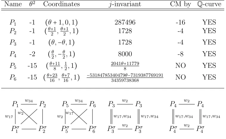
Table 8.1. X0(34)
Genus: 3
Model: x3z−x2y2−3x2z2+2xz3+3xy2z−3xyz2+4xz3−y4+4y3z−6x2z2+4yz3−2z4
J0(34)(Q) =C≅Z/4Z×Z/12Z
Name θ2 Coordinates j-invariant CM by
Q-curve
P1 -1 (θ+1,0,1) 287496 -16 YES
P2 -1 (θ+21,θ+21,1) 1728 -4 YES
P3 -1 (θ,−θ,1) 1728 -4 YES
P4 -2 (θ2,−θ2,1) 8000 -8 YES
P5 -15 (θ+811,21,1) 2041θ+811779 NO YES
P6 -15 (θ+1623,θ16+7,1) −5318478534047934359738368θ−7319387769191 NO YES
P1
w17
w34
P2 w2
Pσ
1 P2σ
P5
w2
w34
P6 w17
Pσ
5 P6σ
P3
w17,w34
w2
P3
w17,w34
Pσ 3
w2
Pσ 3
P4
w17,w34
w2
P4
w17,w34
Pσ 4
w2
Pσ 4
References
[1] A. Aigner,Uber die M¨oglichkeit vonx4
+y4=z4 in quadratischen K¨orpern, Jber. Deutsch. Math.-Verein. 43(1934), 226-229. 1, 1
[2] B. S. Banwait and J. Cremona, Tetrahedral elliptic curves and the local-to-global principle for isogenies, Algebra & Number Theory8(2014), 1201–1229. 3
[3] F. Bars,Bielliptic modular curves, J. Number Theory76(1999), no. 1, 154–165. 1
[4] W. Bosma, J. Cannon and C. Playoust, The Magma Algebra System I: The User Language, J. Symb. Comp.24(1997), 235–265. (See alsohttp://magma.maths.usyd.edu.au/magma/) 1
[5] P. Bruin and F. Najman, Hyperelliptic modular curvesX0(n)and isogenies of elliptic curves over
Table 8.2. X0(38)
Genus: 4
Model:x1x3−x22−x2x4−x23−x3x4−x24,
x21x4+x1x24−x32+3x22x3+2x22x4−3x2x23−4x2x3x4−2x2x24+x33+2x23x4+2x3x24+x34
J0(38)(Q) =C≅Z/3Z×Z/45Z
Name θ2 Coordinates j-Invariant CM by
Q-curve
P1 -3 (θ+21,0,θ−21,1) 0 -3 YES
P2 -3 (0,−θ2+1,0,1) 54000 -12 YES
P3 -2 (θ+31,−θ3+1,θ−31,1) 8000 -8 YES
P1
w19
w2
P2 w38
Pσ
1 P2σ
P3
w2,w38
w19
P3
Pσ 3
w2
Pσ 3
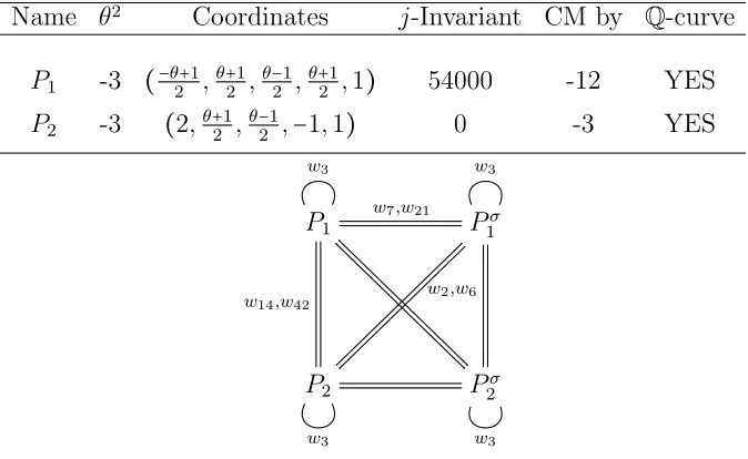
Table 8.3. X0(42) Genus :5
Model: x1x3−x22+x3x4,
x1x5−x2x5−x23+x4x5−x25,
x1x4−x2x3+x2x4−x23+x3x4+x3x5−x24−2x4x5
C≅Z/2Z×Z/2Z×Z/12Z×Z/48ZandJ0(42)(Q)/C≅0 orZ/2Z
Name θ2 Coordinates j-Invariant CM by
Q-curve
P1 -3 (−θ2+1,θ+21,θ−21,θ+21,1) 54000 -12 YES
P2 -3 (2,θ+21,θ−21,−1,1) 0 -3 YES
P1 w3
w7,w21
w14,w42
w2,w6
Pσ 1 w3
P2
w3
Pσ 2
Table 8.4. X0(44)
Genus: 4
Model: x21x4−x23+x23x4−2x34, x1x3−x22+2x2x4−3x24
J0(44)(Q) =C≅Z/5Z×Z/5Z×Z/15Z
Name θ2 Coordinates j-invariant CM by
Q-curve
P1 -7 (−θ2+1,θ+21,1,1) -3375 -7 YES
P2 -7 (θ−21,θ+21,−1,1) 16581375 -28 NO
P3 -7 (1,−θ2+1,θ+21,1) 16581375 -28 NO
P4 -7 (−1,θ+21,θ−21,1) -3375 -7 YES
P5 -7 (θ−2,−2,−θ−2,1) -3375 -7 NO
P6 -7 (−θ+2,−2, θ+2,1) -3375 -7 NO
P1
w44
w11
P4 w4
Pσ
1 P4σ
P2
w44
w11
Pσ 3 w4
P5 P6σ
Pσ 2
w44
w11
P3 w4
Pσ
[image:18.612.89.514.133.719.2]5 P6
Table 8.5. X0(45) Genus: 3
Model: x3z−x2y2+xyz2−y3z−5z4
J0(45)(Q) =C ≅Z/2Z×Z/4Z×Z/8Z
Name θ2 Coordinates j-invariant CM by
Q-curve
P1 -11 (θ−21,1,1) -32768 -11 YES
P2 -11 (−1,−θ2+1,1) -32768 -11 YES
P3 13 (2,−θ2−5,1) 1250637664527933θ64−4509238226399579 NO YES
P4 13 (−θ2+5,−2,1) 461373θ−41664219 NO YES
P5 -39 (θ+813,−θ4−5,1) 27341062251024θ+43419758443 NO YES
P6 -39 (θ+45,−θ8−13,1) −6035506678349769570368744177664θ−1556546639145161477 NO YES
P1
w45
w5
P2 w9
Pσ
1 P2σ
P3
w9
w45
P4 w5
Pσ
3 P4σ
P5
w9
w5
P6 w45
Pσ
Table 8.6. X0(51) Genus: 5
Model: x1x3−x22+x2x4−x23−x3x5−x24,
x1x4−x2x3−x23−x4x5,
x1x5−x2x4−2x23+x3x5+x24−2x4x5
J0(51)(Q) =C≅Z/8Z×Z/48Z
Name θ2 Coordinates j-invariant CM by
Q-curve
P1 -2 (0, θ/2, θ/2,1,1) 8000 -8 YES
P2 -2 (−θ9+1,2θ9−1,2θ9−1,θ+94,1) 8000 -8 NO
P3 17 (θ+25,−θ4−3,θ+43,0,1) −671956992θ−2770550784 -51 NO
P1
w51
w17
P2 w3
Pσ
1 P2σ
P3 w51
w3,w17
Pσ 3 w51
Table 8.7. X0(52) Genus: 5
Model: x1x3−x22−x23−x24,
x1x4−x2x3+x2x5−x4x5,
x1x5−x2x4−2x23+x3x5−x25
J0(52)(Q) =C ≅Z/21Z×Z/42Z
Name θ2 Coordinates j-invariant CM by
Q-curve
P1 -1 (θ+1,1,0, θ,1) 287496 -16 YES
P2 -1 (−θ2+1,0,−θ2+1,0,1) 287496 -16 YES
P3 -1 (θ+1,−1,0,−θ,1) 1728 -4 YES
P4 -3 (0,−1,θ+21,θ−21,1) 54000 -12 YES
P5 -3 (0,1,θ+21,−θ2+1,1) 54000 -12 YES
P1 w4
w13,w52
Pσ 1 w4
P2
w13
w4
P3 w52
Pσ
2 P3σ
P4
w52
w4
P5 w13
Pσ
[image:19.612.145.469.498.701.2]Table 8.8. X0(54)
Genus: 4
Model: x21x3−x1x23−x32+x22x4−3x2x24+x33+3x34,
x1x4−x2x3+x3x4
J0(54)(Q) =C≅Z/3Z×Z/3Z×Z/9Z
Name θ2 Coordinates j-Invariant CM by
Q-curve P1 -2 (−2, θ+1, θ,1) 8000 -8 YES
P1 w2
w27,w54
Pσ 1 w2
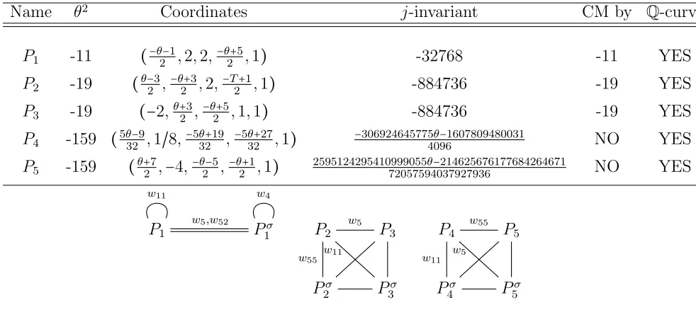
Table 8.9. X0(55)
Genus: 5
Model: x1x3−x22+x2x4−x2x5−x23+3x3x4+x3x5−2x24−4x25,
x1x4−x2x3+2x2x4−2x2x5−2x23+4x3x4+5x3x5−2x24−4x4x5−3x25,
x1x5−2x2x5−x23+2x3x4+x3x5−x24
C≅Z/10Z×Z/20Z and J0(55)(Q)/C≅0,Z/2Z or(Z/2Z)2
Name θ2 Coordinates j-invariant CM by
Q-curve
P1 -11 (−θ2−1,2,2,−θ2+5,1) -32768 -11 YES
P2 -19 (θ−23,−θ2+3,2,−T2+1,1) -884736 -19 YES
P3 -19 (−2,θ+23,−θ2+5,1,1) -884736 -19 YES
P4 -159 (532θ−9,1/8,−5θ32+19,−5θ32+27,1) −3069246457754096θ−1607809480031 NO YES
P5 -159 (θ+27,−4,−θ2−5,−θ2+1,1) 259512429541099905572057594037927936θ−214625676177684264671 NO YES
P1 w11
w5,w52
Pσ 1 w4
P2
w55
w5
P3 w11
Pσ
2 P3σ
P4
w11
w55
P5 w5
Pσ
[image:20.612.70.561.448.672.2]Table 8.10. X0(56)
Genus: 5
Model: x1x3−x22−x23+x3x5−3x24,
x1x4−x2x3+x2x5−x3x4,
x1x5−x2x4−x23+2x3x5−x24−x25
J0(56)(Q) =C≅Z/2Z×Z/6Z×Z/6Z×Z/24Z
Name θ2 Coordinates j-invariant CM by Q-curve
P1 -7 (−1,3θ8+7,−θ4+3,θ−83,1) -3375 -7 NO
P2 -7 (−1,−θ2+1,θ+21,−1,1) 16581375 -28 NO
P3 -7 (−1,−38θ−7,−θ4+3,−θ8+3,1) 16581375 -28 YES
P4 -7 (−1,θ−21,θ+21,1,1) -3375 -7 YES
P1 w7
w8,w56
Pσ 2 w7
P2 w7
w8,w56
Pσ 1 w7
P3 w7
w8,w56
Pσ 3 w7
P4 w7
w8,w56
Pσ 4 w7
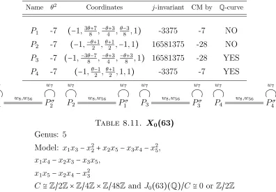
Table 8.11. X0(63) Genus: 5
Model: x1x3−x22+x2x5−x3x4−x25,
x1x4−x2x3−x3x5,
x1x5−x2x4−x23
C≅Z/2Z×Z/4Z×Z/48Z and J0(63)(Q)/C≅0 or Z/2Z
Name θ2 Coordinates j-invariant CM by
Q-curve
P1 -3 (−θ2+1,−θ2−1,θ−21,θ−21,1) 0 -3 YES
P2 -3 (θ+21,−θ2−1,1,−θ2−1,1) -12288000 -27 YES
P3 -3 (−1,θ−21,θ−21,1,1) -12288000 -27 YES
P4 -3 (0,−θ2+1,0,0,1) -12288000 -27 YES
P1
w7
w63
P4 w9
Pσ
1 P4σ
P2
w63
w7
P3 w9
Pσ
[image:21.612.137.477.521.701.2]Table 8.12. X0(64) Genus: 3
Model: x3z+4xz3−y4
J0(64)(Q) =C ≅Z/2Z×Z/4Z×Z/4Z
Name θ2 Coordinates j-invariant CM by
Q-curve P1 -7 (−θ−1,−2,1) -3375 -7 NO
P2 -7 (−θ−1,2,1) 16581375 -28 YES
P3 -7 (−θ2−1,θ+21,1) -3375 -7 YES
P4 -7 (θ−21,θ−21,1) 16581375 -28 NO
P1 w64
Pσ 4 P2
w64
Pσ 2 P3
w64
[image:22.612.93.528.130.708.2]Pσ 3
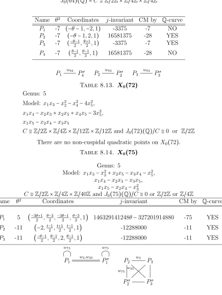
Table 8.13. X0(72) Genus: 5
Model: x1x3−x22−x 2 4−4x
2 5,
x1x4−x2x3+x2x5+x4x5−3x25,
x1x5−x2x4−x3x5
C≅Z/2Z×Z/4Z×Z/12Z×Z/12Z and J0(72)(Q)/C≅0 or Z/2Z
There are no non-cuspidal quadratic points onX0(72).
Table 8.14. X0(75)
Genus: 5
Model: x1x3−x22+x2x5−x3x4−x25,
x1x4−x2x3−x3x5,
x1x5−x2x4−x23
C≅Z/2Z×Z/4Z×Z/40Z and J0(75)(Q)/C≅0 or Z/2Z orZ/4Z
Name θ2 Coordinates j-invariant CM by
Q-curve
P1 5 (−32θ+1,θ−23,−3θ2−1,θ−23,1) 146329141248θ−327201914880 -75 YES
P2 -11 (−2,t−21,t+21,t−21,1) -12288000 -11 YES
P3 -11 (−θ2−1,θ2−1,2,θ−21,1) -12288000 -11 YES
P1 w75
w3,w25
Pσ 1 w75
P2
w75
w3
P3 w25
Pσ
Table 8.15. X0(81)
Genus: 4
Model: x21x4−x1x24−x32−3x33+x34,
x1x3−x22−2x3x4
J0(81)(Q) =C≅Z/3Z×Z/9Z
Name θ2 Coordinates j-Invariant CM by
Q-curve P1 -2 (−2θ,θ2−1,θ2, ,1) 8000 -8 YES
P2 -11 (−θ2−1,−θ2+1,1,1) -32768 -11 YES
P1 w81
Pσ 1 P2
w81
Pσ 2
[6] N. Bruin, B. Poonen and M. Stoll,Generalized explicit descent and its application to curves of genus3, Forum Math. Sigma4(2016), e6, 80 pp. 5.5
[7] J. J. Cannon and D. F. Holt,Automorphism group computation and isomorphism testing in finite groups, Journal of Symbolic Computation35(2003), 241–267. 4
[8] J. E. Cremona,Algorithms for Modular Elliptic Curves, Cambridge University Press, 1992. 3
[9] M. Derickx, Torsion points on elliptic curves over number fields of small degree, PhD thesis, Leiden University, 2016.
[10] M. Derickx, S. Kamienny, W. Stein and M. Stoll, Torsion Points on Elliptic Curves over Number Fields of Small Degree,arXiv:1707.00364v1. 1
[11] F. Diamond and J. Shurman,A First Course on Modular Forms, GTM228, Springer, 2005. 2, 3 [12] V. G. Drinfel’d,Two theorems on modular curves (Russian), Funkcional. Anal. i Priloˇzen. 7 (1973), no.
2, 83–84. 1
[13] S. D. Galbraith,Equations for Modular Curves, DPhil thesis, University of Oxford, 1996. 2, 3
[14] B. Gross and J. Harris,Real algebraic curves, Ann. Sci. ´Ecole Norm. Sup. (4)14(1981), no. 2, 157–182. 5.3, 5.3
[15] N. Freitas, B. V. Le Hung and S. Siksek, Elliptic Curves over Real Quadratic Fields are Modular, Inventiones Mathematicae201(2015), 159–206. 1, 3
[16] N. Freitas, S. Siksek, Fermat’s last theorem over some small real quadratic fields, Algebra Number Theory9(2015), no. 4, 875-895. 1
[17] J. Harris and J. Silverman, Bielliptic curves and symmetric products, Proc. Amer. Math. Soc. 112 (1991), no. 2, 347–356. 1
[18] F. Hess, Computing Riemann–Roch spaces in algebraic function fields and related topics, J. Symbolic Comput.33(2002), no. 4, 425–445. 5.1
[19] S. Kamienny, Torsion points on elliptic curves and q-coefficients of modular forms, Invent. Math.,109 (1992), no. 2 221-229 1
[20] N. M. Katz, Galois properties of torsion points on abelian varieties, Invent. Math. 62 (1981), no. 3, 481–502. 5.1, 6
[21] V. A. Kolyvagin and D. Yu. Logach¨ev,Finiteness of the Shafarevich–Tate group and the group of rational points for some modular abelian varieties(Russian), Algebra i Analiz1(1989), no. 5, 171–196; translation in Leningrad Math. J.1(1990), no. 5, 1229–1253. 2
[22] M. A. Kenku,On the modular curvesX0(125),X1(25)andX1(49), J. London Math. Soc. (2)23(1981), no. 3, 415-427. 1
[24] B. D. McKay,Practical Graph Isomorphism, Congressus Numerantium30(1981), 45–87. 5.5
[25] Ju. I. Manin,Parabolic points and zeta functions of modular curves (Russian), Izv. Akad. Nauk SSSR Ser. Mat.36(1972), 19–66. 1
[26] B. Mazur,Modular curves and the Eisenstein ideal, Inst. Hautes ´Etudes Sci. Publ. Math. No.47(1977), 33–186. 1, 1
[27] B. Mazur,Rational isogenies of prime degree, Invent. Math.44(1978), no. 2, 129–162. 1
[28] L. Merel, Bornes pour la torsion des courbes elliptiques sur les corps de nombres, Invent. Math.124 (1996), no. 1-3, 437–449. 1
[29] M. Ohta, Eisenstein ideals and the rational torsion subgroups of modular Jacobian varieties II, Tokyo J. Math.37(2014), 273–318. 1
[30] A. P. Ogg,Hyperelliptic modular curves, Bulletin de la S. M. F.102(1974), 449–462. 2 [31] E. Ozman and S. Siksek,Quadratic Points on Modular Curves II, in progress 1
[32] P. Parent, Bornes effectives pour la torsion des courbes elliptiques sur les corps de nombres, J. Reine Angew. Math.,506(1999) 85-116. 1
[33] P. Parent, Torsion des courbes elliptiques sur les corps cubiques, Ann. Inst. Fourier (Grenoble), 50 (2000), no. 3, 723-749. 1
[34] B. Poonen and E. F. Schaefer, Explicit descent for Jacobians of cyclic covers of the projective line, J. Reine Angew. Math.488(1997), 141–188. 5.2
[35] Y. Ren,Rational torsion subgroups of modular Jacobian varieties, Journal of Number Theory, to appear. 1, 1
[36] S. Siksek,Chabauty for symmetric powers of curves, Algebra & Number Theory3(2009), no. 2, 209–236. 1
[37] A. Snowden,Real components of modular curves,arXiv:1108.3131. 5.3
[38] W. A. Stein,Explicit approaches to modular abelian varieties, University of California at Berkeley PhD thesis, 2000. 2
[39] W. A. Stein,Modular Forms: A Computational Approach, American Mathematical Society, 2007. 2, 3 [40] M. Stoll,Implementing 2-descent for Jacobians of hyperelliptic curves, Acta Arith.98(2001), 245–277.
2
[41] H. Yoo,The index of an Eisenstein ideal and multiplicity one, Math. Z.282(2016), 1097–1116. 1
Bogazici University, Department of Mathematics, Bebek, Istanbul, 34342, Turkey E-mail address: [email protected]