Autonomous Anomaly Detection
Xiaowei Gu,
Student Member
,
IEEE
and Plamen Angelov,
Fellow
,
IEEE
Data Science Group,School of Computing and Communications, Lancaster University, Lancaster, UK E-mail: {x.gu3, p.angelov}@lancaster.ac.uk
Abstract—In this paper, a new approach for autonomous
anomaly detection is introduced within the Empirical Data Analytics (EDA) framework. This approach is fully data-driven and free from thresholds. Employing the nonparametric EDA estimators, the proposed approach can autonomously detect anomalies in an objective way based on the mutual distribution and ensemble properties of the data. The proposed approach firstly identifies the potential anomalies based on two EDA criteria, and then, partitions them into shape-free non-parametric data clouds. Finally, it identifies the anomalies in regards to each data cloud (locally). Numerical examples based on synthetic and benchmark datasets demonstrate the validity and efficiency of the proposed approach.
Keywords—autonomous anomaly detection; Empirical Data Analytics (EDA); nonparametric; data cloud.
I. INTRODUCTION
Anomaly detection is an important problem of statistical analysis [1]. Anomaly detection techniques mainly target discovering rare events [2]. In many real situations and applications, i.e. detecting criminal activities, forest fire, human body monitoring, etc., the rare cases play a key role. Anomaly detection is also closely linked to clustering process since the members of a cluster are rather routine, normal or typical [2] and, thus, data either belong to a cluster or are anomalous.
Traditional anomaly detection is based on the statistical analysis [3], [4]. It relies on a number of prior assumptions about the data generation models and requires certain degree of prior knowledge [3]. However, those prior assumptions are only true in the ideal/theoretical situations, i.e. Gaussian, independently and identically distributed data, but the prior knowledge is more often unavailable in reality.
There are some supervised anomaly detection approaches published in the recent decades [5]–[7]. Those techniques require the labels of the data samples to be known in advance, which allows the algorithms to learn in a supervised way and generate the desired output after training. The supervised approaches are usually more accurate and effective in detecting outliers compared with the statistical methods. However, in real applications, the labels of the data are usually unknown. The existing unsupervised anomaly detection approaches [8]–[10], however, require a number of user inputs to be pre-defined, i.e. threshold, error tolerance, number of
nearest neighbors, etc. Selection of the proper user inputs requires good prior knowledge; otherwise, the performance of those approaches is affected.
Empirical data analytics (EDA) framework [2], [11]–[13] is a recently introduced nonparametric, fully data-driven methodology for data analysis. EDA is entirely based on the empirically observed data and their ensemble properties without any prior assumptions. It is a powerful extension of the traditional probability theory and statistical learning.
In this paper, the nonparametric EDA estimators, cumulative proximity, unimodal density and multimodal density [2], [11]–[13] are employed to identify the potential anomalies from the empirically observed data at the first stage of the process. Then, we use those potential anomalies to form shape-free data clouds using a newly introduced nonparametric data partitioning approach [14]. The concept of the data cloud was introduced in [15] as the collection of data samples based on their mutual distribution and ensemble properties. Finally, the local anomalies are identified in regards to the data clouds. Numerical examples demonstrate that the proposed approach can autonomously and objectively detect both individual and collective anomalies (remote, small clouds) and also global anomalies as well as anomalies that are centrally located.
The remainder of this paper is organized as follows. Section II briefly describes the theoretical basis. The procedure of the proposed approach is introduced in section III in detail. Section IV presents numerical examples and the discussion is given in section V. This paper is concluded by section VI.
II. THEORETICAL BASIS
In this section, we will describe the EDA estimators [2], [11]–[13] employed by the proposed approach:
i) cumulative proximity [2], [11].
ii) unimodal density [12], [13];
iii) multimodal density [12], [13].
First of all, let us consider the real Hilbert space d
R and assume a particular dataset denoted as:
1, 2,...,
dK R
x x x ,
where xi denotes the ith data sample and K is the total
number of data samples. Within this dataset, often there are
more than one data sample which have the same value, namely | i j
i j
x x . The set of unique data samples is denoted as:
1, 2,...,
d L R
u u u and the corresponding frequencies are
defined as:
f f1, 2,...,fL
, where1 L i i f K
, LK. In thispaper, the Euclidean distance is used for derivation clarity, however other types of distances can be considered as well.
A. Cumulative Proximity
The cumulative proximity of a particular data sample xi is defined as the sum of square distances fromxi to all the existing data samples in d
R [2], [11]:
2
2 2
1
K
i i j i
j
K X
x x x x (1)
where
21
d l l
i j i j
l
x x
x x is the Euclidean distance
between xi and xj;
1 1 K
i i
K
x
; 21 1 K i i X K
x .B. Unimodal Density
Unimodal density within EDA framework [12], [13] is an important measure centered at the main mode of the data distribution defined as the inverse of normalized cumulative proximity:
2 1 1 1 2 2 2 1 1 2 2 1 K K K k j k k j UM k i K i i i j j D K K X
x x x x x xx x
(2)
where the coefficient 2 is used in the numerator of DUM
xidue to the fact that each distance is counted twice in the sum of cumulative proximities of all the data samples and the following equality holds [13]:
2 2
2
1 1 1
2
K K K
k k j
k k j
K X
x
x x (3)From equation (2) one can see that the unimodal density is in the form of a Cauchy function when using Euclidean distance. However, this is not a prior assumption about the type of the distribution and only holds for Euclidean type of distance.
C. Multimodal Density
The multimodal density [12], [13] of a unique data sample is defined as a weighted unimodal density by the corresponding frequency. It has the ability of disclosing the local modes of the data distribution directly from the data without using iterative searching algorithms [12], [13]. The multimodal density at a particular unique data sample ui is expressed as:
22 1
MM UM i
i i i
i
f
D f D
X u u u (4)
Consider the original dataset
x x1, 2,...,xK
, for
j k i jk
x x u , the following equation holds:
MM MM UM
j k i i
D x D x f D u (5) D. Chebyshev Inequality
It is well-known that, the Chebyshev inequality [16] is very important for detecting anomalies empirically [2], [17], [18]. Using the Euclidean distance, the inequality has the following form:
2 2 2
2 1 P n n
x (6)
where 2 X 2. The Chebyshev inequality describes the probability data samples to be more than n distance away from the mean value,
. As a corollary, if n3, the maximum probability of x to be at least 3
away from
isno more than 1
9. In other words, on average, out of 9 data samples, one may be anomalous, but no more than 1 (at most 1).
III. THE PROPOSED METHOD
In this section, we will describe the proposed autonomous and data-driven anomaly detection approach in detail. Its procedure consists of 3 stages as follows.
A. Identifying Potential Anomalies
In the first stage, the global mean and average scalar product,
and X of
x x1, 2,...,xK
are calculated. Then,the multimodal densities, MM
D , at
u u1, 2,...,uL
are obtainedusing equation (4). By extending the multimodal densities at
u u1, 2,...,uL
to the original dataset
x x1, 2,...,xK
, themultimodal densities at
x x1, 2,...,xK
are obtained as
MM
D x . After ranking
DMM
x
in ascending order, weselect the first half of 2 1
n of the data samples with the smallest MM
D being the first half of the potential anomaly collection (see equation (6)), denoted as
1
PA
first stage of sub-selection of potential anomalies (an upper limit according to equation (6)).
As the multimodal density is less sensitive to the degree of sparsity of local data distribution, an additional criterion is necessary for detecting the isolated data samples. We consider the weighted local unimodal density as the second criterion for identifying potential anomalies.
Firstly, the average square Euclidean distance between each pair of data samples within
x x1, 2,...,xK
is obtained from the following equation:
2
2 1 2 2 K k k d X K
x (7)
For each unique data sampleui, one can obtain a
hyper-sphere defined by the center ui and the radius of 2 d
as its
local influence area. All other unique data samples within this hyper-sphere are categorized as ui’s unique neighbors:
2 i i d IFTHEN is neighbouring to
u u
u u
(8)
We denote all the nearby data samples satisfying the
condition (8) as the set
u iL with a cardinality Ni. Based on
Li
u , the local unimodal density at ui is calculated as:
22 1 1 L i L i i L L i i D U u u
(9)where iL denotes the mean of
L iu and UiL denotes their
average scalar product.
By taking both, the sparsity of data distribution of the local area around ui and the frequency of occurrence into consideration, the local unimodal density at ui is weighed by its frequency and the amount of its unique neighbors as:
i 1
WL L
i i i
N
D f D
L
u u (10)
where the coefficient
Ni 1
L
is for ensuring the value of
WL i
D u to be linearly and inversely correlated to the degree of sparsity of the data distribution. By expanding the weighted local unimodal densities, WL
D , at
u u1, 2,...,uL
to the original dataset
x x1, 2,...,xK
accordingly, the set
DWL
x
is obtained. After re-ranking the
DWL
x
in the ascendingorder, the first half of 2 1
n of the data samples with smallest
WL
D are selected as the second half of the potential anomaly collection, denoted as
2
PA
x .
Finally, by combining
1PA
x and
2
PA
x (together 2 1
n or less of the data), we obtain the whole set of potential
anomalies,
x PA, which forms the upper limit of possible anomalies according to equation (6).B. Forming Data Clouds
In this subsection, we will check if the identified potential anomalies can form data clouds. The main procedure of the recently introduced free-shape data partitioning algorithm within the EDA framework is summarized as follows [14].
Free-shape data partitioning algorithm
i. Calculate the multimodal density MM
D at
x PAusing equation (4);ii. Find the potential anomaly x1PA with the maximum
multimodal density DMM
x1PA ;iii. Remove x1PA from
PAx and send x1PA to
PA descendingx ;
iv. xR x1PA;
v. While
x PA1. i i 1
2. Find the potential anomaly, denoted as PA i
x that is nearest to R
x ;
3. Remove xiPA from
x PA and send xiPA to
PA descendingx ;
4. R PA
i
x x ;
vi. End While
vii. Filter
PAdescending
x using equation (11) and obtain data samples at which DMM hold its local maxima, denoted as
x LM:
sgn 1MM PA MM PA
j j
IF D x D x
1
sgn DMM xPAj DMM xPAj 1
sgn 1 1
MM PA MM PA
j j
AND D x D x
MM PA
j
THEN D has one of its local maxima at x (11)
where
1 0
sgn 0 0
1 0 x x x x .
1. Form data clouds from
x PA by using
x LM as focal points:
arg min ;
LM
PA
i i i
cloud label
y x
x y x x (12)
2. Obtain the centers (means),
and the average scalar products,
P of the data clouds;3. Calculate the multimodal densities at the cloud centers:
2
2 ; 1 MM i i i i S D X
c c c
c
(13)
where ciis the center of the ith data cloud and Si is the (number of members).
4. Find the neighbors of each center using the following equation:
1 i j j i IF dTHEN is neighboring
c c
c c
(14)
wherec ci, j
c ;i j; d is the average Euclidean distance between two centers; is the standard deviation of the distances.5. Filter out the local maxima
c LM satisfying the following condition:
max Neighbour,
MM MM MM
i i i
i
IF D D D
THEN is one of the local maxima
c c c
c
(15)
where
MM
Neighbour iD c denotes the set of
multimodal densities at the centers neighboring ci.
6.
x LM
c LM ; x. End Whilexi. Form data clouds from
x PA using
x LM.After the data clouds are formed from
x PA based on the free-shape data partitioning algorithm [14], the proposed anomaly detection algorithm enters the last stage.C. Identifying Local Anomalies in regards to the Identified Data Clouds
In the final stage, we check if the potential anomalies are isolated or form minor data cloud(s) between themselves. All
the data clouds formed from
x PA are being checked and anomalies are identified and declared/confirmed.Let us assume that there are N data clouds formed from
PAx denoted as Ci,i1, 2,...,N.
We declare all potential anomalies as actual anomalies unless they form data clouds between themselves with a support above the average:
i average
i
IF S S
THEN is formed by anomalies
C
(16)
where the average support of those data clouds is calculated as
1 1 N average i i S S N
.IV. CASE STUDIES
In this section, a number of numerical examples based on synthetic and benchmark datasets conducted to evaluate the performance of the proposed algorithm are summarized. We have to stress that the proposed anomaly detection approach is unsupervised and autonomous; the anomalies are identified merely based on the empirically observed data samples. Therefore, in the numerical experiments presented in this paper, the labels of the data samples are unknown.
A. Synthetic Dataset
The first numerical example is based on a synthetic Gaussian dataset, which contains 720 samples with 2 attributes. There is 1 larger cluster and 2 smaller ones grouping 700 data samples between them. In addition, 4 collective anomalous sets formed by 18 samples as well as 2 single anomalies were identified. The models of the three major clusters extracted from the data ( , ,S) are as follows (in the form of model, x~N
,
and support,S):Major cluster 1: ~ 0 3 , 0.09 0 0 0.09
x N , 400 samples;
Major cluster 2: ~ 2.5 3 , 0.16 0 0 0.16
x N , 150 samples;
Major cluster 3: ~ 2.5 0 , 0.16 0 0 0.16
x N , 150 samples;
The models of the 4 collectives anomalous sets are:
Anomalous set 1: ~ 0 1 , 0.09 0 0 0.09
x N , 5 samples;
Anomalous set 2: ~ 4.5 0 , 0.09 0 0 0.09
x N , 4 samples;
Anomalous set 3: ~ 4.5 4 , 0.01 0 0 0.01
x N , 5 samples;
Anomalous set 4: ~ 1 1 , 0.01 0 0 0.01
x N , 4 samples.
and the two single anomalies are [2 5] and [1.5 2].
Fig. 1. Visualization of the synthetic dataset
Fig. 2. Identified potential anomalies (Stage 1)
Fig. 3. Checking the potential anomalies for possible data clouds between them (Stage 2)
Fig. 4. Identified anomalies (Stage3)
Fig. 5. The identified anomalies by the ODRW algorithm
Using the proposed approach, 61 potential anomalies identified in the first stage are depicted in Fig. 2 (the green
dots). In stage 2, 10 data clouds are formed from the potential anomalies as presented in Fig. 3, where the dots with the different colors are the data samples from different data clouds. There are 31 anomalies identified in the final stage of the proposed approach as shown in Fig. 4 (red dots).
Figs. 1-4 show that, the proposed approach successfully identified all the anomalies in this dataset, because both, the mutual distribution and the ensemble properties of the data samples have been considered.
For further evaluation of our proposal, two well-known traditional approaches are used for comparison:
i) The well-known “ 3” approach [2], [17], [18];
ii) Outlier detection using random walks (ODRW) approach [9].
It has to be stressed that the “ 3” approach is based on the global mean and global standard deviation. The outlier detection using random walks approach requires three parameters to be pre-defined: i) error tolerance, ; ii) similarity threshold, Tand iii) number of anomalies, N0. In this numerical example, the three parameters are set to:
6 10
, T 0.9 and N0 31 to make the results comparable.
The global mean and the standard deviation of the dataset are
1.1077 2.3263
and
1.3401 1.3228
, and the “ 3” approach failed to detect any anomalies.The result using the ODRW approach is shown in Fig. 5, where the red dots are the identified anomalies. As we can see, this approach ignored the majority of the anomalies (circled within the yellow ellipsoids).
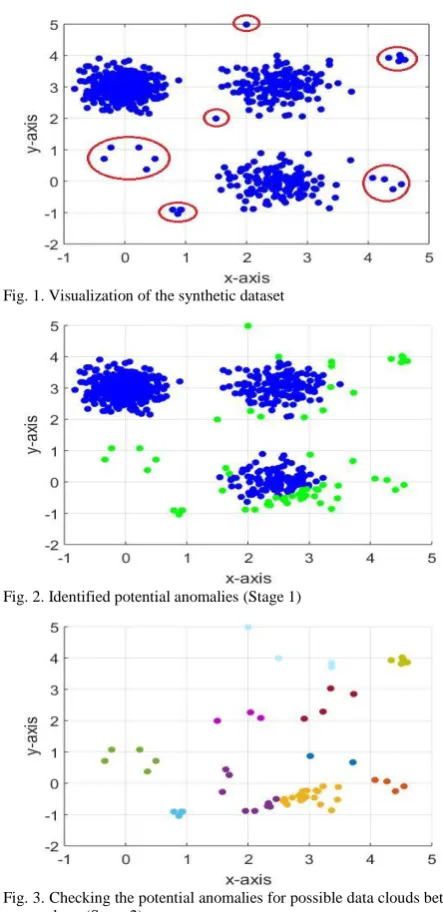
B. User Knowledge Modelling Dataset [19]
We use the real dataset about the students’ knowledge status about the subject of Electrical DC Machines published in [19] as the second example. This dataset contains 403 samples that has 5 attributes:
i) STG: The degree of study time for goal object materials;
[image:5.595.313.530.63.201.2]TABLE I. DETECTED ANOMALIES
# ID Values Label
[image:6.595.309.555.59.283.2]1 [0.0000 0.0000 0.0000 0.0000 0.0000] Very Low 2 [0.0800 0.0800 0.1000 0.2400 0.9000] High 5 [0.0800 0.0800 0.0800 0.9800 0.2400] Low 17 [0.0500 0.0700 0.7000 0.0100 0.0500] Very Low 187 [0.4950 0.8200 0.6700 0.0100 0.9300] High 210 [0.8500 0.0500 0.9100 0.8000 0.6800] High 222 [0.7700 0.2670 0.5900 0.7800 0.2800] Middle 242 [0.7100 0.4600 0.9500 0.7800 0.8600] High 399 [0.9000 0.7800 0.6200 0.3200 0.8900] High 403 [0.6800 0.6400 0.7900 0.9700 0.2400] Middle
Fig. 6. Visualization of anomalies per attribute
TABLE II. THE PERFORMANCE COMPARISON
Approach NA P FA R t
3σ 1 100% 0.00% 98.55% 0.00 ODRW 10 50.00% 1.50% 92.75% 0.27 The proposed 10 90.00% 0.30% 86.96% 0.09
iii) STR: The degree of study time of user for related objects with goal object;
iv) LPR: The exam performance of user for related objects with goal object;
v) PEG: The exam performance of user for goal objects.
and 1 label - UNS: The knowledge level of user. There are four levels of the user knowledge, i) High (130 samples), ii) Middle (122 samples), iii) Low (129 samples) and iv) Very Low (50 samples), the mean values of the data samples of the four levels are:
i) High:
high
0.4069 0.4305 0.5098 0.5429 0.7998
;ii) Middle:
middle
0.3746 0.3672 0.4911 0.3857 0.53 14
;iii) Low:
low
0.3268 0.3228 0 .4250 0.4 493 0.2536
;iv) Very Low: very
0.2592 0.2619 0 .3540 0.2688 0.09 58
low
.
The existing anomalies in four classes are listed by their IDs as follows:
i) High: 2, 10, 14, 34, 182, 187, 190, 210, 230, 246, 258, 313, 317, 318, 378, 379, 384, 391, 399, 400.
ii) Middle: 4, 13, 50, 57, 62, 65, 124, 130, 162, 207, 208, 211, 212, 214, 222, 223, 245, 250, 257, 272, 286, 362, 372, 373, 403.
iii) Low: 3, 5, 18, 53, 61, 128, 129, 131, 198, 204, 244, 319, 374, 395, 401.
iv) Very Low: 1, 17, 117, 197, 209, 288, 310, 312, 314.
Using the proposed approach, we identified 10 anomalies as tabulated in Table I. The visualization of the anomalies per attribute is depicted in Fig. 6. We have to stress that the labels (Table I) of the data are not used in the anomaly detection and we just use them for posterior comparison.
From Table I, we can see, the detected anomalies have significantly lower or higher values compared with other members of the classes to which they may belong. 9 out of the identified 10 anomalies are in the anomaly lists above.
The “ 3 ” approach and the ODRW approach are again used for comparison. In this numerical example, the three
parameters of the ODRW approach are set as:
106, 0.9T and N0 10. The details of the comparison are tabulated in Table II. The performance evaluation is based on the following four measures [9]:
i) Number of identified anomalies (NA):NATPFP; ii) Precision (P): the rate of true anomalies in the detected
anomalies,
T F
TP P
P P
;
iii) False alarm rate (FA): the rate of the true negatives in
the identified anomalies, FA FP
TN FP
;
iv) Recall rate (R): the rate of true anomalies the
algorithms missed, R FN
FN TP
;
v) Execution time (t): in seconds.
where TPand FPare the numbers of true and false positives; TNand FN are the numbers of true and false negatives.
The “ 3” approach only identified 1 anomaly, which is:
230 0.9900 0.4900 0.0700 0.7000 0.6900
x
TABLE III. THE PERFORMANCE COMPARISON
Approach NA P FA R t
3σ 141 30.05% 6.57 % 60.19% 0.01 ODRW 36 0.00% 2.41% 100.00% 31.14 The proposed 36 63.89% 0.87% 78.70% 0.24
TABLE IV. THE PERFORMANCE COMPARISON
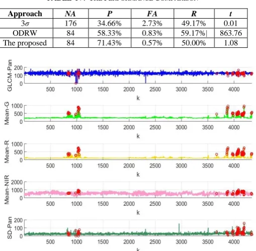
Approach NA P FA R t
3σ 176 34.66% 2.73% 49.17% 0.01 ODRW 84 58.33% 0.83% 59.17%| 863.76 The proposed 84 71.43% 0.57% 50.00% 1.08
Fig. 7. Visualization of anomalies per attribute
C. Wine Quality Dataset [20]
This dataset is related to the quality of red Portuguese “Vinho Verde” wine. This dataset has 1599 data samples with 11 attributes: i) fixed acidity, ii) volatile acidity, iii) citric acid, iv) residual sugar, v) chlorides , vi) free Sulphur dioxide, vii) total Sulphur dioxide, viii) density, ix) pH, x) Sulphates, xi) alcohol and 1 label: the score of quality from 3 to 8.
This dataset is not balanced as there are much more normal wines than excellent or poor ones. There are 10 samples with score 3, 53 samples with score 4, 681 samples with score 5, 638 samples with score 6, 199 samples with score 7 and 18 samples with score 8.
The number of existing anomalies in each class are listed as follows: i) Score 3: 1; ii) Score 4: 3; iii) Score 5: 50; iv) Score 6: 42; v) Score 7: 9; vi) Score 8: 3. In total, there are 108 anomalies.
The results of the three anomaly detection approaches based on the wine quality dataset are tabulated in Table III. In this example, the three parameters of the ODRW approach are set as:
106, T 0.9 and N0 36.D. Wilt Dataset [21]
This dataset comes from a remote sensing study involving detecting diseased trees in Quickbird imagery. There are two classes in the dataset: i) “diseased trees” class (74 samples) and ii) “other land cover” class (4265 samples) [21]. Each sample has 5 attributes:
i) GLCM-Pan: GLCM mean texture (Pan band) ;
ii) Mean-G: mean green value;
iii) Mean-R: mean red value;
iv) Mean-NIR: mean NIR value;
v) SD-Pan: standard deviation (Pan band).
There are 120 anomalies with the label “other land cover” and no anomaly in the “diseased trees” class.
Using the proposed approach, 84 anomalies are detected in this dataset. The identified anomalies are visualized in Fig. 7 per attribute.
Similarly, the performance of the proposed approach is compared with the two algorithms used in section IV. A. The results are tabulated in Table IV. In this numerical example, the three parameters of the ODRW approach are set as:
6 10
, T 0.9 and0 84
N .
V. DISCUSSION
From Tables II, III and IV one can see that the proposed approach is able to detect the anomalies with higher precision and lower false alarm rate compared with the“ 3” approach and the ODRW approach.
The “ 3” approach is the fastest due to its simplicity. However, the performance of the “ 3” approach is decided by the structure of the data as it focuses only on the samples exceeding the global 3 range around the mean. However, when the dataset is very complex i.e. contains a large number of clusters, or the anomalies are close to the global mean, “ 3” approach fails to detect all outliers.
In contrast, the proposed approach can identify the anomalies based on the ensemble properties of the data in a fully unsupervised and autonomous way. It takes not only the mutual distribution of the data within the data space, but also the frequencies of occurrences into consideration. It provides a more objective way for anomaly detection. More importantly, its performance is not influenced by the structure of the dataset and is equally effective in detecting collective as well as individual anomalies.
VI. CONCLUSION
In this paper, a fully autonomous anomaly detection approach within EDA framework is introduced. This approach is entirely data-driven and unsupervised. It employs the non-parametric EDA estimators to disclose the underlying data pattern and identify the potential anomalies based on the mutual distribution and ensemble properties of the data. By analyzing the data set/stream in two stages:
[image:7.595.37.284.82.128.2] [image:7.595.38.293.436.685.2]ii) Identifying and declaring local anomalies after forming possible data clouds from the potential anomalies;
the proposed approach offers a deeper analysis and more precise result.
Numerical examples demonstrate the excellent performance of the proposed approach as well as its high computational efficiency. The proposed approach is highly suitable to real situations where prior knowledge of the data is unavailable. It can be an effective pre-processing tool as well.
REFERENCES
[1] V. Chandola, A. Banerjee, and V. Kumar, “Anomaly detection: A survey,” ACM Comput. Surv., vol. 41, no. 3, pp. 1–6, 2009.
[2] P. P. Angelov, “Anomaly detection based on eccentricity analysis,” in
2014 IEEE Symposium Series in Computational Intelligence, IEEE Symposium on Evolving and Autonomous Learning Systems, EALS, SSCI 2014, 2014, pp. 1–8.
[3] C. M. Bishop, Pattern Recognition. New York: Springer, 2006. [4] A. Bernieri, G. Betta, and C. Liguori, “On-line fault detection and
diagnosis obtained by implementing neural algorithms on a digital signal processor,” IEEE Trans. Instrum. Meas., vol. 45, no. 5, pp. 894–899, 1996.
[5] M. M. Breunig, H.-P. Kriegel, R. T. Ng, and J. Sander, “LOF: Identifying Density-Based Local Outliers,” in Proceedings of the 2000 Acm Sigmod International Conference on Management of Data, 2000, pp. 1–12.
[6] N. Abe, B. Zadrozny, and J. Langford, “Outlier detection by active learning,” in IACM nternational Conference on Knowledge Discovery and Data Mining, 2006, pp. 504–509.
[7] S. S. Sivatha Sindhu, S. Geetha, and A. Kannan, “Decision tree based light weight intrusion detection using a wrapper approach,” Expert Syst. Appl., vol. 39, no. 1, pp. 129–141, 2012.
[8] V. Hautam and K. Ismo, “Outlier Detection Using k-Nearest Neighbour Graph,” in International Conference on Pattern Recognition, 2004, pp. 430–433.
[9] H. Moonesinghe and P. Tan, “Outlier detection using random walks,” in
Proceedings of the 18th IEEE International Conference on Tools with Artificial Intelligence (ICTAI’06), 2006, pp. 532–539.
[10] M. Salehi, C. Leckie, J. C. Bezdek, T. Vaithianathan, and X. Zhang, “Fast Memory Efficient Local Outlier Detection in Data Streams,” IEEE Trans. Knowl. Data Eng., vol. 28, no. 12, pp. 3246–3260, 2016. [11] P. Angelov, “Outside the box: an alternative data analytics framework,”
J. Autom. Mob. Robot. Intell. Syst., vol. 8, no. 2, pp. 53–59, 2014. [12] P. P. Angelov, X. Gu, J. Principe, and D. Kangin, “Empirical data
analysis - a new tool for data analytics,” in IEEE International Conference on Systems, Man, and Cybernetics, 2016, pp. 53–59. [13] P. Angelov, X. Gu, and D. Kangin, “Empirical data analytics,” Int. J.
Intell. Syst., 2016, to appear.
[14] X. Gu, P. P. Angelov, and J. Principe, “Forming data clouds: free-shape data partitioning through empirical data analysis,” Submitt. to IEEE Trans. Neural Networks Learn. Syst.
[15] P. Angelov and R. Yager, “A new type of simplified fuzzy rule-based system,” Int. J. Gen. Syst., vol. 41, no. 2, pp. 163–185, 2011.
[16] J. G. Saw, M. C. K. Yang, and T. S. E. C. Mo, “Chebyshev inequality with estimated mean and variance,” Am. Stat., vol. 38, no. 2, pp. 130– 132, 1984.
[17] D. E. Denning, “An Intrusion-Detection Model,” IEEE Trans. Softw. Eng., vol. SE-13, no. 2, pp. 222–232, 1987.
[18] C. Thomas and N. Balakrishnan, “Improvement in intrusion detection with advances in sensor fusion,” IEEE Trans. Inf. Forensics Secur., vol. 4, no. 3, pp. 542–551, 2009.
[19] “User Knowledge Modeling Dataset,”
https://archive.ics.uci.edu/ml/datasets/User+Knowledge+Modeling#. [20] “Wine Quality Dataset,”