Modeling and controller design of a 6 DOF precision positioning system

warwick.ac.uk/lib-publications

Cai, Kunhai, Tian, Yanling, Liu, Xianping, Fatikow, S., Wang, Fujun, Cui, Liangyu, Zhang, Dawei and Shirinzadeh, Bijan(2018) Modeling and controller design of a 6-DOF precision

positioning system. Mechanical Systems and Signal Processing, 104. pp.

536-555. doi:10.1016/j.ymssp.2017.11.002

Permanent WRAP URL:

http://wrap.warwick.ac.uk/94384

Copyright and reuse:

The Warwick Research Archive Portal (WRAP) makes this work by researchers of the University of Warwick available open access under the following conditions. Copyright © and all moral rights to the version of the paper presented here belong to the individual author(s) and/or other copyright owners. To the extent reasonable and practicable the material made available in WRAP has been checked for eligibility before being made available.

Copies of full items can be used for personal research or study, educational, or not-for-profit purposes without prior permission or charge. Provided that the authors, title and full bibliographic details are credited, a hyperlink and/or URL is given for the original metadata page and the content is not changed in any way.

Publisher’s statement:

© 2018, Elsevier. Licensed under the Creative Commons Attribution-NonCommercial-NoDerivatives 4.0 International http://creativecommons.org/licenses/by-nc-nd/4.0/

A note on versions:

The version presented here may differ from the published version or, version of record, if you wish to cite this item you are advised to consult the publisher’s version. Please see the ‘permanent WRAP URL’ above for details on accessing the published version and note that access may require a subscription.

Modeling and Controller Design of a 6-DOF

Precision Positioning System

Kunhai Cai1,2, Yanling Tian1*,2, Xianping Liu2, Sergej Fatikow3, Fujun Wang1, Liangyu Cui1, Dawei

Zhang1, Bijan Shirinzadeh4

1

Key Laboratory of Mechanism Theory and Equipment Design of Ministry of Education, Tianjin University, Tianjin 300072, China

2

School of Engineering, University of Warwick, Coventry CV4 7AL, UK

3

Division of Microrobotics and Control Engineering, University of Oldenburg, 26111 Oldenburg, Germany

4

Robotics and Mechatronics Research Laboratory, Department of Mechanical and Aerospace

Engineering, Monash University, Clayton, VIC 3800, Australia

Abstract: A key hurdle to meet the needs of micro/nano manipulation in some complex cases is the inadequate workspace and flexibility of the operation ends. This paper presents a 6-degree of freedom (DOF) serial-parallel precision positioning system, which consists of two compact type 3-DOF parallel mechanisms. Each parallel mechanism is driven by three piezoelectric actuators (PEAs), guided by three symmetric T-shape hinges and three elliptical flexible hinges, respectively. It can extend workspace and improve flexibility of the operation ends. The proposed system can be assembled easily, which will greatly reduce the assembly errors and improve the positioning accuracy. In addition, the kinematic and dynamic model of the 6-DOF system are established, respectively. Furthermore, in order to reduce the tracking error and improve the positioning accuracy, the Discrete-time Model Predictive Controller (DMPC) is applied as an effective control method. Meanwhile, the effectiveness of the DMCP control method is verified. Finally, the tracking experiment is performed to verify the tracking performances of the 6-DOF stage.

1. Introduction

The roles of precision positioning technology have become increasingly important in various industry fields, such as nano-imprint [1], cell operation [2], scanning probe microscopes[3], optical instruments [4], measurement systems [5,6] and micro/nano manipulations [7,8,9], a precision positioning system possesses such advantages as high positioning accuracy, fast response speed, satisfactory stability and dynamic characteristics. It mainly composed of drives, guide mechanism and operation ending three parts. The piezoelectric actuator (PEA) is the main type of actuator which is often used to actuate a positioning mechanism. Because, PEAs offer the extremely fine resolution, quick response, large force generation and small volume. In addition, the guide mechanism is a key factor in positioning system design, which will decide the motion performance and dynamic characteristics of the system. The flexure mechanism is a normal choice as they avoid many disadvantages including backlash, wear, lubrication and friction, compare with the other guide mechanisms. In the past decade, most of the existing precision positioning systems were designed and featured by one-three-DOF motions. Such as, a flexure-based mechanism for ultra-precision operation with 1-DOF, and a 3-DOF planar micro/nano manipulation were presented by Tian et al [10, 11]. Qin et al. focused on design two different type decoupling positioning stages with 2-DOF [12, 13]. In addition, there are also some out-of-plane positioning systems. A 3-DOF micro-positioning table was investigated in [14]. Another nanoprecision 3-DOF vertical positioning system has been presented in [15], which can be used in various optical alignment systems. Lee et al. [16] proposed a three-axis out-of-plane nanopositioning stage with a new flexure structure, which has the aperture to measure a bio-specimen. Furthermore, combinations of in-plane and out-of-plane system have been reported and utilized. A flexure hinge-based XYZ atomic force microscopy scanner was presented by Kim et al [17].

capability. The six links are driven by piezoelectric (PZT) actuators. And another 6-DOF parallel manipulator “Sigma 6” using flexure hinge was mentioned in [21]. Thomas [22] presented 6-DoF flexure-based parallel mechanisms for vibratory manipulation. Liang et al. [23] presented a six-DOF parallel mechanism based on three inextensible limbs, which are connected to three planar two-DOF movement in the base plane. These kind of parallel mechanisms offer the advantages of high stiffness, precision, speed capability, low inertia at the expense of smaller workspace, but they also have such disadvantages as more complex mechanical design, difficult direct kinematics, and complicated control algorithms. In comparison, serial mechanisms consist of a series of joints connecting the base to the end effector and feature a large workspace and high dexterity, but they suffer from lack of stiffness and relatively large positioning errors.

In recent years, many micro/nano positioning devices are designed with hybrid structures due to their remarkable characteristics. Especially for the design of multi-degree of freedom micro-manipulator. Hybrid structures combine the advantages of parallel and serial chains, e.g., compact structure, stiffness and manipulability [24, 25]. In [26] a piezoelectric actuator-based micromanipulator with six degrees of freedom was proposed, which is composed of two 3-DOF parallel mechanisms. Richard et al. [27] presented a 6-DOF piezoelectrically actuated fine motion stage that will be used for three dimensional error compensation of a long-range translation mechanism. A novel 6-DOF precision positioning table was presented in [28], which was assembled by two different 3-DOF precision positioning tables. Another 6-DOF serial-parallel manipulator with two compliant parallel stages was proposed [29]. The upper stage is a 3-RPS mechanism and the lower one is a 3-RRR mechanism.

It is noticed that most research works related to micromanipulators focus on the flexure hinge, compliant structure, serial-parallel hybrid structure. But there are a lot of problems in these proposed systems in terms of large positioning error, worse loading capacity and dynamic property. Therefore, a micromanipulator which can provide multi-DOF motion with high precision and faster response speed is urgently required for 3-D micro/nano scale manipulation. Considering these factors comprehensively, a kind of 6-DOF serial-parallel positioning system is proposed in this paper. Two kind of flexure hinges are adopted as guide mechanism. Meanwhile, the proposed system is designed to provide better loading capacity, higher stability, faster response speed and better dynamic characteristics.

[31], Duhem models [32], Bouc-Wen models [33], and Prandtl-Ishlinskii models [34] are developed to describe the hysteresis effect. In addition, to ensure the stability of the control and the higher positioning accuracy, feedback controllers are also frequently integrated into the control system, such as Proportional-Integral-Derivative controller (PID). Therefore, hybrid control is popular applied for high-precision control of piezo-actuated positioning stages, which combines the advantages of the feedforward and feedback control. With such a control method, many works [35, 36, 37], have been recently reported and confirmed the feasibility of the control method for high-precision control of piezo-actuated positioning stages. However, there hysteresis models have existed some problems, such as complexity, same parameters are difficult to find the optimal solution and the inverse model also can’t easily be solved. Therefore, in this work, we have proposed a Discrete-time Model Predictive Controller (DMPC) scheme. The special feature of MPC is that it has a self-integral action which reduces the effect of nonlinearity, and a useful characteristic of MPC is that it can incorporate constraints. The effectiveness of the MPC controller against the compensation of nonlinearity and in the damping of resonant mode is presented in [38], [39], [40]. For example, in [39], an observer-based model-predictive control scheme was presented to achieve accurate tracking control for an AFM system. Xu and Li propose an enhanced model-predictive discrete-time sliding-mode control in [40] to enable an AFM to track a given trajectory without much chattering problem.

The remainder of this paper is organized as follows. Section 2 starts with introduction mechanical design and performance assessment of the 6-DOF stage. In Section 3, the kinematic and dynamic model of the 6-DOF system are established, respectively. In Section 4, the control scheme for the 6-DOF system is presented. The experimental setup and results have been provided in section 5. Conclusions are presented in Section 6.

2. Mechanical design and performance assessment

2.1 Conceptual design

also the coordinate system from Fig. 5). At the same time, other motions (one translational (Z) and two rotational (θx, θy)) are provided by an out-of-plane 3-DOF parallel structure which can increase the loading capacity and higher stability of the whole system.

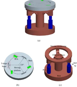
In order to implement more DOFs in a single plane, the in-plane 3-DOF (XYθz) precision positioning stage has been designed, and the translation along X- and Y- axes and rotation about Z- axis movements can be realized. As shown in Fig.1 (b), the stage is mainly composed of three piezoelectric actuators (PEAs), three T-shape flexible hinges, the moving platform and a base. Three flexible mechanisms based on flexible hinges are arranged in the same circle with the grooves, with the separated angle of 120° between them and 60° with grooves, respectively. Each T-type flexible mechanism is composed of three leaf-spring hinges, which is connected to the base and the moving platform at each end of the flexure hinge.

(a)

(b) (c)

Fig. 1.(a) Schematic diagram of the 6-DOF positioning system, (b) the in-plane parallel stage and (c) the out-of-plane parallel stage

Fig. 1(c). It is mainly composed of three piezoelectric actuators (PEAs), three elliptical flexible hinges, a moving circular ring and a base with central column. Three parallel PEAs are secured with axial symmetry around the circumference of a cylindrical base and press against the elliptical flexible hinges through ball tips. The end of each PEA is connected to the base by the bolt preload to ensure that the PEAs are fixed with the base and the hinges is not separated during normal operation. Because of the brittle characteristic of piezoelectric materials, the actuators are strong enough against compressive force, but weak against shear force. The actuators cannot supply lateral stiffness and are liable to be damaged from lateral forces. To solve this problem, drive ball tips mounted onto the actuators push against the hinges under Hertzian contact conditions.

the present in-plane precision positioning stages have not been satisfactory carrying capacity, and the carrying capacity of the out-of-plane precision positioning stage is better than the in-plane in generally. Therefore, this design idea in references [26], [28] and [29] is not suitable from viewpoints of both positioning accuracy and fast positioning response speed. For the above reasons, we proposed a novel 6-DOF precision positioning stages, which is assembled by two type 3-DOF precision positioning stages. The in-plane 3-DOF stage is mounted on the out-of-plane 3-DOF stage. Such kind of design will improve the stability of the system and ensure the good dynamic characteristics, higher stability, faster response speed and high-accuracy positioning.

2.2 Performance assessment

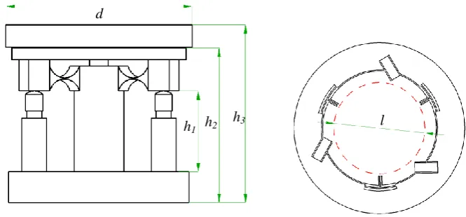
Based on the conceptual design, as shown in Fig. 2, the 6-DOF system is designed with the main parameters: d = 150 mm, h1 = 65 mm, h2 = 125 mm, h3 = 143 mm, and l = 80 mm (The diameter of the work area). The thickness of the T-type and elliptical flexible hinges t = 1 mm.

Fig. 2.Geometric model of the 6-DOF system

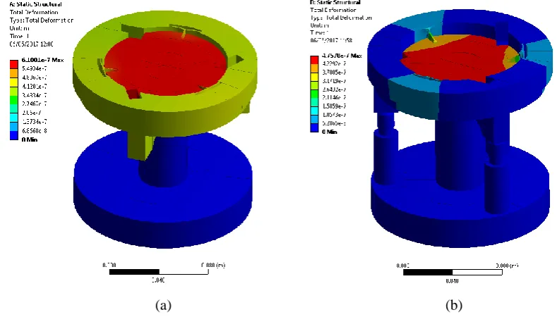
In order to assess the performance of the 6-DOF system and verify the accuracy of the established models, Finite element analysis (FEA) simulations are carried out with ANSYS software package. The material for the in-plane stage is chosen as Aluminum 7075-T6 with a density of 2770 kg/m3, a Young's modulus of 71 GPa, a yield strength of 503 MPa and a Poisson's ratio of 0.33. And the material for the out-of-plane stage is chosen as Structural Steel with a density of 7800 kg/m3, a Young's modulus of 200 GPa, a yield strength of 430 MPa and a Poisson's ratio of 0.3. In order to improve the computational accuracy, the mapping mesh method is adopted. The mesh is strictly controlled in the areas of flexure hinges, where the large deformation is generally occurred.

d

h1 h2

To assess loading performance of the stage, the FEA simulation is carried out by applying an external load on the moving platform with a 12N force, the results are illustrated in Fig. 3, which shows a maximum deformation of the system without PEAs is 0.618 μm, and a maximum deformation of the system with PEAs is reduced to 0.475 μm. Additionally, the loading capacity is 19.42 and 25.26 N/μm in the Z direction also can be obtained, respectively.

(a) (b)

Fig. 3.The deformation of the 6-DOF positioning system under external load: (a) without PEAs and (b)

with PEAs

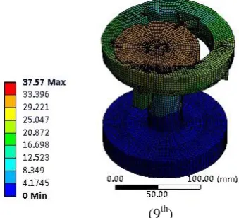
The dynamic characteristics of the 6-DOF system are investigated through the modal analysis and the results are shown in Fig. 4. The first, second and third modes shown that the moving platform rotates about the X-, Y- and Z- axis, respectively. The moving platform moves along the Z-axis in the fourth mode shape. The outer ring of the in-plane 3-DOF stage rotates about the Z-axis in the fifth mode. In the sixth and seventh modes the moving platform moves along the X- and Y-axis, it clear shown that the coupling motion in the 6-DOF system. In the eighth and ninth modes the moving platform moves along the X- and Y-axis, respectively. The corresponding frequencies of the modes are shown in Table I.

Table I. The corresponding frequencies of the mode shapes

Modal 1st 2nd 3rd 4th 5th

Frequency(Hz) 323.31 323.33 526.4 677.75 746.57

Modal 6th 7th 8th 9th

(1st) ₍₂nd

)

(3rd) (4th)

(5th) ₍₆th

)

Fig. 4.The first nine modes of the 6-DOF system without PEAs

3. Modeling

3.1 Kinematic model

In order to describe the kinematic model of the 6-DOF positioning system, the transformation matrix T is presented. The 6-DOF positioning system can achieve only one- or multi-direction positioning by six PEAs with different output displacements [41]. Referring to equation (1), the transformation matrix T between the input displacements matrix Г and output displacements matrix O can be expressed as:

O T

Γ   (1)

where, O=[x y α θx θy z]T, Г=[δ1 δ2 δ3 δ4 δ5 δ6]T. δ1, δ2, and δ3 are the elongation of the PEAs in the in-plane stage, and δ4, δ5, and δ6 are the elongation of the PEAs in the out-of-plane stage, respectively; x, y, z and α, θx, θy are the displacement in the X-, Y-, Z-axes and the rotation angle about the Z-, X-, Y-axes of the moving platform, respectively.

According to the geometrical relation, as shown in Fig. 5, a reference coordinate O-XYZ

is established. A moving coordinate Od-XdYdZd is located at the centre of the moving circular ring on the out-plane 3-DOF stage, which coincides with the fixed reference coordinate O-XYZ. The other coordinate frame Os-XsYsZs is located at the centre of the moving platform of the 3-DOF in-plane system. Through coordinate transformation, the transfer matrix Ts of the moving coordinate Os-XsYsZs relative to the reference coordinate O-XYZ can be obtained as follows:

         ) , ( ) , ( ) , ( ) , ( ) , ( ) , ( ) , (    z R T z Tran P y Tran P x Tran P z Tran y R x R z y x sd z y x d sd d s T T T T T (2)

where: the transfer matrix Td of the moving coordinate Od-XdYdZd relative to the reference coordinate O-XYZ has been rotated by θx, θy around the X- and Y-axis, and translated by Pz along the Z-axis, respectively. And the transformation matrix Tsd of the moving coordinate

Os-XsYsZs relative to the coordinate Od-XdYdZd has been translated by Px, Px and Tz along the

X-, Y- and Z-axis, respectively, and rotated by α around the Z-axis. Therefore, the transfer matrix Ts can be obtained,

                            1 0 0 0 z y x z x y y x x y x x y x x y x y x z x y y x x y x x y x x y x y z y x y y x y x s P c c T s P s c P c c c s s s c s s c s c c s T c P s s P c s c c s s s s c c s s s T c P s c s c c                                          T

where s=sin, c=cos. Then, the displacement of the origin point Os of Os-XsYsZs relative to the reference coordinate O-XYZ can be written as follows:

                                z y x z x y y x x y x z x y y x x y z y x P c c T s P s c P c s T c P s s P s T c P z y x             (3)

Owing to small values of θx and θy, it can be deduced that sinθx(θy)≈θx(θy), cosθx(θy)≈1. Meanwhile, infinitesimal of higher orders are neglected. Therefore, the equation (3) can be written as:           z P T y P T x P z z x y z y x   (4)

According to the kinematic analysis model of the in-plane 3-DOF stage [42] and out-of-plane 3-DOF stage [43]. The (4) can be written as:

(a) Front view (b) Top view

Fig. 5. Geometric model of the 6-DOF system without PEAs

Therefore, the relation can be obtained:

                                                                                                             z y x T T R R R R R r r r y x z z          1 0 0 0 0 0 0 1 0 0 0 0 0 0 1 0 0 0 0 0 0 1 0 0 0 0 0 1 0 0 0 0 0 1 3 1 3 1 3 1 0 0 0 3 2 3 1 3 1 0 0 0 0 3 3 3 3 0 0 0 0 0 0 3 1 3 1 3 1 0 0 0 3 1 3 1 3 2 0 0 0 3 1 3 1 0 6 5 4 3 2 1 (6)

And then, the transformation matrices T be expressed as follows:

                                     1 0 0 0 0 1 2 2 3 0 0 0 1 2 2 3 0 0 0 0 2 3 2 2 1 2 3 0 2 3 2 2 1 2 3 0 0 1 0 R R R R R T T r T T r T r z z z z z T (7)

And TTT can be given as follow: Zs

Os Xs

X Tz (O_d) O

(Xd)

(Zd) Z

Os

Ys

Xs

                               3 0 0 0 0 0 0 2 ) ( 3 0 0 0 2 3 0 0 2 ) ( 3 0 2 3 0 0 0 0 3 0 0 0 0 2 3 0 2 3 0 0 2 3 0 0 0 2 3 2 2 2 2 2 T R T T R T T r T T z z z z z z T T (8)

3.2 Dynamic model

In order to establish dynamic model, the 6-DOF system can be modeled as a multi-spring-mass system. kx and kzare considered to be the equivalent linear stiffness in the X and Z-axes of the 6-DOF system, respectively. cx and cy denote the equivalent damping coefficient in the X and Z-axes of the 6-DOF system, respectively. According to the matrix of

TTT, the stiffness matrix K of the 6-DOF system can be written as:

                               z z z x z z z x z x z z x z z x k k R T k T k R T k T k r k T k k T k 3 0 0 0 0 0 0 2 ) ( 3 0 0 0 2 3 0 0 2 ) ( 3 0 2 3 0 0 0 0 3 0 0 0 0 2 3 0 2 3 0 0 2 3 0 0 0 2 3 2 2 2 2 2 K

Similarly, the damping matrix C of the 6-DOF system also can be obtained.

Based on the second Newton’s second law of motion, the differential equations for dynamic motion of the system are given as follows:

QF q K q C q

M  _T  _T 

2 3 2 3     where: ) (m m I I I m

diag z x y



M 





z y

x  _x _y

 q  ) 2 ) ( ) ( 2

( 2 2 2 2 2

z z z x z z z x z x z z x z z x

T diag k Tk k Tk r k Tk  T R k Tk  T R k k

can be obtained by the stiffness matrix K of the system, and the motions can be considered already decoupled.  ) 2 ) ( ) ( 2

( x z z x z z 2 x z x z2 2 z z x z2 2 z z

T diag c Tc c Tc r c Tc  T R c Tc  T R c c

C _





6 5 4 3 2

1 p p p p p

p f f f f f

f  F                                       1 1 1 0 0 0 2 2 2 3 2 3 0 0 2 3 2 3 2 2 0 0 0 0 0 0 2 1 2 1 1 0 0 0 2 3 2 3 0 R R R T T R R T T T r r r z z z z z Q 

where: m is the equivalent mass, Ix, Iyand Izdenote the equivalent moment of inertia about the X, Y and Z-axes, respectively. fpi (i=1,2,3,4,5,6) represents the equivalent driving force of the PEA. And r is the radius of the moving platform, R is the radius of the moving circular ring.

The equivalent linear stiffness kx and kz can be expressed as:

              c pzt c pzt jz z c pzt c pzt jx x k k k k k k k k k k k k 

where: kjxand kjzare the equivalent linear stiffness in the X and Z-axes of the flexible hinges, respectively. kpzt is the equivalent stiffness of PEA, kc is the equivalent Hertzian contact stiffness.

To ensure that the PEAs and the moving platform are not separated during normal operation, the PEAs are installed in slots and connected to the base by the bolt preload. Therefore, the driving force of PEA can be obtained:





 

 k dV i

k k

k k

f _{amp e pzt}

c pzt

c pzt

pi 

where: de is a piezoelectric constant, Vpztis the applied voltage, and kamp is an amplification coefficient.

PF Gq q D

q   

where: ) 2 2 2 2 2 2

( _{x nx y ny n x n x y n y z nz}

diag         



D 

)

( 2 2 2 2 2 2

nz y n x n n ny nx

diag      

    G  Q M

P 1 _

m k k R T k T I k R T k T I r I k k T k m k T k m z nz z z x z y n z z x z x n z x n z z x ny z z x nx y x 3 ), ) ( ( 2 3 ), ) ( ( 2 3 3 ), ( 2 3 ), ( 2 3 2 2 2 2 2 2 2 2 2 2 2                       m c c R T c T I c R T c T I r I c c T c m ， c T c m z nz nz z z x z y n z z x z x n z x n z z x ny y z z x nx x y y x x 3 2 ), ) ( ( 2 3 2 ), ) ( ( 2 3 2 3 2 ), ( 2 3 2 ) ( 2 3 2 2 2 2 2 2 2                                

4. Design of a Control Scheme

In order to overcome the positioning error caused by the hysteresis and nonlinear behaviour of PEAs [44] this section presents the design of DMPC (Discrete-time Model Predictive Controller) control scheme undertaken in this work. The proposed DMPC control technique is designed to reduce the tracking error problem and improve the positioning accuracy of the 6-DOF system. The schematic diagram of the closed-loop control system is shown in Fig. 6. The inverse kinematic matrix is the matrix T in the section 3. The DMPC scheme is employed to design a tracking controller in which the output tracks a reference desired input. Its basic structure of DMPC is shown in Fig. 7. The DMPC utilizes the system model to predict the system's future outputs based on the current values of the system output and the future values of its inputs. Then, rolling optimization is implemented, a predefined cost function and constraints are took into account, which ensure the predicted output is close enough to the reference trajectory, and simultaneously eliminates the possibility of variables exceeding their allowable range [45].

       ) ( ) ( ) ( ) ( ) 1 ( k x C k y k u B k x A k x m m m m m m (13)

where Am, Bm and Cm are the discrete state-space system model, which can be extracted from the system differential equations by (12), u is the input variable, y is the predicted output, x is the state variable vector with dimension n. From the original dynamic equation (9), the state-space model can be written as:

 

T _M K _{M Q}

C M

 

(14)

In order to restrain the interference and track a reference signal in the DMPC algorithm, it needs to change the model to suit the design purpose in which an integrator is embedded, the system model can be augmented in the following way [37]:

                                ) ( ) ( ) ( ) ( ) ( ) ( ) 1 ( ) 1 ( k y k x C k y k u B k y k x A k y k x m m m (15)

where A, B and C are the augmented system matrices.

       I A C A A m m m 0        m m m B C B

B C





) 1 ( ) ( ) ( ), ( ) 1 ( ) 1 ( ), 1 ( ) ( ) (              k x k x k x k x k x k x k u k u k u m m m m m m

Form (14), matrix A and B can be obtained:

                                                    0 0 1 1 0 0 2 3 2 3 0 1 0 0 1 1 1 e amp c pzt c pzt m m m T T m m m d k k k k k B C B B I A C A A Q M K M C M

) 1 ( ) ( ) ( ) ( ) 1 ( ) ( ) ( ) 2 ( ) ( ) ( ) 1 ( 1 2                       c N N N N p N k u B A k u B A k x A k N k x k u B k u AB k x A k k x k u B k Ax k k x c p p p _ 

where Np is the prediction horizon and Nc is the control horizon. According to the predicted state variables, the predicted output variables are,

) 1 ( ) ( ) ( ) ( ) 1 ( ) ( ) ( ) 2 ( ) ( ) ( ) 1 ( 1 2                       c N N N N p N k u B CA k u B CA k x CA k N k y k u CB k u CAB k x CA k k y k u CB k CAx k k y c p p p _ 

The output sequence on Np, prediction horizon can be written as follows:

ΦΔU F

Y x(k) (16)

in which,

Fig. 7.Structure of the DMPC













To obtain a best control input meeting various conditions, rolling optimization is implemented to ensure that the predicted output is close enough to the reference trajectory, and simultaneously to reduce the vibration of the 6-DOF system caused by possible severe control changes. The cost function J reflecting the control objective is defined as follows:





 p Nc

m T N m s T

s Y R Y U C U

R J 1 1 ˆ ) ( )

( (17) where Rs=INp×1rk is a given reference signal, Ĉ is a diagonal matrix in the form that

Ĉ=rwINc×Nc, rw (rw≥0) is used as a tuning parameter for the desired closed-loop performance. The first term is linked to the objective of minimizing the errors between the predicted output and the reference signal while the second term reflects the consideration given to the size of

∆U when the objective function J is made to be as small as possible [46]. Subject to the linear inequality constraints on the system inputs

c c N i u i k u u N i u i k u u , , 1 , ) 1 ( , , 1 , ) 1 ( max min max min                (18)

To ensure J to reach its minimum, its partial derivative needs to satisfy the following constraint: 0 ) ˆ ( 2 )) ( (

2      

     U C k Fx R U J T s T (19)

Thus the solution of the optimal input ∆U:

)) ( (

) ˆ

( C 1 R Fx k

U T T _s 

 

5. Experiment and Results

The developed prototype of 6-DOF positioning stage is shown in Fig. 8. The top and bottom surfaces of the two 3-DOF stage are fabricated on a milling machine, respectively. Subsequently, artificial aging is utilized to release the residual stress. Computer numerical control (CNC) assisted wire electrical discharge the machining (WEDM) technique is utilized to manufacture all the flexure structures. During the WEDM fabrication process, low-speed feeding is selected to guarantee the machining accuracy, and a fabrication tolerance of 2 μm is achieved. Both of the stages are bolted together. Three AE0505D18F (THORLABS) and three PI P-844.10 (Physik Instrumente) PEAs were used to actuate the in-plane stage and out-of-plane stage, respectively.

As shown in Fig. 9, three AE0505D18F (THORLABS) and three PI P-844.10 (Physik Instrumente) PEAs were used with the maximum displacement of 15µm under the input voltage of 100V, which were used to actuate the in-plane stage and out-of-plane stage, respectively. The dSPACE DS1103 controller (dSPACE Ltd) was used to generate the controlling signal, the PI E-505.00 amplifier (Physik Instrumente) and 3-Axls Piezo Controller THORLABS MDT693B were used to amplify the signal then drive the PEAs. Three KEYENCE laser displacement sensors LK-H050 and three capacity position sensors D-050.00 (Physik Instrumente) were used to measure the motion of the in-plane and out-of-plane stage, respectively. The amplifier E-509.C3A (Physik Instrumente) for capacity position sensors was installed in a chassis. In order to reduce the external disturbance effects on the testing system, the 6-DOF system is mounted on a Newport RS-4000 optical table.

Fig. 8.Manufactured prototype of 6-DOF positioning stage

Fig. 9.Experimental setup of the system

5.1Step Responses and Motion Range

The step responses of the system are investigated, and the step responses in the X-, Y- and Z- axes directions are shown in Fig. 10. The result shows that the 2% settling time of the step responses are 34, 41 and 62 ms, respectively. The effective motion range is also validated, the stroke of the movement were 8.2μm in the X-axis, 10.5μm in the Y-axis, 13.2μm in the Z-axis, 225μrad in the θz-axis, 107μrad in the θx-axis and 100μrad in the θ y-axis, respectively.

(a) (b)

(c)

5.2Resolution

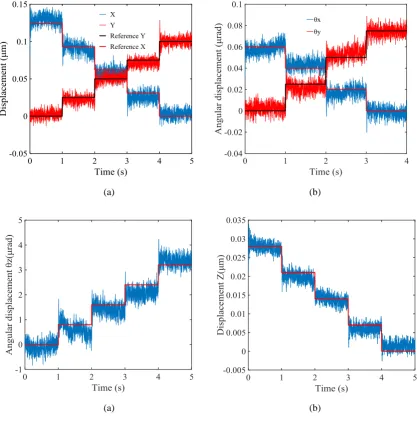
Precision motion is tested. As can be seen in Fig. 11, the minimum resolutions are clearly resolved from the multi-step response experiment, which as regards six stability measures are 31 nm in the X-axis, 25nm in the Y-axis, 7nm in the Z-axis, 0.8μrad in the θz-axis, 20nrad in the θx-axis and 25nrad in the θy-axis, respectively. In this test, the movement of the platform is measured in 6-DOF by two type capacitance sensors, the resolution of three KEYENCE laser displacement sensors are lower than three capacity position sensors D-050.00. If the resolution of the displacement sensor can be improved and the external disturbance signal will be further reduced, a higher resolution of the developed positioning system can be achieved.

(a) (b)

(a) (b)

5.3Controller Verification

In the control experiments, the sampling time interval is assigned as t=0.0001s. In order to verify the effectiveness of the DMCP control method, some comparative testes are performed. For a reference sinusoidal trajectory (Y-axis), as shown in Fig. 12(a), the different results of PID and DMCP control are both shown in Fig. 12(a), and the two tracking errors also are clearly depicted. The PID feedback control gives a max-error of 2.16% with respect to the motion range. By contrast, the control using DMPC produces a max-error of 1.20%. It is seen that DMPC achieves better results than PID. Besides, for a reference bi-axial circular trajectory, as shown in Figs. 12(b), (c) and (d), the results indicate that the PID control scheme leads to a errors of 3.96% in the X-axis and 2.44% in the Y-axis, and the max-errors of 1.86% in the X-axis and 1.62% in the Y-axis can be achieved by employing DMPC control scheme, respectively. Compared to the PID control scheme, DMPC control reduces the tracking errors in the X-, Y-axes by 53% and 34.1%, respectively.

For a clear comparison, the effectiveness of DMPC control is evident from the control results, which suppresses the maximum tracking errors by above 34%, as compared with the traditional PID control scheme. It also confirms the effectiveness of DMPC control approach on improving the tracking performance compared to traditional PID. This means that it can be applied to reduce the tracking error and improve the positioning accuracy of the 6-DOF system.

(b)

(c)

(d)

Fig. 12. The result of motion tracking with two diffrent contorl methods. (a) Sinusoidal trajectory. (b) Circular trajectory. (c) Tracking error (DMPC). (D) Tracking error (PID).

5.4Tracking Performance

To test the tracking ability of the 6-DOF system under the control block diagram, six sinusoidal trajectory motion tests are conducted to evaluate the tracking performance of the 6-DOF system. Fig. 13 shows the experimental results on the six sinusoidal trajectories. As shown in Fig. 13, the maximum tracking errors is ±0.06 μm, which with respect to the output displacement is as small as 1.2%. For three rotational DOF trajectories, The maximum tracking errors (±3.71 μrad, +2.56 μrad and -3.12 μrad) are observed in the motion, which with respect to the angular displacement is as large as 2.06%, 3.2% and 3.9%, respectively.

trajectories centered at point (2.5 μm, 2.5 μm) with a radius of 2.5 μm; b) Two complex trajectories are chosen as the reference trajectories defined by Eq. (21) and pentagon, respectively. c) A three-translational DOF trajectory is chosen as the reference trajectory defined by Eq. (22).

(a) (b)

(e) (f)

Fig. 13. The result of 1 Hz sinusoidal motion tracking

  

 



 

 



) 8 sin( ) sin( 2 3 ) (

) 5 . 0 8 sin( ) 5 . 0 sin( 2 3 ) (

t t

t y

t t

t x

 

 

 

 

    

  



 



t t

z

t t

y

t t

x

8 . 0 ) (

) 5 . 1 2 sin( 3 3 ) (

) 2 2 sin( 3 3 ) (

 

 



From the experimental result of bi-axial circular trajectories tracking, as shown in Fig. 14(a), the maximum tracking error (-0.093 μm in the X axis and -0.081 μm in the Y axis) with respect to the output displacement is as large as 1.86% in the X axis and 1.62% in the Y axis, respectively. As shown in Fig. 14(b), the maximum tracking error (-0.078 μm in the Y axis and -0.063 μm in the Z axis) with respect to the output displacement is as large as 1.56% in the Y axis and 1.26% in the Z axis, respectively.

However, for the complex trajectories, as shown in Fig. 15(a), compared with the circular trajectories, it is found that the tracking performance is unsatisfactory and obviously increased in tracking error. The maximum tracking error (0.115 μm in the X axis and 0.103 μm in the Y axis) with respect to the output displacement is as large as 1.92% in the X axis and 1.72% in the Y axis, respectively. As shown in Fig. 15(b), the maximum tracking error (-0.112 μm in the X axis and -0.099 μm in the Z axis) with respect to the output displacement is as large as 1.87% in the X axis and 1.65% in the Z axis, respectively.

The experimental result is shown in Fig. 16. It provided the discrepancies between the desired and actual trajectory. The tracking errors in the X-, Y- and Z- axis are also recorded, respectively. For the three-translational DOF trajectory (the helical trajectory), the maximum tracking error (-0.136 μm in the X axis, -0.117 μm in the Y axis and -0.093 μm in the Z axis) with respect to the output displacement is as large as 2.26% in the X axis, 1.95% in the Y axis and 1.55% in the Z axis, respectively.

(a) (b)

Fig. 14. The result of circular trajectory tracking

(a) (b)

Fig. 16. The result of the helical trajectory motion tracking

6. Conclusion

control method. The tracking experiment is performed to verify the tracking performances of the 6-DOF stage. And the collected experimental results show that the proposed 6-DOF stage has a good tracking performance.

Acknowledgement

This work was supported by the National Natural Science Foundation of China (No. 51505330, 51675371, 51420105007), EU H2020 MSCA RISE 2016 (No.734174) and China Scholarship Council (Grant No. 201606250048).

References

[1] B. Choi, S. Sreenivasan, S. Johnson, et al., “Design of orientation stages for step and flash imprint

lithography,” Precision Engineering, vol. 25, no. 3, pp. 192-199, Jul. 2001.

[2] M. Zareinejad, S. M. Rezaei, A. Abdullah, et al., “Development of a piezo-actuated micro-teleoperation

system for cell manipulation,” The international Journal of Medical Robotics and computer Assisted

Surgery, vol. 5, no. 1, pp. 66-76, Mar. 2009.

[3] O. Payton, L. Picco, A. Champneys, et al., “Experimental observation of contact mode cantilever dynamics

with nanosecond resolution,” Review of Scientific Instruments, vol. 82, no. 4, 043704, pp. 1-5, Apr. 2011.

[4] W. Yang, S. Lee and B. You, “A piezoelectric actuator with a motion-decoupling amplifier for optical disk

drives,” Smart Materials and Structures, vol. 19, no. 6, 065027 pp. 1-10, Jun. 2010.

[5] J. Moon, H. Pahk and B. Lee, “Design, modeling, and testing of a novel 6-DOF micropositioning stage with

low profile and low parasitic motion,” International Journal of Advanced Manufacturing Technology, vol.

55, no. 1-4, pp. 163-176, Jul. 2011.

[6] T. Secord and H. H. Asada, “A variable stiffness PZT actuator having tunable resonant frequencies,” IEEE

Transactions on Robotics, vol. 26, no. 6, pp. 993-1005, Dec. 2010.

[7] D. Wang, Q. Yang and H. Dong, “A monolithic compliant piezoelectric- driven microgripper: design,

modeling, and testing,” IEEE/ASME Transactions on Mechatronics, vol. 18, no. 1, pp. 138-147, Feb. 2013.

[8] M. Zubir, B. Shirinzadeh and Y. Tian, “A new design of piezoelectric driven compliant-based microgripper

for micromanipulation,” Mechanism and Machine Theory, vol. 44, no. 12, pp. 2248-2264, Dec. 2009.

[9] M. Raghavendra, A. Kumar and B. Jagdish, “Design and analysis of flexure-hinge parameter in

microgripper,” International Journal of Advanced Manufacturing Technology, vol. 49, no. 9-12, pp.

1185-1193, Aug. 2010.

[10]Y. Tian, B. Shirinzadeh, D. Zhang, “A flexure-based mechanism and control methodology for

[11]Y. Tian, B. Shirinzadeh, D. Zhang, “Design and dynamics of a 3-DOF flexure-based parallel mechanism

for micro/nano manipulation,” Microelectronic Engineering, vol. 87, no. 2, pp. 230-241, Feb. 2010.

[12]Y. Qin, B. Shirinzadeh, Y. Tian, D. Zhang and U. Bhagat, “Design and Computational Optimization of

aDecoupled 2-DOF Monolithic Mechanism,” IEEE/ASME Transactions on Mechatronics, vol. 19, no. 3, pp.

872-881, Jun. 2014.

[13]Y. Qin, B. Shirinzadeh, Y. Tian, D. Zhang, “Design issues in a decoupled XY stage: Static and dynamics

modeling, hysteresis compensation, and tracking control,” Sensors and Actuators A: Physical, vol. 194, no.

1, pp. 95-105, May. 2013.

[14]D. Zhang, D.G. Chetwynd, X. Liu, Y. Tian, “Investigation of a 3-DOF micro-positioning table for surface

grinding,” International Journal of Mechanical Sciences, vol. 48, no. 12, pp. 1401-1408, Dec. 2006.

[15]H. Kim, J. Kim, D. Ahn, D. Gweon, “Development of a Nanoprecision 3-DOF Vertical Positioning System

With a Flexure Hinge,” IEEE Transactions on Nanotechnology, vol. 12, no. 2, pp. 234-245, Mar. 2013.

[16]H. Lee, H. Kim, H. g Kim, D. Gweon, “Optimal design and experiment of a three-axis out-of-plane nano

positioning stage using a new compact bridge-type displacement amplifier,” Review of Scientific

Instruments, vol. 84, no. 11,115103, pp. 1-10, Nov. 2013.

[17]D. Kim, D. Kang, J. Shim, I. Song, D. Gweon, “Optimal design of a flexure hinge-based XYZ atomic force

microscopy scanner for minimizing Abbe errors,” Review of Scientific Instruments, vol. 76, no. 7,073706,

pp. 1-7, Jul. 2005.

[18]M. Lu, S. Gao, Q. Jin, J. Cui, H. Du, H. Gao, “An atomic force microscope head designed for

nanometrology,” Measurement Science and Technology, vol. 18, no. 6, pp.1735-1739, 2007.

[19]M. Taniguchi, M. Ikrda, A. Inagaki, “Ulta precision wafer positioning by six-axis micro-motion

mechanism,” Int. J. Jpn. Soc. Precis. Eng. vol. 26, no.1, pp. 35-40, 1992.

[20]T. Tanikawa, T. Arai, P. Ojala, “Two-finger micro hand,” In: Proc. of the IEEE Int. Conf. on Robot. and

Auto., Leuven, Belgium, pp. 1674-1679, 1995.

[21]N. Fazenda, E. Lubrano, S. Rossopoulos, R. Clavel, “Calibration of the 6 DOF high-precision flexure

parallel robot “Sigma 6”,” In: 5th Chemnitzer Parallelkinematik Seminar, pp. 379-398, Chemnitz, 2006.

[22]Thomas H. Vose, Matthew H. Turpin, Philip M. Dames, Paul Umbanhowar, Kevin M. Lynch, “Modeling,

design, and control of 6-DoF flexure-based parallel mechanisms for vibratory manipulation,” Mechanism

and Machine Theory, vol. 64, pp. 111-130, 2013.

[23] Q. Liang, D. Zhang, Z. Chi, Q. Song, Y. Ge, Y. Ge, “Six-DOF micro-manipulator based on compliant

parallel mechanism with integrated force sensor,” Robotics and Computer-Integrated Manufacturing, vol.

27, no. 1, pp. 124-134, Feb. 2011.

[24]L. Tsai, S. Joshi, “Kinematic analysis of 3-dof position mechanisms for use in hybrid kinematic machines,”

ASMEJ. Mech. Des. vol. 124, no. 2, pp. 245-253, 2002.

[25]G. Yang, W. Chen, H. Hui, “Design and kinematic analysis of a modular hybrid parallel-serial manipulator,”

In: Proc. Of the ICARCV02, vol. 1, pp. 45-50, 2002.

[26]P. Gao, S. Swei, “A six-degree-of-freedom micro-manipulator based on piezoelectric translators,”

Nanotechnology, vol. 10, no. 4, pp. 447-452, 1999.

[27]R. Seugling, T. LeBrun, S. Smith, L. Howard, “A six-degree-of-freedom precision motion stage,” Review

[28]R. Fung, W. Lin, “System identification of a novel 6-DOF precision positioning table,” Sensors and

Actuators A: Physical, vol. 150, no. 2, pp. 286-295, Mar. 2009.

[29]D.H. Chao, G.H. Zong, R. Liu, “Design of a 6-DOF com-pliant manipulator based on serial-parallel

architecture,” In: IEEE/ASME Int. Conf. Adv. Intell. Mechatron., Monterey, CA, USA, pp. 765-770, 2005.

[30]A. Boukari, J. Carmona, G. Moraru, F. Malburet, A. Chaaba, M. Douimi, “Piezoactuators modeling for

smart applications,” Mechatronics, vol. 21, no. 1, pp. 339-349, Feb. 2011.

[31]L. Juhasz, J. Maas, B. Borovac, “Parameter identification and hysteresis compensation of embedded

piezoelectric stack actuators,” Mechatronics, vol. 21, no. 1, pp. 329-338, Feb. 2011.

[32]C. Lin, P. Lin, “Tracking control of a biaxial piezo-actuated positioning stage using generalized Duhem

model,” Computers and Mathematics with Applications, vol. 64, no. 5, pp. 766-787, Sep. 2012.

[33]M. Rakotondrabe, “Bouc-Wen modeling and inverse multiplicative structure to compensate hysteresis

nonlinearity in piezoelectric actuators,” IEEE Transactions on Automation and Engineering, vol. 8, no. 2,

pp. 428-431, Apr. 2011.

[34]X. Zhang and Y. Lin, “Adaptive tracking control for a class of pure-feedback non-linear systems including

actuator hysteresis and dynamic uncertainties,” IET Control Theory and Applications, vol. 5, no. 16, pp.

1868-1880, Nov. 2011.

[35]M. Rakotondrabe, C. Clevy, and P. Lutz, “Robust feedforward-feedback control of a nonlinear and

oscillating 2-DOF piezocantilever,” IEEE Transactions on Automation Science and Engineering, vol. 8, no.

3, pp. 506-519, Jul. 2011.

[36]T. Tuma, A. Pantazi, J. Lygeros, and A. Sebastian, “Nanopositioning with impulsive state multiplication: A

hybrid control approach,” IEEE Transactions on Control Systems and Technology, vol. 21, no. 4, pp.

1352-1364, Jul. 2013.

[37]P. Ko, Y. Wang and S. Tien, “Inverse-feedforward and robust-feedback control for high-speed operation on

piezo-stages,” International Journal of Control, vol. 86, no. 2, pp. 197-209, Sep. 2012.

[38]M. S. Rana, H. R. Pota, and I. R. Petersen, “Model predictive control of atomic force microscope for fast

image scanning,” in 51st Conference on Decision and Control (CDC), Hawaii, USA, Dec. 2012, pp.

2477-2482.

[39]M. S. Rana, H. R. Pota, and I. R. Petersen, “High-speed AFM image scanning using observer-based

MPC-notch control,” IEEE Transactions on Nanotechnology, vol. 12, no. 2, pp. 246-254, Mar. 2013.

[40]Q. Xu and Y. Li, “Model predictive discrete-time sliding mode control of a nanopositioning piezostage

without modeling hysteresis,” IEEE Transactions on Control Systems and Technology, vol. 20, no. 4, pp.

983-994, Jul. 2012.

[41]K. Cai, Y. Tian, F. Wang, et al., “Design and control of a 6-degree-of-freedom precision positioning

system,” Robotics and Computer-Integrated Manufacturing, vol. 44, pp. 77-96, 2017.

[42]K. Cai, Y. Tian, F. Wang, D. Zhang, B. Shirinzadeh, “Development of a piezo-driven 3-DOF stage with

T-shape flexible hinge mechanism,” Robotics and Computer-Integrated Manufacturing, vol. 37, no. 1, pp.

125-138, Feb. 2016.

[43]D. Zhang, D.G. Chetwynd, X. Liu, Y. Tian, “Investigation of a 3-DOF micro-positioning table for surface

[44]M. Rakotondrabe, “Bouc-Wen modeling and inverse multiplicative structure to compensate hysteresis

nonlinearity in piezoelectric actuators,” IEEE Transactions on Automation and Engineering, vol. 8, no. 2,

pp. 428-431, Apr. 2011.

[45]L. Wang, Model Predictive Control System Design and Implementation Using MATLAB. London, UK:

Springer, 2009

[46]D. A. Linkers and M. Mahfonf, Advances in Model-Based Predictive Control, Chapter Generalised

Predictive Control in Clinical Anaesthesia. Oxford, U.K.: Oxford Univ. Press, 1994.

[47]N. Qi, Y. Fang, X. Ren, and Y. Wu, “Varying-Gain Modeling and Advanced DMPC Control of an AFM

System,” IEEE Transactions on Nanotechnology, vol. 14, no. 1, pp. 82-92, Jan. 2015.

[48]M. S. Rana, H. R. Potaand I. R. Petersen, “Performance of Sinusoidal Scanning With MPC in AFM

Imaging,” IEEE/ASME Transactions on Mechatronics, vol. 20, no. 1, pp. 73-83, Feb. 2015.

[49]K. Low and H. Zhuang, “Robust model predictive control and observer for direct drive applications,” IEEE