Abstract
This thesis describes a research on the impact of multiple searching Bluetooth devices on the Bluetooth discovery protocol.
Bluetooth is a standard which describes energy efficient wireless communi-cation. Because of its characteristics, most mobile devices incorporate Blue-tooth as their means of wireless inter-device communication. In order for two devices to communicate using Bluetooth, they first need to set up a connec-tion. A device can start a scan (inquiry scan) to discover available devices in the area. On a low level a device can be discovered without that device physically notifying its user. This principle is exploited to trace people as they move.
This research focusses on the discovery time when using multiple inquirers (searching devices). This discovery time influences the performance of a local-ization system. A series of experiments is set up to test this performance. A subset of these experiments are then used to create a model for modeling the discovery time for multiple inquirers. This model is based on the empirical data for one inquirer.
Contents
Abstract i
Contents ii
List of Figures iii
List of Tables iv
1 Introduction 1
1.1 Localization . . . 2
1.2 Bluetooth . . . 3
1.3 Problem statement . . . 4
1.4 Research questions and contributions . . . 4
1.5 Outline . . . 6
2 Introduction to Bluetooth 9 2.1 Introduction . . . 9
2.2 Data communication . . . 10
2.3 Inquiry process . . . 11
3 Bluetooth inquiry performance 15 3.1 Inquiry process parameters . . . 15
3.2 Experiment design . . . 18
3.3 Effect of dutycycles . . . 24
3.4 Effect of multiple devices . . . 27
3.5 Related work . . . 29
3.6 Discussion . . . 32
3.7 Conclusion . . . 37
4 Modeling discoveries 39 4.1 Experiment design . . . 40
4.2 Model using observation windows . . . 41
4.3 Model using FHS interval time . . . 50
4.4 Related Work . . . 57
4.5 Conclusion . . . 59
5 Conclusions 61 5.1 Bluetooth behavior . . . 61
5.2 Modeling the inquiry process . . . 62
5.3 Future work . . . 62
Bibliography 65 A Miscellaneous 69 A.1 Effect of distance in the experiment . . . 69
A.2 Crowd scanning . . . 71
A.3 Tools . . . 72
B MySQL tables 79 C Functions of automated measuring tool 81
List of Figures
1.1 Trilateration to determine a location . . . 21.2 Fingerprint example . . . 3
2.1 Inquiry and paging procedure . . . 10
2.2 Inquiry process per timeslot of inquirer . . . 11
2.3 Scan windows per scan interval . . . 12
2.4 Inquiry scanner behavior after FHS reply . . . 12
3.1 Dutycycle for (a,b,c) inquiry scan . . . 16
3.2 Distance versus perceived signal strength . . . 17
3.3 Novay basement . . . 21
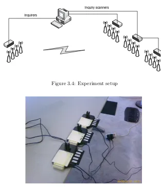
3.4 Experiment setup . . . 22
3.5 Novay basement with inquiry scanners . . . 22
3.6 MySQL table structure . . . 23
3.7 Congregation of dutycycles to ”observation window” . . . 25
3.8 Time to discovery of inq. scanners, for different dutycycles . . . . 26
3.9 Figure 3.8c expressed in percentages . . . 26
3.10 Figure 3.9 interpreted using a 6000ms observation window . . . 27
3.11 Time to discovery of inq. scanners, for different number of inquirers 27 3.12 Time to discovery of different amounts of inq. scanners . . . 28
3.13 Time to discovery of different amounts of inq. scanners, in percentages 28 3.14 Time to discovery at different distances, in percentages . . . 29
3.15 FHS packets per dutycycle . . . 33
3.16 Simulated probability density for inquiry scan from [22] . . . 33
3.17 Inquiry scanner behavior after FHS reply . . . 35
3.18 FHS Delay . . . 35
3.19 Delays between inquirers and application . . . 36
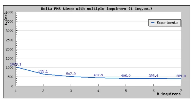
4.1 Inquirer dependent discovery times . . . 39
4.2 Experiment setup . . . 40
4.3 FHS Delays of new experiment . . . 41
4.4 Inquirer dependent discovery times, including modeled version (light-blue) . . . 44
4.5 Inquirer dependent discovery times, including 320ms model lower bound (lightblue) . . . 44
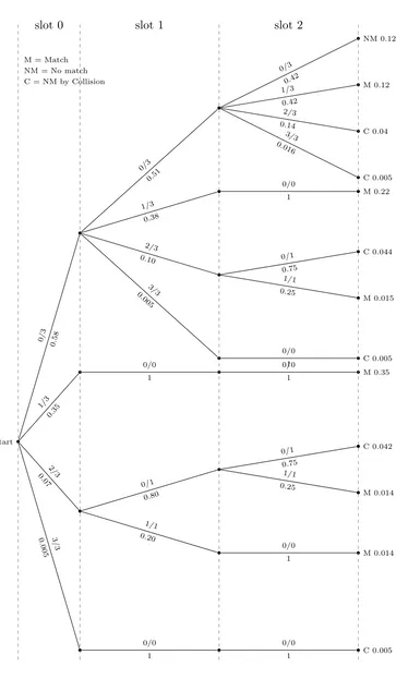
4.6 Collision probability tree . . . 46
4.7 Collision probability, 20 inquirers . . . 47
4.8 Collision probability, 200 inquirers . . . 47
4.9 Inquirer dependent discovery times, including collision probabilities 49 4.10 Average FHS interval times . . . 51
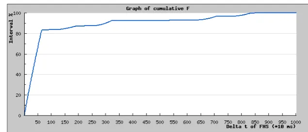
4.11 Cumulative probability density function of F . . . 53
4.12 Cumulative scaled pdf of D+ . . . . 53
4.13 Cumulative pdf of D− . . . 54
4.14 Cumulative pdf of D−, with average . . . . 54
4.15 Cumulative pdf of D+for multiple inquirers . . . 55
4.16 Cumulative pdf of D−for multiple inquirers . . . 56
4.17 Average FHS interval times including F+and F− . . . . 56
A.1 RSSI values relative to distance . . . 70
A.2 RSSI deviation over time [23] . . . 70
A.3 RSSI values relative to distance, positive logarithmic scale . . . 71
A.4 RSSI regression analysis (equation A.4), positive logarithmic scale 71 A.5 Web service, screenshot of index . . . 75
A.6 Web service, screenshot of experiment, discovered devices . . . 75
A.7 Web service, screenshot of experiment, fhs packets . . . 75
A.8 Web service, screenshot of experiment, fhs histogram . . . 76
A.9 Web service, screenshot of experiment, combined fhs histogram . . 76
A.10 Web service, screenshot of experiment, fhs histogram per inquirer . 77 A.11 Web service, screenshot of experiment, inquirer correlation . . . . 77
List of Tables
2.1 Bluetooth classes . . . 93.1 Parameters for dutycycle experiments . . . 20
3.2 Parameters for other experiments . . . 20
A.1 Bluetooth enabled people . . . 72
B.1 Structure of table crowdscanner . . . 79
List of Tables
B.2 Structure of table devices . . . 79
B.3 Structure of table dutycycles . . . 79
B.3 Structure of table dutycycles (continued) . . . 80
B.4 Structure of table experiments . . . 80
B.5 Structure of table manufacturers . . . 80
1
Introduction
Suppose there is a large, multi-story department store at which a lot of different items are sold. It might even include a restaurant. Having a system that could track customers as they move around the store would have several advantages;
• one can determine the route customers most often take
• one can determine which set of products are most popular by evaluating waiting-times
• one can have an informed push-offer-on-demand system, to give clients that appear to be in doubt (by detecting that they stand at an area for a long time) a coupon via Bluetooth, which is for example only valid for ten minutes.
• and consecutively the client behavior can be identified. For example: people that come to eat in the restaurant, which products are they most interested in?
These kinds of behavioral aspects of clients could be very important for a marketing-strategic business plan. It would be known exactly how to set up the departments in a store, which adverts to place in which sections, etc.
1. Introduction
Figure 1.1: Trilateration to determine a location
1.1
Localization
For a long time people have had a wish for having some form of localization. Maps show that people have always had the wish to know their own position. Navigation based on stars, already used by the Egyptians, was the primary means of localization for many centuries.
Digital localization is a topic which acquired general attention in 1983 when U.S. president Reagan declassified the Global Positioning System (GPS). From that day on, consumers where able to use global satellite localization with a precision of about 100 meters due to Selective Availability (SA [36]). This military restriction was finally lifted in the year 2000, making civilian GPS precision of 10-15 meters possible. On a global level, it is therefore now possible to calculate ones own position. Despite outdoor localization, indoor localization is still a challenge.
There are two categories in which localization systems can be divided [6]:
• Signal based. This technique uses analysis of the properties of the wireless signal itself to calculate the position of the device. These signal properties include lateration, angulation and proximity detection [32]. GPS is processing based localization; it uses lateration and angulation techniques to determine positions by processing different parameters of the radio signals (e.g. RSS, angle of arrival, time of arrival, ∆ time of arrival) [39].
Example:
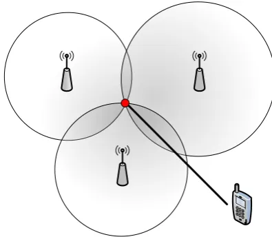
Trilateration can be used to determine the position of a mobile phone. By estimating the distances of the cell phone from three different base stations, the approximate intersection of these distances indicate the position of the cell phone (see figure 1.1). This distance is measured by determining the difference in the
1.2. Bluetooth
Figure 1.2: Fingerprint example
arrival-time of the signals of the mobile phone for each base station.
• Fingerprint based. Systems like this capture fingerprints of (some of the) known locations during an initial training phase. The network-characteristics of a device measured at each location are stored as a fin-gerprint. The measurement of a new device can be matched to these fingerprints. The best match determines the most likely location of the device. A fingerprint can for example consist of the IDs of the access points that are in range at a specific location.
Example:
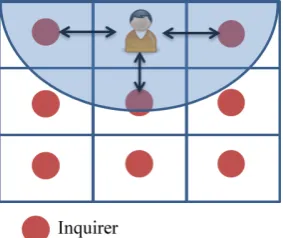
Figure 1.2 shows a building with different rooms. Each room has its own inquirer. In the room at the top, a device is located. Because the range of this device is limited, it can only detect several access points from that room (within the drawn range). In the database it is known which fingerprint belongs to that room, i.e. which access points can be seen by the devices that are in that particular room. The combination of access points in the drawn range can see the device. By looking up this com-bination of access points in the database, it can be established that the user must be in that room.
It is also possible for other ’processing based’ radio information to be used. By combining for example the access points with RSSI values can yield more accurate results if done properly.
1.2
Bluetooth
1. Introduction
Other types of technology have also been explored in other research, such as GSM [25] and 802.11 (Wireless LAN) [11]. The latter unfortunately means that the traced object or person should carry an 802.11 enabled device. The first one might be of interest, but Bluetooth provides other significant advantages. GSM based localization is less accurate than Bluetooth localization, and does not work well in indoor environments. With Bluetooth it is possible to push software-objects to a device, enabling intelligent advertisement and potentially customer interaction [18]. Furthermore, it means operating in a freely available frequency-band, with hardware that can easily and cheaply be obtained at any computer store. By making these design choices, hopefully the project will lead to a relatively cheap and easy maintainable localization system, being able to trace all people that have Bluetooth enabled on their mobile devices.
BlueWhere relies heavily on the discovery (inquiry) process of Bluetooth. Because Bluetooth uses several frequencies to communicate, two devices must first synchronize the frequency on which they can do so [26]. The inquiry pro-cess is the way in which two devices can discover eachothers presence. It is this process that can be used to scan for people with Bluetooth enabled devices. Whereas the people carry the devices that have to be found (inquiry scanners), the localization system provides the devices that search for those devices (in-quirers). When using more inquirers, inquiry scanners can be discovered faster up to a certain point. This principle is of great importance in this research. The next section discusses the problem statement.
1.3
Problem statement
An important issue in Bluetooth-based localization and tracing systems is the (adverse) impact of multiple Bluetooth devices on the performance of such systems. Several researches describe the theoretical impact multiple devices have, but only few provide measurements to validate these theoretical models. The primary objective of this research project is to study such impacts. To this end, experiments have been done (chapter 3) to measure the effect of multiple inquirers1 and inquiry-scanners2 on the performance of the discovery.
This research focuses on two major areas:
• the impact of multiple devices on the speed of discovery
• whether a model can be constructed to accurately model this performance
1.4
Research questions and contributions
The problem statement can be divided into two different areas, according to the areas already described.
Inquiry process (empirical studies)
As discussed in the problem statement, an important issue in Bluetooth local-ization systems is the impact of multiple Bluetooth devices on the performance
1For explanation of terminology, see section 2.2 2For explanation of terminology, see section 2.2
1.4. Research questions and contributions
of the inquiry process, and thus on the localization capabilities. To this extent, experiments can be designed to asses the impact. The main research question is:
• How do multiple inquirers influence the discovery time for each inquiry scanner.
As every inquiry scanner needs to be discovered, taking a certain timet, each inquiry scanner has such a discovery time. The research question is accompa-nied by several sub-questions:
• How many devices can be discovered
How many inquiry scanners can an inquirer detect in a reasonable amount of time. If this value turns out to be low, a localization system would not be feasible. It is therefore a basic test to asses the feasibility of the system in the first place.
• Which dutycycle 3 is sufficient for continuous scanning
Chapter 2 describes the Bluetooth inquirer dutycycle in detail. In essence the research question is which ratio between scanning and backoff-time results in the lowers discovery time when aspiring to scan continuously.
• What is the optimal number of inquirers
To reduce the discovery time more than one inquirer can be used. How-ever, when using an infinite amount of inquirers, only collisions will occur. As a result, no inquiry scanners can be discovered. This means there is an optimal number of inquiry scanners.
• Is there a competition effect among inquirers
The research on the previous research question closely related to a com-petition effect. This means that multiple inquirers try to find the same inquiry scanner, which will fail if there are too many inquirers. The gath-ered measurements that support the previous question can also be used to address this question.
• Is there information in measurements related to distance The measurements may reveal information related to distance. A well known candidate for this is the RSSI (Received Signal Strength Indica-tion).
Modeling
The main research question for modeling the inquiry process is:
• How accurate can the inquiry process be modeled using an em-pirical approach
Based on the answers to the research questions of the Bluetooth behav-ior, a practical model will be developed. Whether this model is valid and represents the actual measured results is also discussed. A subquestion is ”can this model be made scalable so it can model more inquirers”.
1. Introduction
Contributions
The contributions of this research are:
• Discovery time with multiple inquirers
In this research the focus lies on the effect multiple inquirers have on the discovery time. Most other researches are only interested in the effect one inquirer has. If a variable number of devices is used, it is almost always the number of inquiry scanners.
• Modeling based on practical data
As far as we know the existing literature does not provide with models based on practical observations. The models that we found rely solely on calculation based on the theoretical specification of Bluetooth, and have scalability problems. This research provides a model that requires calcu-lation but is based on measurements instead of theory, and is scalable for multiple inquirers.
As a side-effect, there are more contributions of this research:
• Practical approach
Instead of predicting the outcomes by calculation, this research actually measures using multiple inquirers and inquiry scanners. This provides a large dataset on which a practical analysis can be based. Such a practical approach, including such a dataset, has not been described in papers before as far as we have found. If creating a model with such a practical approach is possible in the context of Bluetooth is a question which is answered in this research.
• Observation window
Instead of using the start and end point of the dutycycle of an inquirer as a basis for measuring, an observation window is used (section 3.2). In short this means that this research looks at the discovery as an on-going and uninterrupted process, which produces a stream of data with a large duration. The reason for this approach is that in a localization environment several inquirers are continuously scanning. Inquiry scan-ners can enter this scanning environment at any moment in time. When calculating the average discovery time for such an inquiry scanner, it is required to acknowledge that some of the inquirers may be in backoff mode. This paper is therefore not based on theoretical per-dutycycle be-havior as other research does. The contribution is on one hand the very idea of the observation window, and on the other hand the way in which it is applied in this research.
• Localization
By how many inquirers should each area or room be covered to provide a sufficiently low discovery time.
1.5
Outline
This thesis describes a part of the exploratory research of fundamental Blue-tooth behavior. Chapter 2 gives a general introduction to BlueBlue-tooth, and in
1.5. Outline
2
Introduction to Bluetooth
This chapter contains a general introduction to Bluetooth. Section 2.3 focusses on the inquiry process as a whole.
2.1
Introduction
The Bluetooth specification dates back to 1994. Jaap Haartsen, an electro technician employed at Ericsson Sweden, developed it in cooperation with Sven Mattisson. The name is based on the Danish word Bl˚atand, the tenth-century king of Denmark and Norway. The analogy with Bluetooth is in the uniting aspect. Whereas the king united the Scandinavian tribes into a single kingdom, Bluetooth unites different communication protocols in a universal standard. In 1998 the Bluetooth Special Interest Group (SIG) was founded, in which a lot of big companies took part.
Bluetooth was developed because there was a need for cheap radio com-munication among mobile phones and peripherals. Cables where thus being replaced by a short-range radio connection. Due to SIGs decision to make Bluetooth an open and royalty-free standard, it is still de facto standard for short-range wireless communication in WPAN (Wireless Personal Area Net-working) situations.
Bluetooth operates in the 2.4GHz short-range radio frequency spectrum, which is a globally unlicensed frequency. In the available frequency band, 79 sub-frequencies are used to transmit data using Frequency-Hopping Spread Spectrum (FHSS). The modulation on to the carrier frequency is done by using Gaussian Frequency-Shift Keying (GFSK).
Bluetooth transmission power, and therefore its approximate range, is di-vided in so called power-range-classes (see table 2.1).
Class Transmission power Range
Class 1 100 mW (20dBm) 100m
Class 2 2.5 mW (4dBm) 10m
Class 3 1 mW (0dBm) 1m
2. Introduction to Bluetooth Switch to master’s channel Reply with own DAC Send FHS Reply with master’s DAC Send Page Send inquiry reply Send inquiry packets
t
Master
Slave
G F D B E C A Inquiry P agingFigure 2.1: Inquiry and paging procedure
To enable communication among multiple devices from different vendors, not only a hardware or communication specification suffices. On the protocol level several standards must be specified to enable for example audio or data streams to be correctly interpreted by all devices. To tackle this problem, Bluetooth devices must be compatible with so called profiles. Popular profiles include for example A2DP for stereo audio, SIM for data from a mobile phone’s SIM card and GOEP, the General Object Exchange Profile. If a profile is missing, the service the protocol provides can not be used. For example, the Apple iPhone 3G only supported the Hands-Free Profile and the Headset Profile [19]. As of a later release, more profiles such as A2DP have been added. Therefore, users can not use external GPS devices, and formerly could not share contacts or exchange files.
Bluetooth currently is used at version 2.0, supporting data rates of 3Mbit/s. Version 3 was announced on April 21 2009, supporting data rates of up to 24Mbit/s. Unlike previous versions, this version is based on WLAN (802.11n) making it incompatible with previous versions. In this research we will focus on Bluetooth version 1.2. Differences with other Bluetooth versions will, if relevant, be specified.
2.2
Data communication
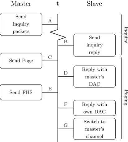
A number of preset steps need to be performed in order to set up a connection between two devices. First of all, the other device needs to be discovered. This is done by the inquiry process which hops through a specified subset of all frequencies to find the devices that are discoverable (figure 2.1 node A and B). It retrieves their 48-bits unique MAC address and the internal clock-offset. It
2.3. Inquiry process
f1 f2 f1 f2 f3 f4 f3 f4
Timeslot 1 Timeslot 2 Timeslot 3 Timeslot 4 Transmission Reception
Figure 2.2: Inquiry process per timeslot of inquirer
is exactly this process which is used in this research in depth and described in the next section.
After this discovery has completed, a paging procedure is started to actually set up a connection (figure 2.1 node C until G). The master device pages the slave device, which in return sends a reply containing its Device Access Code (DAC) on the appropriate frequency selected by the page response hopping sequence. The slave will then switch to the master’s channel parameters, by which a link is established and data can be exchanged. Most often this is done in the form of pairing. Pairs of devices negotiate a link key, a shared secret with which cryptographical authentication takes place. The stream of data may then be encrypted to prevent successful eavesdropping.
In order to communicate, Bluetooth uses a slow-hop frequency hopping spread spectrum scheme. This scheme consists of 79 frequency bands of 1MHz each, in the 2.4GHz range. In order to be incorporated into a Bluetoothpiconet
(a Bluetooth network), the device must be discovered in order to be able to exchange information to synchronize the hop sequence. Every piconet contains one master device, and up to seven active slaves. The master coordinates the transmissions of itself and its slaves by alternating in 625µs timeslots between master and slaves using time-division multiplexing.
2.3
Inquiry process
This research focuses on the behavior of Bluetooth devices during their inquiry process. As mentioned in the previous section, the inquiry process is designed to scan for other devices within range, and exchange the necessary information to set up an actual connection.
Bluetooth devices have two major states,connectionandstandby, and seven substates. Connection is used for communication whereas standby is the power-save mode in which no transmissions occur. The substates are used for joining as a slave in a piconet. Thepage substate is used by the master for adding slaves. For this paging procedure, the clock counter (28-bit, CLK) and the MAC address of the devices must be used. In the inquiry procedure this in-formation is exchanged in order to set up a lasting connection. As the master sends its address and clock value, the slave can construct the correct hopping sequence of the piconet by that information. The master also provides the slave with a 3-bit identification number. This limits the number of slaves in a piconet to seven.
2. Introduction to Bluetooth 11.25ms scan windo w 11.25ms scan windo w
Scan interval 1.28s Scan interval 1.28s
Figure 2.3: Scan windows per scan interval
11.25ms scan windo w 11.25ms scan windo w
Scan interval 1.28s 0-640ms
FHS sent
Backoff
Figure 2.4: Inquiry scanner behavior after FHS reply
inquiry substate, all communication in the piconet is put on hold. Therefore it is crucial to keep the inquiry window short. Another reason for keeping the inquiry window short is that it scans/transmits via a large subset of the Bluetooth frequencies, thereby interfering with other piconets that may be within range. Therefore the inquiry procedure is optimized to find all devices in the lowest amount of time possible. The master transmits inquiry packets on different frequencies (figure 2.1 node A). The slave, calledinquiry scanner, scans those frequencies at a slower rate, thus maximizing the probability of a correct reception.
An inquirer transmits two inquiry packets on two different frequencies dur-ing one regular transmission timeslot. 625µs later, the inquirer listens on the same fequency (figure 2.2). The inquiry scanners, in scan mode, change the fre-quency on which they listen every 1.28 seconds. In those 1.28 seconds they scan for 11.25 ms only (figure 2.3). After receiving an inquiry packet, the inquiry scanner replies with an FHS (Frequency Hopping Synchronization) packet 625 µs later (figure 2.1 node B), and enters a backoff period between 0 and 1024 timeslots (0-640ms, figure 2.4). This FHS packet contains the device’s address, its clock offset and a CRC code. Using this information a link can be estab-lished. This link is established by having the devices enter the paging substate, and go through the steps C until G of figure 2.1. This paging procedure is not important in this research, as the discovery is essentially complete at that time. We refer to [35] for more information on the paging procedure.
2.3. Inquiry process
The inquirer usesfrequency trains to determine on which frequency the in-quiry packets are transmitted. There are two frequency trains, A and B. At the start of the inquiry process, A and B both contain half of the 32 frequencies that are used. The inquirer then selects either A or B, and starts transmitting and scanning (figure 2.2) using that particular frequency sequence. After 1.28 seconds one frequency from both trains is swapped, so each contain one fre-quency of each other. The inquiry process then continues as normal. After 2.56 seconds, the entire train is swapped so that A becomes B and B becomes A. This means that after 2.56 seconds, the other 16 frequencies are used, enabling the inquirer to find the remaining devices that were not discovered earlier.
3
Bluetooth inquiry performance
Performance on itself is, just like Quality of Service (QoS), a term which re-quires a definition of which criteria are actually considered. In order to judge the inquiry process objectively, parameters of the inquiry process need to be defined which can be measured, monitored or derived. This chapter continues with defining the different parameters of the inquiry process. It also provides a way of judging these parameters to fit in the frame of the research on lo-calization as it is being done at Novay. After defining these parameters, their influence on the inquiry process is measured and their different effects have been described, each having their own section in this chapter. The contribu-tion of this chapter will be a conclusion as to how the discovery times change when multiple inquirers and inquiry scanners are used. The research question that will be answered in this chapter is
How do multiple inquirers influence the discovery time for each inquiry scanner
The experiments have been designed to answer this question accordingly.
3.1
Inquiry process parameters
The Bluetooth inquiry process, as described in the previous chapter, has many different variable parameters. These consist of user definable and tunable pa-rameters that control the process. In this particular order, the papa-rameters that are considered to be useful for this research have been described in the upcoming sections.
Dutycycle
3. Bluetooth inquiry performance
Scanning
Backoff
t= 0 t=a b < t < c
Figure 3.1: Dutycycle for (a,b,c) inquiry scan
the inquiry scanners can not be configured, the dutycycle is only accepted as a parameter for the inquirer.
The dutycycle can be specified by a series of three integers representing 1.28 second periods (see also figure 3.1):
(a, b, c)
where:
a. The periods the inquirer scans actively
b. The minimum number of periods of the dutycycle
c. The maximum number of periods of the dutycycle
This means that the backoff time is randomly chosen to end somewhere between b and c periods, leaving a minimum backoff period of b−a and a maximum backoff period ofc−a.
Example:
A dutycycle of (4,5,6) would scan for 4 periods, and backoff ran-domly somewhere between 1 and 2 periods.
The influence of the dutycycle is twofold. First of all it determines the ratio of the amount of time that is actually spent in scanning mode. Secondly it determines the intervals at which the random backoff time is introduced. The average ratio of the time spent in scanning mode versus idle mode can be calculated using an equation:
a (b−a)+(c−a)
2
(3.1)
which can be simplified in to:
2a
b+c−2a (3.2)
Example:
Suppose having a dutycycle of (4,5,6). This means the ratio of scanning versus idle time is
2·4 5 + 6−2·4 =
8 3
The interval at which the random backoff time is introduced is every a= 4 periods.
When having a lot of different inquirers this possibly influences the results of the inquiry process, which requires investigation.
3.1. Inquiry process parameters
Distance
[image:25.595.181.362.123.305.2]Signal strength
Figure 3.2: Distance versus perceived signal strength
Distance
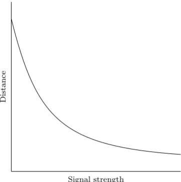
Distance is also a parameter of the inquiry process. The inquirers and scan-ners can be placed at a certain distance dfrom each other, creating a larger or smaller gap to be bridged by the transmissions. One could also consider placing the inquirers at different distances, and all variations that can be de-rived from this principle. The influence of this distance on the inquiry process can thus be determined by doing repetitive measurements while varyingd. It is already known that distance and perceived signal strength have a relation [17] (figure 3.2). The importance of the distance is therefore directly related to the localization problem. The effect of multipath fading and other signal distortion also have a relation with distance. This however can not easily be put in a graph as it relies heavily on environmental properties. A measurable influence of distance on the inquiry process therefore should exist. The results of this influence are discussed in section A.1.
Device type
Although Bluetooth devices are all built according to the same specification, there are several areas in which the manufacturer can make its own decisions. The specification also does not provide a detailed description of how a de-vice should be built, it merely lists the requirements which it should fulfill. This means the manufacturer is free to choose how he actually implements for example
• the antenna
• the casing
• transmission power
3. Bluetooth inquiry performance
These design choices influence the behavior of the system on all levels, in-cluding the inquiry process. Using different devices with, for example, different radio antennas, might reveal differences in the inquiry process. These however might be device related instead of particularly specific for the protocol itself. As the research goal is towards a practical localization system it is of interest how different devices behave. Nevertheless it needs to be kept in mind that obtained results can not simply be related to either the protocol or the device.
Power of transmission
The transmission power can be set in most devices. Manufacturers provide a required HCI [31] command set, which also provides support for getting and setting transmission power. As discussed in section 3.1 there is a relation between signal strength and distance. Changing the signal strength itself will therefore also be of influence. Multipath fading and other signal distorting influences also influence the perceived signal strength. Therefore there will also be a relation between these effects and the perceived signal strength.
Number of devices
The number of devices is also a parameter which can be changed. In a con-trolled environment this value can be explicitly selected. In field however, this value will be subject to constant change as people enter and leave transmission range. The effect of having multiple inquirers and inquiry scanners therefore is a parameter which is of great importance in this research.
When considering localization, the number of inquiry scanners represents the number of mobile devices that require localization. How many of those can be detected, and how fast, influences the performance of localization. The number of inquirers represent the number of access points that are used in a particular part of the localization area. Having more or less may influence how fast and complete the mobile devices can be detected.
As the number of inquiry frequencies is limited to 32, more inquirers will use up more of these frequencies. If the number of inquirers increases, the chance of collision between two or more will increase as well, thus influencing the results of the inquiry. Also, finding an inquiry scanner with multiple inquirers might be faster than with just one inquirer. These effects all determine the final shape of the inquiry process.
3.2
Experiment design
Designing the required experiments involves a few steps. First of all, the pa-rameters that are subject to the test need to be determined. As it is too extensive to test every possible combination of parameters, a selection of those should be made. The aim of the selection is to provide results from which most research questions (section 1.4) can be answered.
After making this selection, the location and setup of the experiment needs to be chosen. To minimize anything interfering with the data that is col-lected, this needs to be carefully done. How the events that occur are actu-ally recorded requires careful designing to minimize errors introduced during recording. When the recording of the data is completed, the data needs to
3.2. Experiment design
be processed in order to get the results which assist in answering the research questions. The recording process needs to be set up in such a way that pro-cessing the data can be done extensively, efficiently and correctly. Therefore, feedback after processing some initial measurements can assist in determining the final recording structure. The end of section 3.3 will discuss this.
Parameters
Of the parameters discussed in the previous section, a selection is made to use for the experiments. We have selected the parameters that are most likely to be of use in the area of localization. These are:
• dutycycle, because the amount of time spent scanning is important
• distance, because this is an important part of localization
• number of inquiring and inquiry scanning devices
The experiments for these parameters are split into two different groups. Before starting the actual experiment, the preferred dutycycle is established in a separate trial. When the dutycycle is selected, the experiments with distance and the number of devices can be conducted, using that particular dutycycle.
The remaining two parameters have not been selected as variable parame-ters in this research;
• Device type There are two reasons for not taking this variable into account. First of all a lot of different brands and types of devices are required in order to make a decent comparison. As the test should also be done with more than one device, it would be a logistical challenge to provide sufficient devices for the test. Secondly, it is very hard to draw conclusions from whatever results the experiments yield. The focus of the research lies on the real life behavior of the protocol during the inquiry process. The influence of different casings, antennas and transmission systems of all devices will make a comparison unreliable. The tests shall therefore be done using instances of one specific device type. Investigating if and how other devices behave differently is for future research.
• Transmission powerIt is generally possible to change the transmission power on Bluetooth devices. The HCI command set provides for the get-ting and setget-ting of such a value. On most mobile devices, this setget-ting is however not easily adjustable. Bluetooth dongles for PC-operation however are often equipped with a chip that supports this by easy con-figuration. It is a fair assumption that in the real world most devices will have the default transmission power setting. Usually this means maximum power for the Bluetooth class the device was built for. As the inquiry scanners in real world localization are mobile devices, their power setting is out of control of the system. During the experiments they will therefore not be changed. The power setting of the inquirers is also set to be fixed to limit the number of experiments.
3. Bluetooth inquiry performance
measurements, a selection of the distance/number of devices will be made and tested using different dutycycles. The results determine which dutycycle, if any in particular, is favorable. Table 3.1 contains the parameters with which the experiments have been done. Every combination of one value from each row makes for one individual experiment. Note that this adds up to 120 exper-iments. A single experiment will consist of the data of at least 100 executed dutycycles.
Dutycycles (2,3,4) (2,4,5) (6,7,8) (20,21,22)
Distances 2
Number of inquirers 1,2,3,4,5,7
Number of inquiry scanners 1,5,10,15,20
Table 3.1: Parameters for dutycycle experiments
The rest of the experiments use the preferred dutycycle, in combination with the parameters of table 3.2.
Dutycycles (a,b,c)
Distances 1,2,4,8,12
Number of inquirers 1,3,5,7
Number of inquiry scanners 1,5,10,15,20
Table 3.2: Parameters for other experiments
Note that this adds up to a total of 100 experiments, each consisting of the data of 250 executed dutycycles. This makes every experiment last for about 40 minutes (see section 3.3), leading to a total of 100·40 = 4000 minutes or 67 hours of collected data.
Choosing these specific distances, numbers of inquirers and numbers of inquiry scanners is done by consideration. The distances form a fair distribution on the maximum range of the used devices and their mobility. The number of inquirers is limited to seven for practical reasons. In a desired location-tracking system, having too many inquirers will increase the cost but probably not enhance the accuracy. As it is theoretically possible to track a 3d position with four devices, seven should at least suffice. As the used USB hubs have only seven output ports, seven is also a practical upper limit. When having one hub on the inquirer side of the setup, cable and hubs are left to spare for the inquiry scanner side, which is quantatively the most interesting side. On this inquiry scanner side, the maximum value is set to 20. There is no real theoretical reason for this particular upper bound. Practically speaking it is the largest amount of inquiry scanners the hardware can gracefully cope with when having three hubs.
Location and setup
Finding a suitable location to perform the experiments is not easy. The area needs to be as clear as possible from sources of interference, such as objects like furniture and interfering signals. At Novay, the souterrain basement (figure
3.2. Experiment design
Desk
Desk
PC
Inq sc.
Inq
Figure 3.3: Novay basement
3.3) proved to be empty. Thick concrete walls and a minimal amount of ob-jects occupying this space support a clean measuring environment. Signals can weakly penetrate this environment, like for example WLAN access points, but initial measurements however showed that Bluetooth signal penetration was very low. This most likely is the result of the larger signal strength WLAN uses by default. As the room is long, the experiments using maximum distance can still be performed by a clear line of sight between inquirers and inquiry scanners.
To perform the experiments, 4 USB hubs and two USB repeaters are used. Figure 3.4 shows the schematic design of this hardware setup. On one side, a USB hub is connected to the server. On the other side, two USB hubs are connected to the server, one of which is linked to yet another hub (figure 3.5). The capacity of each hub is 7 devices. On the inquirer side it is therefore possible to have up to 7 inquirers. On the other side it is possible to have 3·7−1 = 20 inquiry scanners. All devices that are put into the hubs are of the same type and have the same manufacturer: SiteCom, model no. CN-512 v2 001, with a Mavin Technology Inc (CSR 41B13) chipset.
Recording
Recording should be done in such a way that the recorded data can easily be processed to acquire the results. What actually is recorder is also subject of discussion, as the database should not get excessively large yet contain every bit of information that is useful in the research. Another aspect of recording is automation. As 67 hours of experiments have to be done, it is not desirable to have to do them by hand whilst changing the number of devices in the hubs every 40 minutes. A tool for recording and setting up the experiments automatically is therefore required.
3. Bluetooth inquiry performance
Inquiry scanners
Inquirers
[image:30.595.158.471.118.483.2]Figure 3.4: Experiment setup
Figure 3.5: Novay basement with inquiry scanners
is a console program which is hacked against the linux BlueZ [1] Bluetooth protocol stack. It allows Bluetooth devices to be put in inquiry mode with all parameters set correctly. It also makes it possible to shut down devices completely, to ensure that they do not create noise on the Bluetooth frequency band. The tool captures every FHS reply packet, and allows for its content to be stored directly to the MySQL database. We refer to section A.3 for an elaborate overview of this tool. A Linux shell script is used to invoke the tool, using different commandline parameters which control the parameters of the experiment that is performed.
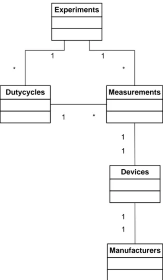
The recorded data is placed into a single database-table named ”measure-ments”. Figure 3.6 shows how the different tables that are used interact. Every table serves another purpose:
• Experiments For every experiment, this table records the parameters of the experiment, and a time of start and end.
• Dutycycles For every dutycycle of each inquirer in the experiment, its
3.2. Experiment design
Experiments
Measurements
Devices Dutycycles
Manufacturers
1 *
1 *
1 * 1 1
[image:31.595.188.352.125.405.2]1 1
Figure 3.6: MySQL table structure
time of start and end is recorded. This way it will be possible to calculate at which time relatively to the dutycycle the event occurred.
• MeasurementsFor every FHS that is returned by an inquiry scanner, the data package is stored in this table. This includes the RSSI value, and exact timing information timestamped by the server when the FHS arrives.
• Devices This table contains a list of all devices that are used in the test. It serves as a DNS for translation the text labels which have been attached to the devices, to their MAC addresses. If an unknown device is discovered during a test, it is added to this list with an empty label.
3. Bluetooth inquiry performance
Processing results
Because the data is collected into a database, well designed database queries can make processing the results a lot easier. It needs to be kept in mind that processing the results should ideally be done in a short amount of time. Queries that take several minutes to complete make the analysis slow, and tweaking the process itself tedious. As the ’measurement’-table will contain a few million entries, this definitely requires consideration.
To make the results of the different experiments easily accessible and un-derstandable, a series of web pages have been developed. These web pages list all experiments, and provide automatically generated graphs and statis-tical information for each experiment. Dynamically combining results from different experiments however is not possible, and should be done by hand or programming. Section A.3 shows the features and design of this web service, and presents the overview of all experiments. Using the framework built for that service, other information can be extracted more easily from the database and presented to the user accordingly.
Dutycycles and Observation Windows
There is one particular thing about the interpretation of the word dutycycle
during the processing of the results that requires explanation. When several inquirers are involved in an experiment, each inquirer has its own dutycycle. As the backoff period is random for each inquirer, dutycycles itself are not syn-chronized. It would therefore make no sense to analyze the data of the different inquirers together, on a per dutycycle basis. In the field, when localizing and discovering new devices, a measurement starts at a certain moment. At that moment, it can not be predicted in which time and phase of the dutycycle the device currently is. A global ”dutycycle”, henceforth called ”observation win-dow”, can therefore be introduced to counter that problem. Figure 3.7 shows how this can be achieved. As all inquirers have their own dutycycle, an obser-vation window is introduced covering both the active and non active phase of the dutycycles. This observation window has no backoff time, as they are auto-matically included. Basically it comes down to congregating the measurements of all inquirers and analyzing them in predetermined intervals which are then called observation windows. Because all backoff times of the inquirers can be seen as random after some time, the global view will be valid. In terms of prac-tical approach, this simulates the real world in the following way; devices enter and leave the vicinity of the monitored area. The inquirers are inquiring, all in different stages of their respective dutycycles. One of the questions is: how fast will they discover. To derive the distributions of such events, the data will be analyzed starting at some point in time, taking all incoming measurements from that time on, into account. This is what figure 3.7 represents.
3.3
Effect of dutycycles
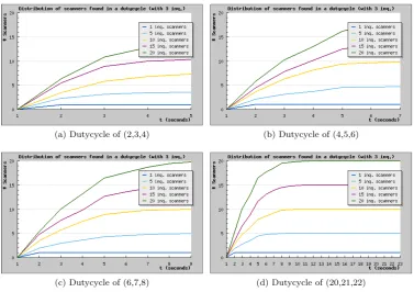
Figure 3.8 shows four of the 24 graphs of the conducted experiments. The graphs show the average time that is needed for 3 inquirers to discover the various number of inquiry scanners within each ordinary dutycycle. Note that the data is aggregated over the three inquirers, and that the x-axis contains
3.3. Effect of dutycycles
timet
Observ. window Inquirerc
Inquirerb
Inquirera
Figure 3.7: Congregation of dutycycles to ”observation window”
c+ 1 seconds. The aggregation is done by mapping all dutycycles in one graph and derive the average. Because the data from the experiments also contains the start of all dutycycles for each inquirer, the timing for each inquirer can be very accurately shown.
Example:
The green line in figure 3.8c represents an experiment with 20 in-quiry scanners. As can be seen in the title of the graph, 3 inquirers were simultaneously used at that experiment. After 2 seconds in the observation window, on average 5 devices were discovered. Af-ter 5 seconds in the observation window, on average 16.5 devices were found.
For determining the final dutycycle there are three criteria. On one hand the dutycycle must be short in order to maximize the amount of randomness created by the backoff period. On the other hand the dutycycle must be long enough to allow a maximum amount of discovery before the inquirer enters the backoff period. Also the dutycycle should have a small idle time to maximize efficiency. The dutycycle (2,3,4), for example, has an active scanning part of 2 periods, followed by on average 1.5 idle periods. This means that efficiency is low. The graphs show that there is little difference in the amount of devices that are discovered at a particular timet for different dutycycles. One exception is figure 3.8a, which discovers significantly less devices at t= 5. This dutycycle implies that only 2·1.28 = 2.56 seconds are actually spent in scanning mode. This means that it is possible that not all frequency trains have been covered by the inquirers, which results in a loss of overall discovery.
Not having large deviations in the measurements is an informal measure for the quality of the measurements. The time spent in scanning mode should theoretically not determine the number of devices that are found within a certain timet. The graphs clearly show that this is indeed the case.
3. Bluetooth inquiry performance
(a) Dutycycle of (2,3,4) (b) Dutycycle of (4,5,6)
(c) Dutycycle of (6,7,8) (d) Dutycycle of (20,21,22)
[image:34.595.155.533.163.429.2]Figure 3.8: Time to discovery of inq. scanners, for different dutycycles
Figure 3.9: Figure 3.8c expressed in percentages
3.4. Effect of multiple devices
Figure 3.10: Figure 3.9 interpreted using a 6000ms observation window
(a) 15 inq. scanners at 2m (b) 20 inq. scanners at 4m
Figure 3.11: Time to discovery of inq. scanners, for different number of inquir-ers
Although the (6,7,8) dutycycle is selected based on clear information and graphs, determining the dutycycle for which to carry out the experiments is not that easy. This is due to the different nature in which the dutycycles are interpreted in the other experiments (section 3.2), referred to as observation window. To verify the selected dutycycle, figure 3.9 is converted into an obser-vation window interpretation (figure 3.10). An obserobser-vation window of 6000ms is used instead of the individual dutycycles of the inquirers. It can be seen that the regular discovery percentage at 6s is exceeded. In fact, close to 100% is already achieved at thet= 3500ms mark. Besides showing other interesting behavior (see section 3.4), this means that the (6,7,8) dutycycle in combina-tion with the 6s observacombina-tion window is appropriate for the situacombina-tion. They will therefore be used in the remaining part of this research.
3.4
Effect of multiple devices
3. Bluetooth inquiry performance
(a) 3 inquirers at 2m (b) 5 inquirers at 4m
Figure 3.12: Time to discovery of different amounts of inq. scanners
(a) 3 inquirers at 2m (b) 5 inquirers at 4m
Figure 3.13: Time to discovery of different amounts of inq. scanners, in per-centages
Effect of multiple inquirers
Figure 3.11 shows the general results of the experiments for a different number of inquirers. Note that from this moment on, observation windows are used instead of dutycycles.
Example:
Observe the purple line of figure A.2a. This line shows the accumu-lated percentage of inquiry scanners that are discovered over time, by seven inquirers. For example, after t = 1000ms around 75% of the 15 inquiry scanners is discovered.
The figures show that having one inquirer itself has a low discovery rate. From 3 inquirers on, the rates become stabilized. Note that there are no measurements for two inquirers, leaving the gap between the one and three inquirer graphs unfilled. It can therefore not be concluded if the two-inquirers graph would lean more towards the one-inquirer or the three-inquirer graph.
3.5. Related work
(a) 3 inquirers and 10 inquiry scanners (b) 5 inquirers and 15 inquiry scanners
Figure 3.14: Time to discovery at different distances, in percentages
Effect of multiple inquiry scanners
Figure 3.12 shows the general results of the experiment with different amounts of inquiry scanners. Observe that having more inquiry scanners results in a better discovery of individual inquiry scanners. Figure 3.13 shows the same graph except the percentage of discovered devices is plotted. Introducing the observation window has introduced a behavior that we did not find in any literature. Apparently it does not matter how many inquiry scanners there are present, after a specific timetthe same percentage of devices is discovered. All 20 of the generated graphs show exactly this same behavior. At first sight it may seem awkward, but section 3.6 will show that the measurements themselves are valid. Also the way in which the graphs are derived from the data has been thoroughly reviewed, and found to be correct.
We have not found this behavior documented in other research for version 1.2, therefore making this an interesting contribution to the general Bluetooth discovery research.
Statement:
With an arbitrary number of inquiring devices, between a certain timetandt+ ∆t, the same percentage of discoverable inquiry scan-ners within range is discovered. Provided the distance of the inquir-ers and the inquiry scanninquir-ers is the same and the same conditions apply.
This can be used for predicting the total number of scanners, given the number of found scanners in a period. The conclusion of the effect of multi-ple inquiry scanners is therefore easily drawn and can be summarized in the statement above.
3.5
Related work
3. Bluetooth inquiry performance
having multiple inquirers, and the time in which the inquiry scanners are de-tected by at least one of these inquirers. When trying to improve the discovery protocol for communication, such an approach makes perfect sense. When the discovery is only used for aiding localization this is of no major importance. [26] and [10] are examples of papers that contain simulation results for one inquirer only. In [26] the same definition of a discovery is used; the time to receive and FHS packet from the inquiry scanner. After explaining the working principles of Bluetooth, they derive the timing information from the inquiry process. From this information, probabilistic information is extracted as to the hit and mis ratio of the frequency hopping of the FHS packets of the inquiry process. Although the paper is called ”Bluetooth Discovery Time with Mul-tiple Inquirers”, they unfortunately conclude that an analytical model is not feasible, and ”although the single inquiring device inquiry time has been well characterized, the effect of multiple inquirers is difficult to model and has not been considered”. However, they do present a table containing the inquiry time with multiple inquirers, constructed by a simplified model in Matlab. This sim-ulation models a single scanning node over a perfect channel in the presence of multiple inquirers. This results in a table with mean inquiry times for 1..5 in-quirers. The value of 1.80sfor 1 inquirer matches the results from this research, however the other values do not. Due to a different interpretation of discovery, the discovery times of the paper are significantly higher when compared to our discovery times, as they measure the time to have an inquiry scanner detected by each inquiry scanner instead of just one. Because we are interested in lo-calization, we do not care which inquirer detects a device. Unfortunately this paper uses Bluetooth version 1.1. [10] is limited to a simulation for multiple inquiry scanners. After extensive analysis of the discovery protocol a simulator has been written using the original Bluetooth frequency train obtained from the specification. Although we have plenty of measurements of 1 inquirer with multiple inquiry scanners, the results can again not be compared. Whereas in the paper the inquirer has to find all inquiry scanners, we stop at the first inquiry scanner discovered. The results for 1 inquirer and 1 inquiry scanner however do match. In the paper they simulated an average discovery time of 1.5sin ideal circumstances, whereas we found it to be 1.8sin practice.
There is a reason why the values of this research can not be compared with Bluetooth version 1.1 reliably (as seen in [24] and [26]). In version 1.1, the inquiry scanner enters a backoff time after receiving the FHS. After that, a second discovery must take place by exactly the same inquirer, before the device is actually considered to be discovered. Due to this backoff time and same-inquirer requirement, the device is unable to be discovered by other same-inquirers for a considerable amount of time ([24]). In essence this leads to a larger mean discovery time when multiple inquirers are used on only one inquiry scanner. This is not the case in version 1.2, which requires only one discovery instead of two. In version 1.2, having multiple inquirers would not reduce the average discovery time, yet increase it. When comparing the values for only one inquiry scanner this effect is small, but when multiple inquiry scanners are used, the values can not be compared reliably.
In [24] a different approach is taken. An analysis is performed to obtain optimal parameters for the discovery phase thus proving that the default values are not optimal. A table is present showing the percentage of not-discovered devices, including the average discovery time. Although the paper uses
3.5. Related work
tooth 1.1 instead of 1.2, the value for one inquirer and one inquiry scanner can be used as a reference. For one inquirer and one inquiry scanner, 1.91 seconds is required on average to find a device. Although the distance between scanner and inquirer is not given, the average measurement we derive using version 1.2 with our observation window is 1.8 seconds.
In [16] a formal analysis made of the Bluetooth discovery protocol. This is done for version 1.1 as well as version 1.2. After an extensive discussion of the workings of the protocol, a probabilistic model is introduced. This model is based on the different aspects of the discovery phase. The extent in which the probabilistic part of the model checking is used is relatively small. Instead of using the absolute timing values, they are transformed to probabilities, so if a device is generally discovered inntimeslots with an even distribution, the chance of discovery in a timeslot is n1. By using this approach, the influence of probabilistic modelling versus regular modelling is not large. The discovery procedure is broken down into a set of discrete time Markov chains (DTMCs). A setup for the probabilistic model checker PRISM is then introduced. The model is only used to calculate the values for one inquirer and one inquiry scanner. It is just this value that can be compared to our research. The simulation shows an even distribution of probabilities from 1.92sto 1.93swhich therefore relates to our findings in the same way as the previously discussed papers do.
[9] is a paper on the the analysis of discovery and delay of Bluetooth de-vices. The aim is to provide an alternative backoff-time which lowers the overall discovery time yet preserves and respects the intentions of the back-off time. A bluetooth simulator has been written to simulate the behavior for different values for the number of backoff slots. Pracitcal measurements have also been done, but these are only mentioned to be in accordance with the values of the simulation. For the standard value of 512 backoff slots, the derived discovery time is 1.4sfor one inquirer and one inquiry scanner. Although more inquiry scanners are used, their values can again not be compared. This paper con-cludes that the number of backoff slots proposed in the standard is too high. Equally good results can be obtained by reducing the number of backoff cycles to half its original amount, proposedly 200-300 (5122 ).
3. Bluetooth inquiry performance
6.2s, whereas our experiments show that it is possible to achieve the same dis-covery in 4.6 seconds. As the simulation is always more optimistic than the experiment, this figure will show a larger deviation in practice. In short, the behavior shows characteristics that confirm the behavior we discovered, but due to a difference in Bluetooth versions can not be compared in detail.
3.6
Discussion
How reliable the obtained results are depends on several factors:
• EnvironmentChanges in the environment, for example a moved object, can result in a difference in signal reception.
• ClimateChanging humidity and temperature affect wireless signal trans-missions.
• Interference Other radio-sources may interfere with the signals of the experiment.
• Test setupMoving test devices or placing them in an awkward position influences the way in which the transmissions perform.
• Data collection If for example measurement resolutions are very low, or if there are buffers that can get overflowed when not polling correctly the data collection can become unreliable.
• Data AnalysisIf the analysis is performed incorrectly data can be mis-interpreted and result in conclusions that do not reflect the actual data.
The environment has not been subject to any physical change during the experiments. Furthermore, most of the influence of environment, climate and interference would have to be visible in the RSSI values of the measurements. It can be seen in the measurements that no significant changes in RSSI have occurred where they are not to be expected. This indicates that the influence of climate and interference was relatively low, although the experiments took several weeks to complete.
The test setup is easy, and does not show any signs for concern about the validity of the measurements it produces. Although the individual devices are relatively close to each other, this should based on the frequency hopping not be a problem. The vertical placement of the devices does require attention. During initial testing is was discovered that performance of the system was considerably worse if all devices were placed directly onto the floor. Probably an excess of relay scattering resulted in poor performance. Placing the devices about 1.5 meters of the ground proved to increase performance. Due to the concrete isolation of the room, signal penetration was low. In combination with the results of [20] this makes intereference an unlikely source of problems.
The data collection is partially discussed in section A.3, and should not in-fluence the measurements too much. This is however a misleading assumption, as the subsection on FHS delays discusses later.
The data analysis is, on a high level, discussed in section A.3. Several of the data-analysis scripts have been externally reviewed by colleagues to ensure proper design and implementation. Especially the scripts that generated the
3.6. Discussion
(a) Distance of 1m (b) Distance of 4m
Figure 3.15: FHS packets per dutycycle
Figure 3.16: Simulated probability density for inquiry scan from [22]
graphs of section 3.4 have been subject to this review.
FHS packets
A more analytical approach to testing the reliability of the results can be per-formed using the actual low level measurements. During most of the analysis, only the first FHS packet of each inquiry scanner was used. As the discovery of a device depends upon the time at which this first packet is received, other packets received by this inquiry scanner in the same observation window are of no importance. When analyzing if the inquirers actually receive data in a way that can be matched to the theoretical approach of the Bluetooth protocol, these packets do have their use.
3. Bluetooth inquiry performance
A Bluetooth inquirer changes one frequency of the frequency train every 1.28 seconds (section 2.3). After 2.56 seconds the entire frequency chain is changed to contain all frequencies that were not present in the train of the first 2.56 seconds. The graphs show that the incoming FHS packet behavior is according to what should have been suspected when regarding the protocol. The first 1.28 seconds a lot of devices are found. The second 1.28 seconds only one frequency is changed in the train, thereby only changing by 1
32. The influence of this on receiving FHS packets is small. After the 2.56 seconds, the entire frequency train changes allowing for almost all remaining inquiry scanners to be detected. The graph clearly shows a new batch of packets from inquiry scanners being received from that moment on. Figure 3.16 shows a simulation of the inquiry scan from [22]. This graph shows exactly the same behavior as the graph in figure 3.15.
FHS delays
For this approach the time between successive FHS packets from the point of view of the inquiry-scanners is taken. In other words, for every inquiry scanner, its ∆ FHS is observed. Figure 3.17 (equals figure 2.4) shows the behavior of the inquiry scanner between successive FHS replies. After an FHS packet is sent, the inquiry scanner enters a maximum backoff period of 640ms. Immediately after this backoff time another scan window is opened. Therefore, another FHS can be discovered in the scan window immediately after the backoff, or k·1.28slater. Using this theoretical insight, the reliability of the data can be determined.
Example:
• If the backoff time was 0ms, the first scan window after the backoff time is immediately. The next one is then after 1.28 seconds.
• If the backoff time was 640ms, the first scan window after the backoff time is after 640ms. The next one is then after 1.92 seconds.
If we consider all ∆ FHS times lower than 1.2 seconds, this means that only the cases are considered in which the second FHS was received in the first scan window after the backoff time. These ∆ FHS times should be lower than 640 + 11.25ms, because after that there is no scan window to receive them anymore. When the ∆ exceeds this 651.25ms, this means that there was some form of a delay between the arrival of the FHS and its actual timestamp. This delay can happen when the Bluetooth chip reports the FHS later than it has actually arrived, or when there has been a delay between the chip reporting the FHS and its actual timestamping by the software of the measuring equipment. Figure 3.18 shows the ∆ FHS times that are lower than 1.2 seconds. This figure shows that there are still packets timestamped after the 651.25ms mark, which ideally should not happen. This means that there is indeed a delay which occurs between FHS reception and its timestamp. Why this delay exactly occurs is very hard to determine. Although the tool that is used for timestamping the packets uses polling to acquire the messages from the Bluetooth devices, this does not introduce a significant delay by itself. In worst case there are only
3.6. Discussion
11.25ms scan
windo w
11.25ms scan
windo w
Scan interval 1.28s 0-640ms
FHS sent
Backoff
Figure 3.17: Inquiry scanner behavior after FHS reply
Figure 3.18: FHS Delay
7 inquirers that require polling. Therefore, the delay must be also present in either the used Bluetooth device, or the handling of Bluetooth packets by the USB hardware of the PC or the Operating System. In [28] it is suggested that messages may be delayed significantly when the device is busy:
Unfortunately, the reply from the Bluetooth module may be signifi-cantly delayed if the Bluetooth module has received a data message via radio and is sending this message to the main processor ..., such that the communication channel (”Bluetooth-to-MCU channel”) is blocked.
Although this will account for a small amount of errors, there still is the issue of multiple inquirers increasing the delay. This suggests that the USB hardware or the Operating System is most likely to be the major cause of this effect.
3. Bluetooth inquiry performance
Inquirer
Inquirer Application
D ela
y C
Del ay A
Delay B Inquirer
Figure 3.19: Delays between inquirers and application
In addition to that, the Host Controller (PC) directs traffic flow to the devices, which means that devices can only transfer data on the bus with an explicit request from the Host Controller. In USB 2.0 this is done by querying the connected devices, usually using a round-robin scheduling algorithm [38]. The PC, in this case, has a maximum of over thirty devices that require polling. Where the delay exactly occurs is, as discussed, hard to determine. In chapter 4 a new experiment is suggested which removes the currently suspected causes of the delay.
The implication of these delays is that it is not possible to compare timing aspects of experiments with a different number of inquirers, as the number of inquirers show to influence the delay. Figure 3.19 shows the delays as they occur for each inquirer. Between the application and each inquirer a delay occurs. If it is assumed that the delay is on average a constant for every individual inquirer, the data for each inquirer is valid. If this is the case, delay {A,B,C} are not equal, and a time critical comparison between the results of these devices can not be made.
Therefore the results of this chapter are still valid:
• Effect of dutycycles This part does not compare different numbers of inquirers in a time critical way. It is based on how many devices are discovered in a certain dutycycle, which is not influenced by delay. Although the timestamp may be later, the actual dutycycle number in which the device was discovered still is valid.
• Effect of multiple devicesThe effect of multiple inquirers is based on observation windows instead of duty cycles. These rely on the timestamps of the FHS packets, and congregate the data of the entire experiment. If short and longer delays are experienced, they will even out to an average delay which is the same for experiments that have the same amount of inquirers. No conclusions based on data from experiments with a differ-ent number of inquirers have been made. The same holds for the effect of multiple inquiry scanners. The analysis is based on the observation windows, in which only the average delay is a factor. As the data is not compared to the data of experiments with a different number of inquirers in a time critical way, the conclusions are still valid.
3.7. Conclusion
Discovery time Backoff time
FHS interval F FHS sent
B D
FHS sent
Figure 3.20: Inquiry scanner FHS Interval labelling
• Effect of distance The effect of distance is determined based on two different factors. The same experiments are repeated using different dis-tances. As the delays of the timestamps can in that case be considered equal, the difference between the experiments at different distances is valid. For the second part, the research is based on the RSSI value of the measurements, not on the timing information of the measurements. Therefore delays do not influence the result.
As chapter 4 will require a detailed comparison of discovery times among experiments with different numbers of inquirers, the specific experiments for that chapter have been redone using a different approach (section 4.2.1).
3.7
Conclusion
4
Modeling discoveries
This chapter is aimed towards creating a simple but functional model of the actual inquiry process. Formal models