doi:10.4236/jbise.2011.49073 Published Online September 2011 (http://www.SciRP.org/journal/jbise/).
Generalized electro-biothermo-fluidic and dynamical
modeling of cancer growth: state-feedback controlled
cesium therapy approach
Murad Al-Shibli
College Requirement Unit, Abu Dhabi Polytechnic, Institute of Applied Technology, Abu Dhabi, United Arab Emirates. Email: [email protected]
Received 21 December 2010; revised 23 February 2011; accepted 5 July 2011.
ABSTRACT
This paper develops a generalized dynamical model to describe the interactive dynamics between normal cells, tumor cells, immune cells, drug therapy, elec-tromagnetic field of the human cells, extracellular heat and fluid transfer, and intercellular fractional mass of Oxygen, cell acidity and Pancreatin enzyme. The overall dynamics stability, controllability and observability have been investigated. Moreover, Ce-sium therapy is considered as a control input to the 11-dimensional dynamics using state-feedback con-trolled system and pole placement technique. This approach is found to be effective in driving the de-sired rate of tumor cell kill and converging the sys-tem to healthy equilibrium state. Furthermore, the ranges of the system dynamics parameters which lead to instability and growth of tumor cells have been identified. Finally, simulation results are demonstrated to verify the effectiveness of the ap-plied approach which can be implemented success-fully to cancer patients.
Keywords:Cancer; Tumor Growth; Tumor Dynamics and Modeling; Immune System; Cesium Therapy; State-Feedback Control; Pole Placement
1. INTRODUCTION
There are over 200 different types of cancer that affect virtually every organ in the body. They can seem bewil-deringly different but all cancers share certain features as outlined by Douglas Hanahan and Robert Weinberg [1]. Six essential alterations in cell physiology that collec-tively dictate malignant growth: self-sufficiency in growth signals, insensitivity to antigrowth signals, eva-sion of programmed cell death (apoptosis), limitless rep-licative potential, sustained angiogenesis, and tissue in-vasion and metastasi.
The technical report [2] presents what is known today concerning non-ionizing electromagnetic field interac-tion with the human body. Many significant and inter-esting effects are identified. As an example, both theo-ries and observations link non-ionizing electromagnetic field to cancer in humans, in at least three different ways: as a cause, as a means of detection and as an effective treatment.
A phase-space analysis of a mathematical model of tumor growth with an immune response and chemother-apy is introduced in [3]. It is proved that all orbits and trajectories are bounded and converge to one of several possible equilibrium points. The addition of a drug to the system can move the solution trajectory into a desirable basin of attraction.
State Dependent Riccati Equation (SDRE) based op-timal control technique to a nonlinear tumor growth model is applied in [4]. The model consists of three bio-logical cells which are normal tissue, tumor and immune cells. The effect of chemotherapy treatment is also in-cluded in the model. Chemotherapy administration is considered as a control input to the nonlinear cancer dynamics and the amount of administered drug is deter-mined by using SDRE optimal control. The optimal con-trol is applied to the model in order not only to drive the tumor cells to the healthy equilibrium state but also to minimize the amount of the drug used.
A basic mathematical model of the immune response when cancer cells are recognized is proposed. The model consists of six ordinary differential equations [5]. It is extended by taking into account two types of therapy: active immunotherapy and adoptive immuno-therapy. An analysis of the corresponding models is made to answer the question which of the presented methods of immunotherapy is better.
models of solid tumour growth may yield. These range from discriminating between competing hypotheses for the formation of collagenous capsules associated with benign tumours to predicting the most likely stimulus for protease production in early breast cancer.
Understanding the dynamics of human hosts and tu-mors is of critical importance [7]. A mathematical model was developed that explored the immune response to tumors that was used to study a special type of treatment. This treatment approach uses elements of the host to boost its immune response in the hopes that the host can clear the tumor.
Two models of optimizing tumor growth are presented in [8] In the first model optimal controls minimize the tumor volume for a given amount of angiogenic inhibi-tors to be administered while the second formulation tries to achieve a balance between tumor reduction and total amount of angiogenic inhibitors given. For both models a full synthesis of optimal solutions determined by portions of bang and singular controls with rest peri-ods is presented. The differences in the two solutions are discussed.
A new mathematical model is developed for the dy-namics between tumor cells, normal cells, immune cells, chemotherapy drug concentration and drug toxicity [9]. Then, the theorem of Lyapunov stability is applied to design treatment strategies for drug protocols that ensure a desired rate of tumor cell kill and push the system to the area with smaller tumor cells.
Cells, whether cancerous or normal can only live and reproduce (undergo mitosis) in a pH range of between 6.5 and 7.5. A healthy cell has a pH of 7.35 while a can-cer cell is more acidic. When the pH of a cancan-cer cell goes above 7.5 it dies and if it goes above 8.0 it will die in a matter of hours.
Every cell in the body works as milli-volt battery. To successfully bring nourishment in, and take poisons out, it has to be fully charged. In a cancerous cell, the cell voltage drops from 90 millivolts to less than 40 milli-volts. When the cell voltage gets to the very bottom, only 5 substances can pass in or out of the cell. They are water, sugar, potassium, cesium and rubidium. Oxygen cannot enter into a cancer cell. Even if there is a lot of oxygen in the blood, it won’t get into the cell.
Potassium ions are responsible for the ability of glu-cose to enter the cell. Potassium enters cancer cells in a normal manner so glucose still enters the cancer cell. Cancer cells have only 1% of the calcium content found in normal healthy cells. The calcium, magnesium and sodium ions, which are responsible for the intake of ox-ygen into the cell, cannot enter the cancer cell but the potassium ion still enters these cells. Thus we have can-cer cells containing glucose but no oxygen.
A healthy individual has a blood oxygen level of be-tween 98 and 100 as measured by a pulse oximeter. No-bel Prize Laureate, Dr. Otto Warburg, discovered that when he lowered the oxygen levels of tissues by 35 % for 48 hours normal cells were converted into irreversi-ble cancer cells [10]. Cancer patients have low levels of oxygen in their blood usually around 60 compared to normal values of about 100 by pulse oximetry. The common therapies used to treat cancer (chemotherapy and radiation) both cause drastic falls in the body's oxy-gen levels. Tissues that are acidotic contain low levels of oxygen whereas tissues that are alkalotic have high lev-els of oxygen.
When oxygen fails to enter the cell the cell's ability to control, its pH is lost and the cell becomes quite acidic. This is caused by the appearance of abnormal metabo-lism (anerobic glycolysis) in which glucose is converted (fermentation) into two particles of lactic acid. This production of lactic acid promptly lowers the ph within the cell to 6.5 or lower. The lactic acid damages the tem-plate for proper DNA formation. Messenger RNA is also changed so the ability of the cell to control its growth is lacking. Rapid and uncontrolled cancer cell growth and division occurs. Vitamin C and zinc are able to enhance the uptake of cesium, rubidium, and potassium into can-cer cells.
Cancer cells develop a protein coating 13 times thick-er than normal cells. This makes it difficult for the im-mune system to attack them. By ingesting high doses of pancreatin, you can actually dissolve cancer cells inside the body [11]. In the natural course of one’s life-time, millions of cancer cells develop, and are harmless-ly digested by the immune system. The body uses pan-creatin, a secretion from the pancreas to dissolve the cancer cells. As we age, the pancreas is less and less able to make this important substance. By taking pancreatin orally, it is possible to increase the levels of its active ingredients in the blood, thereby helping the body break down the cancer cells and remove them from circulation. The active ingredients in pancreatin which have shown to have tumor dissolving abilities are trypsin and chy-motrypsin. These ingredients were taken out of virtually all the pancreatin supplements available to consumers years ago. These active ingredients are being bought in massive quantities by the sewerage industries to digest the sewerage into less noxious forms.
out a convenient way for the administration of the ther-apy. These experiments, in general, take a long time and most importantly may result in many deaths during the development period. Clinical experiments also reveal the fact that there is a strong relationship between the cancer state (the number and/or volume of tumor cells, tumor type), the immune system of the patient and the treat-ment strategy. Hence, understanding the dynamical be-havior of cancer has received a great interest.
This paper develops a generalized dynamical model to describe the interactive dynamics between normal cells, tumor cells, immune cells, drug therapy, electromagnetic field of the human cell, extracellular heat and fluid transfer, and intercellular fractional mass of oxygen, cell acidity and pancreatin. The overall dynamics stability and controllability has been investigated. Moreover, Ce-sium therapy is considered as a control input to the 11-dimensional dynamics using state-feedback con-trolled system and pole placement technique. This ap-proach is found to be effective in driving the desired rate of tumor cell kill and converging the system to healthy equilibrium state. Furthermore, the ranges of the system dynamics parameters which lead to instability and growth of tumor cells have been identified. Finally, sim-ulation results are demonstrated to verify the effective-ness of the applied approach which can be implemented for each individual case.
This paper is organized as follows. Section 2 intro-duces modeling of the electromagnetic field of a live cell, cellular heat and fluid transfer are presented in Sections 3 and 4, respectively. Cellular factional composition is outlined in Section 5, generalized cellular-tumor dy-namics is detailed in Section 6. Controllability and state-feedback control design of tumor dynamics are presented in Section 7. Section 8 demonstrates simula-tion which followed finally conclusions.
2. ELECTROMAGNETIC CELLULAR
MODELING
A great variety of theories have been developed to de-scribe the electro-magnetic field of the human body. Some theories regarded the human body as a whole as single prolate spheroid with a single set of electromag-netic constants: permittivity, permeability, and conduc-tivity [2].
In that sense, the body is a simple antenna or probe capable o f intercepting a certain amount of electromag-netic energy, which is converted entirely in to heat. At the other extreme, the body may be regarded as a collec-tion of countless electronic microcircuits, each one cor-responding to an individual cell or partially. Electro-magnetic energy somehow finds its way to individual microcircuits and influences the electronic functions
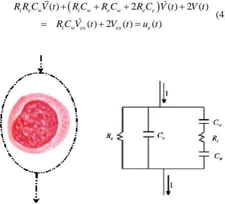
there. These functions include various communication and control processes essential to life and its activities. Efforts to understand these have focused attention on the microscopic components of the tissues such cells, mem-branes, fluids, molecules in solution rather than the tis-sue taken as a whole. Some theories have been devel-oped concerning individual cells. An equivalent circuit has been developed as shown below. Given an incident current or current density actually passing across the cell membrane through and through the cell can be calculat-ed. If the current is sufficiently enough, different re-sponses are possible. For example a current density of 1 mA/cm2 is about the amount associated with the action potential of nerve and muscle cells. Perhaps a pulsed electromagnetic filed could simulate these action poten-tials and confuse the body by generating false signals.
Of the cells part, the membrane probably has attracted most attention at least with respect top electromagnetic effects. Many membrane properties have been quantified. Typical thickness 45 Ang, typical capacitance 1 micro-farad/cm2, typical leakage conductance 1 - 10 mhos/cm2, typical resting potential 100 millivolts, dielectric con-stant 5, Electric field 22 Million V/m, Surface charge density 9.7 × e–8 C/cm2 = 6.1 × e11 charge/cm2. Of these perhaps the electric filed is the most remarkable one since it is almost greater than any other found in nature. For example the electric field of the Earth at its surface is only about 100 V/m.
So far the membrane has been treated as a homoge-nous substance and characterized by a capacitance and nonlinear conductance. In fact the membrane is not ho-mogenous. The basic structure is a double layer of mol-ecules called lipids. Lipids are hydrophobic, that is, they repel water. It is the repulsion that holds the membrane together. Proteins are chains of mino-acids. Proteins are so important because they can conduct charges while lipids are good insulators. Thus proteins are the con-ductance in the electronic circuit of the membrane.
Electromagnetic field can interact with proteins over a wide range of frequencies between 1 - 10 MHz. It de-pends on its size and mass protein can be modeled as single dipole which rotates in response to an oscillating field.
enough cells to form a tumor which characterized by poorly circulated system. So, little or no oxygen-carrying blood reaches the cells.
The equivalent impedance (resistance) Zeq of the equivalent electric circuit of the human cell can now be expressed in the Laplace domain as:
2
2
2 2
i e w e
eq
i e w i w e w e e
R R C s R Z
R R C s R C R C R C s
(1)
where Ri is the intracellular medium resistance, Re is the extracellular medium resistance, Cw is the capaci-tance of the cell wall, Ce is the capacitance of extra-cellular medium.
Now it is possible to express the voltage across the cell V s( ) using Ohm’s law such that
( )
( ) eq
V s Z
I s (2)
where the I s( ) is the passing cellular current.
The voltage-current time change can be formulated by taking the Laplace inverse of the former equation as fol-lows (assuming zero initial conditions)
( ) 2 ( ) 2 ( )
( ) 2 ( )
i e w i w e w e e
i e w e
R R C V t R C R C R C V t V t
R R C I t R I t
(3)
The right hand side of the last Eq.3 represents the in-put source to the cell. Since Re represents the extra-cellular resistance then the term R I te ( )V te( ) is the external voltage source to the cell and the term
( ) ( )
e ex
R I t V t the rate of change of the external voltage source. The equation now can be modified to
( ) 2 ( ) 2 ( )
( ) 2 ( ) ( )
i e w i w e w e e
i w ex ex e
R R C V t R C R C R C V t V t
R C V t V t u t
[image:4.595.57.283.466.670.2] (4)
Figure 1. Passage of electric current I in the human cell and its /equivalent electric circuit. Re is the extracellular resistance,
i
R is the intracellular resistance, Cw is the capacitance of the wall of the cell and Ce is the extracellular capacitance.
Eq.4 It represents an input-output relationship of the electric behavior of the cell in a second order ordinary linear differential equation form. Next section will in-troduce the dynamics of extracellular heat transfer as it is so important to maintain steady-state heat from and into the human cells.
3. EXTRACELLULAR HEAT TRANSFER
Thermal system involves transfer of heat from one cell to another. It may be analyzed I terms of thermal re-sistance and capacitance. To simplify the analysis it is assumed that the cellular thermal system can be repre-sented by a lumped-parameter model, that substances that are characterized by resistance to heat flow have negligible heat capacitance, and that substances that are characterized by heat capacitance have negligible re-sistance to heat flow. Conduction and convection heat flow is only considered.
For conduction or convection heat transfer,
q K (5)
where q is the heat flow rate (kcal/sec), is the temperature difference (˚C) and K is the heat coeffi-cient (kcal/sec.˚C). The coefficient K is given by
/
KkA x for conduction and KHA for convec-tion, where k is thermal conductivity kcal/m.sec.˚C,
A is the area normal to heat flow m2, x is the thickness of the conductor (m) and H is the convec-tion coefficient (kcal/m .sec.2 ˚C).
Thermal resistance for heat transfer between two cells may be defined as
Change in Tepmerature Difference C
Change in Heat Flow Rate kcal / sec
h
R
The thermal resistance for conduction or convection heat transfer is given by
( ) 1
h
d R
dq K
(6)
The thermal capacitance
Change in Heat Stored
Change in Temperature C
h h
kcal
C m c
where m is mass of the cell considered (kg), and c is the specific heat of the cell kcal / kg. C.
It is desired now to conisder the tmprature change of a human cell such that fluid inside the cell is perfectly mixed such that the cell temprature is homogenoues. A single temprature is considred the intracellular tem- prature and the outflowing fluid.
The diffrential equation for the system is now
h in out
d
C q q
dt
(7)
1
( )
out out
q
R
(8)
Combing the last two Eqs.7-8 yields
h h h in out
R C R q (9)
It now possible now to express the generated cellular
entropy S by S q
. Eq.9 shows that the temperature of the cell is changing as first order diffrentail dynamics given a heat input source and heat losses to the sur-rounding. Next section will consider how water flow in the cell changes.
3. INTRACELLULAR FLUID MODELING
Consider now the flow between two adjacent cells through their walls. The flow resistance for liquid flow through the cellular walls is defined as the change in the level difference necessary to cause a unit change in flow rate, that is
3 Change in Level Difference m
Change in Flow Rate m / sec
f
R
It is assumed that the flow is laminar. The relationship between the steady-state flow and steady-state head is defined as
QK h (10)
where Q is the steady-state flow rate( 3
m / sec),K is flow coefficient ( 2
m / sec), and h is the steady-state head (m).
The capacitance C of a tank is defined to be the change in quantity of stored fluid necessary to cause a unit change in the potential head.
3
Change in Lquid Stored m
Change in Head m
f
C
Since the inflow minus the outflow during a small time interval dt is equal to the additional amount stored in the cell, then
( )
f in out
C dh Q Q dt (11)
From the definition of the flow resistance, the rela-tionship between Qout and h is given by
/
out h
Q h R (12)
The differential equation for the fluidic system now becomes
f f f in
R C h h R Q (13)
The former equation is a first order differential dy-namical system show how the water content level is changing inside the cell given a regular water inflow.
Such a dynamics can be useful in modeling the fraction-al mass of substances inside the human cell. Oxygen, and hydrogen ions and Pancreatin are considered in this paper for their major role in keeping healthy cells and killing the tumor cells or at least stopping their growth.
4. CELLULAR COMPOSITION
DYNAMICS
To determine the properties of a mixture, we need to know the composition of the mixture as well as the properties of the individual components. There are two ways to describe the composition of a mixture: either by specifying the number of moles of each component, called molar analysis, or by specifying the mass of each component, called gravimetric analysis.
Consider a fluid mixture composed of n compo-nents. The mass of the mixture mT is the sum of the masses of the individual components, and the mole number of the mixture NT is the sum of the mole numbers of the individual components
1
n
T i
m
m and1
n
T i
N
N (14)The ratio of the mass of a component to the mass of the mixture is called the mass fraction xi, and the ratio of the mole number of a component to the mole number of the mixture is called the mole fraction yi:
i i
T
m x
m
and i
i T
m y
m
(15)
We can easily show that the sum of the mass fractions or mole fractions for a mixture is equal to 1
1
1 n
i
x
and1
1 n
i
y
(16)It is assumed that the intercellular mixture is homog-enous such that it is possible to express the he ratio of the mass of each substance with respect to the water volume as follows (substance-water ratio):
i
m m
v
V Ah
(17)
where vi is the substance mass ration in a unit volume of water exists in the cell, mass m of a substance, V is the water volume, A is the average cross sectional area of the cell, and h is the water head indicator. The mass
m of a substance is related to the number of moles N through the relation mNM, where M is the molar mass.
The former Eq.17 can now be modified to
i
mv Ah (18)
i i i
mv Ah v Ah v Ah (19)
Next section will outline how this equation can be used to represent the contents of oxygen, hydrogen ions (as a measure of PH) and Pancreatin enzyme as a killer for the tumor cells.
5. GENERALIZED
ELECTRO-BIO-THERMAL TUMOR
DYNAMICS
Mathematical models for cancer dynamics have been studied by many scientists using different mathematical methods. Some of these models consider the growth of tumor cells as population dynamics problems which in-clude the interaction of tumor cells with other cells (e.g. normal cells and immune cells). In order to develop treatment strategies, the effects of therapy are also in-cluded in the models as control inputs. In this study, we analyze the model originally discussed in [4]. The model does not aim to concentrate on a specific kind of cancer and uses normalized parameters. It includes three dif-ferent cell populations and chemotherapy drug concen-tration. Interaction of the tumor cells with normal and immune cell population in the absence of any treatment is given by the system
1 1 1(1 1 1) 1 1 2
x r x b x c x x (20)
2 2 2(1 2 2) 2 1 2 3 2 3
x r x b x c x x c x x (21)
2 3
3 0 4 2 3 1 3
2
x x
x s c x x d x
x
(22)
where x t1( ), x t2( )and x t3( )denote the number of normal cells, the number of tumor cells and the number of immune cells at time t , respectively. The first term in the normal cell population is the logistic growth of nor-mal cell population with growth rate r1 and maximum carrying capacity(1/b1). The second term is the loss of normal cells due to competition among tumor-normal cells for local resources. In a tumor cell population, the first term denotes the logistic growth of tumor cells in the absence of immune surveillance with the growth rate
2
r and maximum tumor carrying capacity (1/b2). The second and the third terms in (24) are death terms for tumor cells due to the interaction between immune and normal cells, respectively. Immune cells have a con-stant source s0 which can be supplied from bone mar-row or lymph nodes. In the presence of tumor cells, im-mune cells are stimulated by tumor cells with a Michae-lis-Menten type saturation function with the positive parameters and . Immune cells are deactivated by tumor cells at the rate c4 and they also die at the natural death rate d1.
There are different ways to include the effect of
chemotherapy in the tumor growth model. We assume that chemotherapy kills all cell populations with differ-ent ratios using mass action term. The effect of drug therapy in the model is shown with an additional state
4( )
x t and control input u t( ) which denote drug con-centration in the blood stream, and external drug injec-tion respectively. The nonlinear system (20)-(22) with the effect of drug therapy is:
1 1 1(1 1 1) 1 1 2 1 1 4
x r x b x c x x a x x (23)
2 2 2(1 2 2) 2 1 2 3 2 3 2 2 4
x r x b x c x x c x x a x x (24)
2 3
3 0 4 2 3 1 3 2 3 4
2
x x
x s c x x d x a x x
x
(25)
4 2 4 ( )
x d x u t (26)
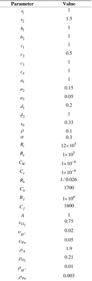
Here, a1, a2, and a3 are the different killing ef-fects of chemotherapy on the cell populations. Chemo-therapy drug decay rate in the blood stream is denoted by d2. The system parameters which are normalized to the maximum carrying capacity of the normal cells are given in Table 1. Analysis of the model for possible equilibrium points in the absence of therapy is given in the next sub-section.
In order now to generalize the dynamics of the cell in terms of electromagnetic model, heat transfer model, fluid transfer model, fractional mass model, cellular growth, let us introduce the state space dynamic vari- ables as follows.
Define the electric charge passing from or into the call ( )
V t as x5. Since the electric current flow is the rate of change of charge passing through an inductor I q
then
5 6 ( )
x x V t (27)
6 ( )
x V t (28)
Then the equivalent electric circuit Eq.4 can be re- expressed as
6( ) 2 6( ) 2 ( )5
( ) 2 ( ) ( )
i e w i w e w e e
i w ex ex e
R R C x t R C R C R C x t x t
R C V t V t u t
(29) The electric dynamics (29) can be modified as
6 6
5
2
2
( )
i w e w e e
i e w
e i e w
R C R C R C
x x
R R C
x u t
R R C
(30)
Furthermore, representing the heat model (9) in the state space form assuming x7 yields
7 7
1
h in out h h
x x R q
R C
Table 1. Overall dynamics parameters.
Parameter Value
1 r 1 2 r 1.5 1 b 1 2 b 1 1 c 1 2 c 0.5 3 c 1 4 c 1 1 a 1 2 a 0.15 3 a 0.05 1 d 0.2 2 d 1 0 s 0.33 0.1 0.3 i
R 12 10 5
e
R 5
1 10
W
C 6
1 10
e
C 1 10 6
h
R 1/ 0.026
h
C 1700
f
R 6
1 10
f C 1600 A 1 2 O 0.75 H
0.02
Pn 0.05 A 1.9 2 O 0.21 H
0.01
Pn
0.003
Similarly, for the cellular fluid transfer (13) assuming
8
x h will lead to
8 8
1
in f f
x x Q
R C
(32)
For the significant of the oxygen, pH and Pancreatin enzyme for the survival of the normal cell, their frac-tional mass ratio will be considered. Denote their corre-sponding masses, respectively, as
9 oxygene
x m , x10mH and x11mPancreatin (33)
Referring to (18) and (19), last Eq.33 can be reformu-lated as
i
i
i i i i v A i i
i
v A
m m m v Ah m v Ah
v A
(34)
By the virtue of the fluid dynamics equation the for-mer equation the fractional mass of the oxygen, pH and Pancreatin enzyme can be described, respectively, by
2
2 2
9 8 9
O
O A O in
f f v A
x x x v AQ
R C
(35)
10 8 10
H
A in
H H
f f
v A
x x x v AQ
R C
(36)
11 8 11
Pn
Pn A Pn in
f f
v A
x x x v AQ
R C
(37)
where
2 O
v ,
H
v and vPn are the fractional ratios of
oxygen, hydrogen as a measure of PH and Pancreatin, respectively. Fractional rate of change of the three sub-stances with respect to their initial values are defined,
respectively, as 2
2 2 O O O v v
, H H H v v
and Pn pn
Pn
v
v
along with the rate of change of the cell surface area
with respect to its initial value as A A
A . Selection of such substances are based on their significant role in the survival of human cell and killing or at least slowing down the tumor cells.
Now the overall generalized model is
1 1 1(1 1 1) 1 1 2 1 1 4
x r x b x c x x a x x (38)
2 2 2(1 2 2) 2 1 2 3 2 3 2 2 4
x r x b x c x x c x x a x x (39)
2 3
3 0 4 2 3 1 3 2 3 4
2
x x
x s c x x d x a x x
x
(40)
4 2 4 ( )
x d x u t (41)
5 6
x x (42)
6 6 5 2 2 ( )i w e w e e
i e w
e i e w
R C R C R C
x x
R R C
x u t
R R C
(43) 7 7 1
h in out h h
x x R q
R C
(44)
8 8
1
in f f
x x Q
R C
(45)
2
2 2
9 8 9
O
O A O in
f f v A
x x x v AQ
R C
10 8 , 10
H
A in
v H H
f f
v A
x x x v AQ
R C
(47)
11 8 , 11
Pn
v Pn A Pn in
f f
v A
x x x v AQ
R C
(48)
The overall generalized dynamics represents the bio- thermal electro-fluidic dynamics with 11 dimension. Next section will investigate the stability of the entire dynamical system at equilibrium points.
5.1. Equilibrium State
It is necessary to investigate the equilibrium state of the cell since it indicates its stability and the non-growth of the tumor cells. As a start, let us assume a free therapy and find out the corresponding equilibrium points for the dynamics (38)-(41).
As for the normal cells, equilibrium is governed by
1 1 1(1 1 1) 1 1 2 0
x r x b x c x x indicates that
1 0, 2 1(1 1 1) / 1, and when 2 1 1/ 1
x x r b x c x x b
Tumor cells equilibrium exists when
2 2 2(1 2 2) 2 1 2 3 2 3 0
x r x b x c x x c x x (49)
at points satisfy
2 0 and 2 (1/ 2) ( 2/ 2 2) 1 ( 3/ 2 2) 3
x x b c r b x c r b x
(50)
On the other hand, the immune system will experience equilibrium when
2 3
3 0 4 2 3 1 3
2
0
x x
x s c x x d x
x
(51)
at state
0 2
3
1 2 4 2 2 2
( )
( ) ( )
s x
x
d x c x x x
(52)
Provided that d1(x2)c x4 2(x2)x2
Finally with free therapy x40 at x40 with zero control input u t( ).
It can be seen easily that the system has three different types of equilibria: Tumor-free (no tumor cells), Dead
(no normal tissue cells), and Coexisting (both normal and tumor cells exist) equilibrium points [4]. In the con-text of developing therapy strategy, Tumor-free or Coex-isting type equilibrium points should be reached, since in these types of states, the normal cell population is close to its healthy state. In this study, our aim is to determine the therapy dosage to bring the system to the tumor-free
equilibrium point. The tumor-free equilibrium point of the system is obtained as (1/b2, 0,s0/d1, 0) which
gives us a healthy normal cell population of (1/b2)and
immune cell population of (s0/d1)with zero tumor
level and free drug injection. Considering now the
elec-tromagnetic equilibrium given that x5x60, along with
6 6 5
2 2
( ) 0
i w e w e e
e
i e w i e w
R C R C R C
x x x u t
R R C R R C
(53) when states x6x5u te( )0 which is not feasible since the live cell should keep a cellular voltage in the range of 80 - 100 millivolts. With other equilibrium state
6 5
2
( )
2 2
i e w
i w e w e e i w e w e e
R R C
x x u t
R C R C R C R C R C R C
(54) The human cell will have a steady-state heat transfer when
7 7
1
0
h in out h h
x x R q
R C
(55)
at
2
7 h h in h h out
x R C q R C (56)
A steady-state cellular fluid flow occurs when
8 8
1
0
in f f
x x Q
R C
(57)
8 f f in
x R C Q . (58)
Thus, the fluid steady-state occurs when
8 f f in
x R C Q . Fractional mass balance exist in the hu-man cell when the oxygen flow, PH and Pancreatin sat-isfy, respectively,
2
2 2
9 8 9 0
O
O A O in
f f v A
x x x v AQ
R C
(59)
10 8 , 10 0
H
A in
v H H
f f
v A
x x x v AQ
R C
(60)
11 8 , 11 0
Pn
v Pn A Pn in
f f
v A
x x x v AQ
R C
(61)
with oxygen equilibrium state given by
2
2
2 2
9 8
O O
in
f f O A O A
v A v
x x AQ
R C
(62)
and PH equilibrium state defined by
10 8
, ,
H H
in
f f v H A v H A
v A v
x x AQ
R C
(63)
Finally Pancreatin stability when
11 8
, ,
Pn Pn
in
f f v Pn A v Pn A
v A v
x x AQ
R C
equlibruim points for the purposed of control design.
5.2. Authors and Affiliations
It is desired at the moment to seek a linearized model of the cells growth at the equilibrium points with zero con-trol input in the given form
x Ax (64) where Ais the Jacobian Matrix. To fulfill this goal, let
1 1( ,1 2, 3, 4)
x f x x x x (65)
2 1( ,1 2, 3, 4)
x f x x x x (66)
3 1( ,1 2, 3, 4)
x f x x x x (67)
4 1( ,1 2, 3, 4)
x f x x x x (68)
The Jacobian matrix for the dynamics (38)-(41) can be verified as
1 1 1 1 1 2 1 1 1 1
2 2 2 2 2 2 2 1 3 3 2 4 3 2 2 2
3 2 2 3 2
4 2 2 4 1 3 3
2 2 2 1 2 0 2 ( ) 0 ( )
0 0 0
r r b x c x c x a x
c x r r b x c x c x a x c x a x
A x x x x x
c x a x d a x
x x d (69)
Substituting now the equilibrium point (1/b2, 0,s0/d1, 0) yields to the following linearized Jacobia Matrix
1 1 1 2 1 2 1 2
2 2 2 3 0 1
0
1 3 0 1
1
1
2 / / 0 /
0 / / 0 0
0 /
0 0 0
r r b b c b a b
r c b c s d
A s
d a s d
d d (70)
The following tables show the generalized system pa-rameters values used in the modeling and linearized state-feedback control.
This linearized overall dynamical model will be the interest of next section to investigate controllability, ob-servability and designing a state-feedback controller using pole placement approach. Later analysis will show
these parameters are so important in determining the stability of the human cell, its survival and in the growth of the tumor cells and decreasing the immune system. Some parameters affect the normal cells growth, tumor growth and immune system strength, cellular voltage, heat and fluid flow, oxygen rate, acidity and pancreatin enzyme.
2 2
1 1 1 2 1 2 1 2
2 2 2 3 0 1 0
1 3 0 1 1
1
2 / / 0 / 0 0 0 0 0 0 0
0 / / 0 0 0 0 0 0 0 0 0
0 / 0 0 0 0 0 0 0
0 0 0 0 0 0 0 0 0 0
0 0 0 0 0 1 0 0 0 0 0
2 2
0 0 0 0 0 0 0 0 0
1
0 0 0 0 0 0 0 0 0 0
1
0 0 0 0 0 0 0 0 0 0
0 0 0 0 0 0 0
i w e w e e
i e w i e w
h h
f f O
O f f
r r b b c b a b
r c b c s d
s
d a s d
d
d
R C R C R C
R R C R R C
A R C
R C v A R C
, , 0 00 0 0 0 0 0 0 0 0
0 0 0 0 0 0 0 0 0
A H A v H f f Pn
v Pn A f f v A R C v A R C (71) The input vector is given by
2
1 1 1 ( ) 1 ( )
T
e h in out in O in H in Pn in
6. CONTROLABILITY AND OF TUMOR
DYNAMICS AND CONTROLLER
DESIGN
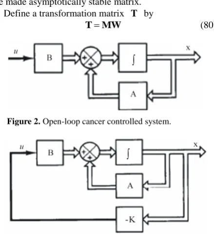
A system is said to be controllable at time t0 if it is possible by means of unconstrained control vector to transfer the system from an initial state x t( )0 to any other state in a finite interval time. The concepts of con-trollability and observability were introduced by Kalman. They play an important role in the design of control sys-tems in state space. In fact, the conditions of controlla-bility and observacontrolla-bility may govern the existence of a complete solution to the control system design. Although most physical systems are controllable and observable, corresponding mathematical models may not possess the property of controllability and observability. In what follows, we shall derive the condition for complete state controllability. Figures 2 and 3 show the open-loop cancer controlled systems and closed-loop cancer con-trolled system, respectively.
Consider the continuous-time system
w
x Ax B (73)
w
y Cx D (74) where,
x is a state vector
y is m-output vector
w is a control signal
A is n n matrix
B is n1 matrix
C is n m matrix
The system described in Eq.73 is said to be state con-trollable at tt0 if it is possible to construct an uncon-strained control signal that will transfer an initial state to any final state in a finite time interval t0 t t1. If every state is controllable, then the system is said to be completely state controllable [12]. The system is said to be controllable if and only if the following n n matrix is full rank n
B AB A B2 An 1B (75) This matrix is called the controllability matrix. A system is said to be observable at time t0, if with the system in state x t( )0 , it is possible to determine its state from the observation of the output over a finite time interval.
The concept of observability is very important be-cause , in practice, the difficulty is encountered with state feedback control is that some of the state variables are not accessible for direct measurement , with the re-sult that it becomes necessary to estimate the unmeasur-able state variunmeasur-ables in order to construct the control
signals. The system is said to be observable if and only if the following n nm matrix is of full rank n
T T T T T T T
2 n 1
C A C A C A C (76)
Matrix (76) is commonly called observability matrix. This following analysis presents a design method commonly called the pole-placement technique. We as-sume that all state variables are measureable and are available for feedback. It is shown that if the system considered is completely state controllable, then poles of the closed-loop system may be placed at any desired locations by means of state feedback through an appro-priate state feedback gain matrix. Let us assume the de-sired closed-poles are to be at s11, s22,…,
n n
s .
We shall choose the control signal to be
w Kx (77) This means that the control signal is determined by an instantaneous state. Such a scheme is called state feed-back. The 1n matrix K is called the state feedback gain matrix. Substituting (77) into Eq.73 gives
( )t ( )t
x A BK x (78)
The solution of this equation is give by
( )t (0)eA BK t
x x (79)
where is the initial state caused by external disturbances. The stability and transient response characteristics are determined by the egienvalues of matrix A BK . If matrix K is chosen properly, the matrix A BK can be made asymptotically stable matrix.
Define a transformation matrix T by
[image:10.595.316.536.462.706.2]T MW (80)
[image:10.595.324.527.606.702.2]Figure 2. Open-loop cancer controlled system.
Figure 3. Closed-loop cancer controlled system.
where M is the controllability matrix
B AB A B2 An 1B (81) and
1 2
2 3
1
1
1 0
1 0 0
1 0 0 0
n n
n n
a a a
a a
a
W (82)
where the a si are the coefficients of the characteristic polynomial
1
1 1
n n
n n
sIA s a s asa (83) Let us choose a set desired egienvalues as s11,
2 2
s ,···,snn. Then the desired characteristic equation becomes
1
1 2 1 1
(s )(s ) (s n) sn sn n s n
(84)
The sufficient condition that the system to be com-pletely controllable with all egienvalues arbitrarily placed by choosing the gain matrix
11 1 2 2 1 1
n an n an a a
K T
(85)
The former outlined control design will be validated in the following section by demonstrating the simulation results.
Simulation Results
Every cell in the human body functions as a micro bat-tery. To successfully bring nourishment in and take poi-sons out, it has to be fully charged. In a cancerous cell, the cell voltage drops from 90 millivolts to less than 40 millivolts. When the cell voltage gets to the very bottom, only 5 substances can pass in or out of the cell. They are water, sugar, potassium, cesium and rubidium [12]. Ox-ygen cannot enter into a cancer cell. Even if there is a lot of oxygen in the blood, it cannot get into the cell. Ce-sium, because of its electrical properties can still enter the cancerous cell. When it does so, because of its ex-treme alkalinity, the cell dies. Luckily, healthy cells are not affected by cesium because their cell voltage allows them to balance themselves. This uptake can be en-hanced by Vitamins A and C as well as salts of zinc and selenium. The quantity of cesium taken up was sufficient to raise the cell to the 8 pH range. Where cell mitosis ceases and the life of the cell is short.
The objective of the Cesium therapy is to kill the tu-mor cells, minimize the amount of drug application and to keep cellular voltage, thermo-fluid transfer and
cellu-lar ingredients at fixed rates. In the simulated general-ized cancer model, the healthy equilibrium point with the parameter set given in Table 1 is (1, 0, 1.65, 0, 0.1, 0, 7.4488 × 10⁶, 1.6 × 10⁶, 0, 0, 0) is locally stable. It means that the growth of cancer is controllable if suffi-cient drug surveillance is guaranteed.
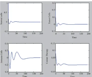
In the absence of sufficient immunee control, the tu-mor cells grow in number and kill the healthy tissue cells and reach the limit capacity, which is referred to as dead equilibrium point. The initial states, i.e., the conditions when the chemotherapy treatment is started, are assumed to be: N(0) = 1, T(0) = 0.20, I(0) = 1, M(0) = 1). The response of treatment-free cancer growth with respect to normalized time scale is given in Figures 4-6. Simula-tion analysis shows the following sensitivity of parame-ters that affect the cell stability.
The egienvalues of matrix A have some positive val-ues, zero, and imaginary with negative real values. Thus the original system is unstable. These egienvalues are listed as follows:
–0.0002 + 0.1291i, –0.0002 – 0.1291i –1.0000, –0.2000 –0.6500 –0.2000
–0.0000 2.0050 2.2100 2.0100 –0.0000
Since the original dynamics is unstable, it is now de-sired to design a state-feedback controller with the fol-lowing desired egienvalues: –0.1, –0.1, –0.2, –0.2, –0.3, –0.3, –0.4, –0.4, –0.5, –0.1, –0.1. As it can be seen, all desired eigenvalues are negative and close to the origin to guarantee a stable and fast response.
[image:11.595.52.284.81.236.2]Before proceeding in the controller design, the con-trollability condition defined by Eq.75 must be satisfied. Considering coefficient matrix A defined (71), the input vector given by (72), and parameters values listed in
Table 1, it is found out that the controllability matrix is of full rank 11.
Figure 4. Normal cells, tumor cells, immune cells and therapy input response.
[image:12.595.116.481.415.702.2]Figure 6. Fractional mass of oxygen, hydrogen ion and Pancreatin Enzyme.
by enforcing free kill cells.
Similarly, the cellular voltage is regulated at the re-quired value. Transfer of heat and fluid from and into the cell is maintained fixed as well. Since oxygen is so sig-nificant to maintain a healthy cell and reduce or kill the tumor cells its control was so efficient to keep the normal and immune cells as desired. Acidity is controlled by the amount of hydrogen ions in the cell as well. Finally, Pan-creatin ratio (which has an important role in killing tumor cells) is kept within the normal range as well.
If Ri109 or
9 10
e
R (Independently), the
system is unstable.
If both RiRe 107, the system is unstable.
IncreasingRi, immunity increases.
Decreasing Re, immunity increases significantly (20 times manifold).
Decreasing wall capacitance CW increases the nor- mal cells, tumor cells and immune cells and all oth-ers.
Increasing of area ratio A to 2.8, oscillations oc-curs; and at 2.9 it results in unstable cells.
Increasing oxygen ratio
2 O
to 3 will generate oscil-lations; and to 3.8 produces unstable cells.
Decreasing hydrogen ratio
H
to 0.01 and oxygen
rate
2 O
at 0.021 , generates unstable cells.
Increasing Pancreatin ratio Pn to 6 produces unsta-ble cells.
7. CONCLUSIONS
REFERENCES
[1] Hanahan, D. and Weinberg, R.A. (2000) The hallmarks of cancer. Cell Journal, 100, 57-70.
doi:10.1016/S0092-8674(00)81683-9
[2] Raines, J.K. (1981) Electromagnetic field interactions with the human body: Observed effects and theories. Technical Report, NASA, Goddard Space Flight Center, Washington.
[3] De Pillis, L.G. and Radunskaya, A.E. (2003.) The dy-namics of an optimally controlled tumor model: A case study. Mathematical and Computer Modeling, 37, 1221- 1244. doi:10.1016/S0895-7177(03)00133-X
[4] Itik M., Salamci, M.U. and Banks, S.P. (2010) SDRE optimal control of drug administration in cancer treat-ment. Turkish Journal of Electrical Engineering and Com- puter Sciences, 18, 715-729.
[5] Szymanska, Z. (2003) Analysis of immunotherapy
mod-els in the context of cancer dynamics. International Journal of Applied Mathematics and Computer Science, 13, 407-418,
[6] Byrne, H.M., Alarcon, T., Owen, R., Webb, S. D. and Maiki, P.K. (2006) Modelling aspects of cancer dynam-ics: A review. Philosophical Transaction of the Royal Society A, 364, 1563-1578.
[7] Kirschner, D. (2009) On the global dynamics of a model for tumor immunotherapy. Mathematical Biosciences and Engineering, 6, 573-583.
[8] U. Ledzewicz, (2005) Optimal control for a system mod-elling tumor anti-angiogenesis. ACSE 2005 Conference, Cairo, 19-21 December 2005.
[9] Ghaffari, A. and Nasserifar, N. (2009) Mathematical modeling and lyapunov-based drug administration in cancer chemotherapy. Journal of Electrical & Electronic Engineering, 5, 151-158.
[10] Warburg, O.H. (1969) The prime cause and prevention of cancer. 2nd Edition, Konrad Triltsch, Würzburg. [11] Brewer A.K. (1984) The high ph therapy for cancer, tests
on mice and humans. Pharmacology Biochemistry & Behavior, 21, 1-5.