ISSN Online: 2162-2086 ISSN Print: 2162-2078
DOI: 10.4236/tel.2018.811162 Aug. 22, 2018 2520 Theoretical Economics Letters
The Hedging Effectiveness of Malaysian Crude
Palm Oil Futures: An Application of the
Extended Mean-Gini Model
Kin-Boon Tang
*, Ju-Yau Tarn
Nottingham University Business School, The University of Nottingham, Malaysia Campus, Selangor, Malaysia
Abstract
This paper aims to demonstrate the superiority of Extended Mean-Gini (EMG) framework which is consistent with the second-order of stochastic dominance theory. The study provides a comprehensive analysis of investors’ distinct risk averse behavior towards optimal futures hedging strategy. The empirical distribution function method and the more efficient kernel estima-tion method are employed in the estimaestima-tion of EMG hedge ratios. Further-more, the moving data window procedure is used to examine the stability of the dynamic hedge ratios. The research is conducted on Malaysian Crude Palm Oil and CPO Futures markets for the period of 16th March 1995 to 28th June 2011. The empirical results show that the EMG approach is apparently more appropriate than the MV approach where EMG framework incorpo-rates the risk aversion factor. The study also shows the instability of dynamic hedge ratios across time horizons hence not favorable to investors who adopt the “buy and hold” strategy.
Keywords
Hedging Effectiveness, Crude Palm Oil Futures, Mean-Gini Approach, Financial Risk Management
1. Introduction
The Mean-Variance (MV) framework which is consistent with the normality (Gaussian) assumption is widely used by practitioners in futures hedging. It has been long noted by the quantitative finance community that most of the finan-cial asset returns are non-normal. The finanfinan-cial turmoil of 2008 is among many such rare and unpredictable financial crises over past decades that raise public
How to cite this paper: Tang, K.-B. and Tarn, J.-Y. (2018) The Hedging Effective-ness of Malaysian Crude Palm Oil Futures: An Application of the Extended Mean-Gini Model. Theoretical Economics Letters, 8, 2520-2549.
https://doi.org/10.4236/tel.2018.811162
Received: July 10, 2018 Accepted: August 19, 2018 Published: August 22, 2018
Copyright © 2018 by authors and Scientific Research Publishing Inc. This work is licensed under the Creative Commons Attribution International License (CC BY 4.0).
http://creativecommons.org/licenses/by/4.0/
DOI: 10.4236/tel.2018.811162 2521 Theoretical Economics Letters concerns in challenging the conventional ideas of portfolio optimization. Does the normality assumption hold for financial asset returns? If not, any alternative framework could potentially model the non-normally distributed asset returns? To address the problem, this study presents a stochastic dominance approach, the Extended Mean-Gini (EMG) framework, to measure the risk and hedging effectiveness in futures hedging strategies without restricted to the normality assumption.
As featured in past literatures and statistical phenomena, extreme events par-ticularly with negative returns appear to be more pronounced than predicted by a normal distribution [1] [2] [3]. Implications inherent in assuming normally distributed asset returns have become a famous area of interest for both inves-tors and researchers ever since. The normality assumption is essential in the sense that it could lead to econometrics biases and invalidates the evaluation of risk. Consequently, the conventional optimization model could significantly understate downside risk [4] [5] [6], thereby rendering an investor’s portfolio non-optimal.
Notwithstanding the renowned simplicity of MV framework and growing body of evidence suggest the assumptions of this framework are too restrictive. Stochastic dominance approaches are often proposed as the remedies for the de-ficiencies of the conventional MV approach. EMG framework proposes the use of Gini’s mean difference as an alternative measure of risk, thus possesses the theoretical dominance to model non-normal returns explicitly. It is an extension of the Mean-Gini (MG) model developed by Yitzhaki [7] to parameterize risk.
This study demonstrates the econometric advantages of using EMG frame-work in Malaysia’s Crude Palm Oil Futures (FCPO) market for futures hedging purposes. It deals with unconditional normality in which the returns distribu-tion of financial asset does not change through time. The study further focuses and illustrates the introduction of risk aversion into futures hedging strategy where investors’ risk appetite and tolerance level are incorporated in futures hedging.
There are immense amounts of studies regarding the hedging effectiveness and MV framework. One can easily find vast amount of literature of MV futures hedging that has been conducted on the financial markets. The well established studies that employed MV approach are Ederington [8], Figlewski [9], Herbst et al. [10], Lien and Luo [11], and Baillie and Myers [12]. These studies emphasized the use of different econometric models in modeling the spot and futures prices for developed and developing countries. Nevertheless, there are very limited re-sources on the EMG of the stochastic dominance approach in futures hedging. Some popular studies on the EMG proposed by Shalit and Yitzhaki [13] are Hodgson and Okunev [14], Kolb and Okunev [15], Lien and Luo [16] and Lien and Shaffer [17], among others. These studies focused mainly on equity indices and currencies hedging in developed countries. In contrast, very little empirical works in this area are for agricultural commodities under the EMG framework.
DOI:10.4236/tel.2018.811162 2522 Theoretical Economics Letters Stock Exchanges All Ordinaries Index (AOI) and found that EMG hedge ratios follow a step function of the underlying risk aversion parameter. However, con-trary to Hodgson and Okunev [14] and Kolb and Okunev [15], Lien and Luo
[16] shown that EMG hedge ratio is a smooth function of risk aversion parame-ter. Lien and Luo’s [16] research was based on the S & P 500 index using the kernel estimation method. While accessing the stability of the hedge ratios, Lien and Luo [16] demonstrated a step function of hedge ratio for high risk aversion parameter but not for low degree of risk aversion. That is, contrary to the find-ings of Hodgson and Okunev [14]. Such conflicting results indicate that there has yet been any concrete finding on the EMG hedge ratio function. Not to mention that most researches were based on indices and currencies hedging while very minimal are done on agricultural commodities.
Despite the fact that Malaysian FCPO is the most actively traded commodity futures in emerging markets of Asia, existing studies were relatively low com-pared to other developed futures market. Some of the financial researches re-garding FCPO futures market are returns and volatility [18], market efficiency
[19], spillover effect [20] and cointegration analysis between CPO and FCPO prices [21]. More recently, works done on FCPO futures hedging includes con-ventional MV hedging [22], dynamic hedging [23] and comparison between constant and dynamic hedge ratios [24]. These studies on futures hedging were constructed under the assumption of normality returns of assets. In fact, it is necessitate examining the risk aversion factor on hedging performance of FCPO under EMG framework which will not be invalidated by the non-normality of returns.
In conjunction with the few studies done on agricultural commodities futures, this study aims to examine the superiority of EMG approach over the MV framework in hedging crude palm oil prices. The study will investigate how the risk aversion factor would have affect the hedge ratio and hedging effectiveness and evaluate the EMG hedge ratios using two different estimation methods; the ranking and the kernel estimation method. The appropriateness of the “buy and hold” strategy in futures hedging strategies will then be examined at the end of the study.
ap-DOI: 10.4236/tel.2018.811162 2523 Theoretical Economics Letters proach. This study will complement those and adds to the existing literature of EMG futures hedging CPO studies. For this purpose, in Section 2, we will ex-plain the methodology and theoretical foundation of EMG approach in futures hedging. In Section 3, the empirical results are presented and discussed. The findings shed lights on how risk aversion factor would affects the optimal hedge ratios for different classes of investors. The last Section 4 concludes and provides recommendation to investors.
2. Model Specification
2.1. The OLS Model of MV Framework
The traditional approach [8] [9] uses univariate OLS regression to find Mini-mum-Variance Hedge Ratio (MVHR) estimates. The OLS linear regression model is given by
, ,
s t f t t
R = +α βR +ε
where εt is the residual from OLS regression and β is the MVHR.
Edering-ton [8] defined hedging effectiveness as the reduction of hedged portfolio’s va-riance compared to unhedged portfolio. The returns for unhedged and hedged portfolio are simply expressed as
, u s t r =R
*
, ,
h s t f t
r R= −h R
respectively, where ru and rh are the return of unhedged and hedged
portfo-lios respectively while h* denotes the estimated MVHR. Hence, the hedging effectiveness [8] can be expressed as
( )
( )
( )
Var U Var H HEVar U − =
where Var U
( )
and Var H( )
are corresponding variances of unhedged port-folio and hedged portport-folio. That is, hedging effectiveness is a measure of the percentage of variance reduction when portfolio is hedged at MVHR.2.2. Mean-Gini Framework
While the first assumption of mean-variance portfolio theory, the normally dis-tributed returns of financial asset is violated, the second assumption of quadratic utility implies an implausible conclusion of all investors exhibiting growing ab-solute risk aversion. In other words, the second assumption mentioned also im-plies all investors have homogeneous risk attitudes in investment decision mak-ing. The MG framework which consistent with the stochastic dominance rules and the principle of maximizing expected utility is not accountable to these criti-cisms of MV portfolio theory. The MG framework developed by Yitzhaki [7] [25]
DOI:10.4236/tel.2018.811162 2524 Theoretical Economics Letters The Gini’s mean difference is the measure of the variability of a risky prospect. This Gini coefficient was named after an Italian mathematician Corrado Gini in honour for his development of this risk measure. In an investment context, the Gini’s mean difference can be interpreted as magnitude variation between two asset returns randomly draw from a probability distribution. Suppose random draws are carried out repeatedly with a pair of returns at a time, the magnitude difference is observed for the whole process. A pair of returns drawn from a widely dispersed distribution will tend to have a large magnitude difference while the pair from a narrowly dispersed distribution tends to have a smaller magnitude difference.
The Gini coefficient captures the expected value of the magnitude difference by two statistics, the mean and the Gini’s measure of dispersion. The MG framework therefore provides a necessary condition for second order stochastic dominance despite the distribution of the financial asset return. Hence, poten-tially a better framework than the MV approach. Following the approach of Yitzhaki [25] and let R1 and R2 denote the random returns drawn from the same probability distribution, the Gini coefficient Γ is defined as
1 2
1
2E R R
Γ = −
Assume the random return R is bounded by [a, b] such that F (a)= 0 and F (b) = 1. In practice, this algebraic expression can be expressed in a more convenient form as below
( )
( )
21 d 1 d
b b
a F r r a F r r
Γ =
∫
− −∫
− Alternatively, the Gini coefficient Γ is analytically equivalent to
( )
{
}
2cov , 1r F r
Γ = − −
The Gini coefficient expressed in covariance form of two random variables is more easy and convenient for computations in empirical studies. This MG mod-el is a special case of the Extended Mean-Gini modmod-el with a degree of risk aver-sion of 2, which will be discussed in the next section.
2.3. The Extended Mean-Gini (EMG) Framework
Yitzhaki [7] and Shalit and Yitzhaki [13] enhanced the Gini coefficient by ex-panding it into a family of coefficients of dispersion. Each coefficient of the Ex-tended Gini family is defined by parametrising the risk attitudes of practitioners with parameter v. The EMG coefficient Γ
( )
v can be expressed as( )
v ab 1 F r( )
dr ab 1 F r( )
vdrΓ =
∫
− −∫
− where 1≤ < ∞v .The parameter v which represents the risk aversion levels is a
DOI: 10.4236/tel.2018.811162 2525 Theoretical Economics Letters lower portion of the cumulative distribution, reflecting a higher concern for the downside risk. This also implies they are eager to pay higher premium to miti-gate the risk taken.
Yitzhaki [7] classified risk seekers as having a value between 0 and 1 for the risk aversion parameter, which is 0≤ <v 1. When of v=1, it represents inves-tors with risk neutral behaviour as Γ
( )
1 0= . An investor with risk-neutralbe-havior would have no preference over available investment options, therefore having an EMG coefficient of zero. On the other hand, risk averse investors are identified by parameter v≥2. A more risk averse practitioner will adopt a
greater parameter v while v as tends to infinity, the person is implementing a strategy which minimising the possible loss for a worst scenario. The EMG coef-ficient Γ
( )
v was proved [13] to take a much simpler covariance form as follow( )
{
( )
1}
cov , 1 v
v v r F r −
Γ = − −
where cov .,.
( )
denotes the covariance operator. It should be noticed that the Gini coefficient is a member of EMG family, a special case where v=2 thusgiving Γ = Γ
( )
2 . It has been shown that the Γ( )
v is bounded from above and a non-decreasing function of v. The approach which uses the EMG coefficients to formulate a hedging strategy is called the EMG approach.2.4. The EMG Approach in Futures Hedging
Yitzhaki [25] has derived the MG model in comparing uncertain prospects in portfolio analysis. Suppose two portfolios X and Y and let F
( )
. and G( )
. denote the cumulative distribution of these portfolios’ returns respectively. Ac-cording to Yitzhaki [25], the following inequality is necessary for prospect X to dominate prospect Y by first and second order of stochastic dominance efficien-cy( )
( )
1 d 1 d , 1,2,3,
b b
a a
v v
F r r G r r v
− ≥ − =
∫
∫
By letting v=1, it reduces to
X Y
µ ≥µ
where µX and µY are the expected return of prospects X and Y respectively.
The above result can then be generalized for the Extended Gini coefficient. Ac-cording to Shalit and Yitzhaki [13]:
( )
21 d
b a
a F r r
µ
Γ = − −
∫
− For the case of v=2,
( )
2( )
21 d 1 d
b b
a −F r r≥ a −G r r
∫
∫
( )
2( )
2X X Y Y
µ
− Γ ≥µ
− ΓDOI:10.4236/tel.2018.811162 2526 Theoretical Economics Letters
X Y
µ ≥µ
and
( )
( )
X X v Y Y v
µ
− Γ ≥µ
− ΓIf prospect X satisfied the two conditions above, then it is said to be EMG effi-cient and contained within the stochastic dominance effieffi-cient set, which is not subject to the faults usually advanced from the MV efficient set. Prospect X will remains within the EMG efficient set before a new portfolio comes across to stochastically dominate prospect X.
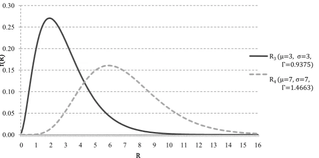
The stochastic dominance decision rules of EMG method can be demonstrat-ed by the following two simple examples each with different expectdemonstrat-ed return prospects. First, consider two uniformly distributed prospects with no overlap-ping distribution where R1 between 0 and 1 while R2 between 2 and 4. Clearly, investors will choose R2 due to its higher expected return but the MV approach rules out R2instead of R1 because of the greater variability of R2. Following sto-chastic dominance rules, the cumulative distribution of R2 always lay on the right of the cumulative distribution of R1 (
µ
R2>µ
R1), therefore R2dominate R1stochastically and lies within the EMG efficient set. Next, consider two Gamma distributed prospects R3 (mean = 3, variance = 3, Γ = 0.9375) and R4 (mean = 7, variance = 7, Γ = 1.4663) as depicted in Figure 1. In this case, investors would prefer R4but MV approach will opt for R3. Since
µ
R4− Γ >R4µ
R3− ΓR3, the EMGrules will discard R3 and remains R4in the EMG efficient set, thus forces the in-vestor to consider R4 only.
The empirical applications in this study focus on using Γ
( )
v as an index of different classes of investors, reflecting their risk aversion levels. Analogous to the MV framework by minimizing the variance, this approach minimize Γ( )
vconditional on v to obtain an optimal hedging strategy.
2.5. The Empirical Application of the EMG Approach
[image:7.595.216.535.542.700.2]Follows the approach adopted by Cheung et al. [26] and Hodgson and Okunev
Figure 1. The Evaluation of Two Gamma Distributed Prospects.
0.00 0.05 0.10 0.15 0.20 0.25 0.30
0 1 2 3 4 5 6 7 8 9 10 11 12 13 14 15 16
f(
R) R3 (µ=3, σ=3,
Γ=0.9375)
R4 (µ=7, σ=7,
Γ=1.4663)
DOI: 10.4236/tel.2018.811162 2527 Theoretical Economics Letters [14], a portfolio with long position on underlying asset and short position on futures contracts is created. In this case, a hedged portfolio of buying crude palms oil and shorting the FCPO contracts in BMD Berhad. The hedged portfo-lio’s return, Rp,t is given by
, , ,
p t s t f f t R =R −X R
where Xf is the EMG hedge ratio. The empirical implementation of the EMG coefficient as suggested by Lerman and Yitzhaki [27] is eased by minimizing the covariance form of EMG coefficient
( )
{
( )
1}
cov p, 1 p v
v v R F R −
Γ = − −
For empirical computation, the above equation is estimated by the corres-ponding sample analog. Thus, it can be rewritten as
( )
(
( )
)
1 ,(
( )
)
1, , ,
1 1 1
ˆ ˆ
1 1
T v T T v
p t
p t p t p t
t t t
R v
S v R F R F R
T T
− −
= = =
Γ = − − − −
∑
∑
∑
The computation process of equations above will be further discussed in the next section. In accessing the performance of the hedging strategy, consideration will be given to the degree of risk reduction conditional to risk aversion levels. Analogous to the risk-return framework proposed by Ederington [8], hedging effectiveness is defined as the percentage of risk reduction achieved from the op-timum hedging strategy. Similarly, with EMG coefficients, the hedging effec-tiveness [10] [28] can be expressed as
( )
( )
1 p s R R v HE v Γ = − Γwhere ΓRp
( )
v and ΓRs( )
v are the EMG coefficients for hedged andun-hedged portfolios respectively. Since no position in futures is taken for unun-hedged portfolio, the Gini for unhedegd portfolio is equivalent to the Gini of spot port-folio.
2.6. Estimating the EMG Coefficients
As shown in previous section, the EMG coefficient is expressed in term of EMG hedge ratio. By expanding it, then partial differentiating it with respect to EMG hedge ratio in order to obtain the global minimum Gini coefficient, the optimal EMG hedge ratio can be expressed as
( )
{
}
( )
{
}
1 1cov , 1
cov , 1
v
f p
f v
f p
f
R F R
X
R F R
X − − − − = ∂ − ∂
DOI:10.4236/tel.2018.811162 2528 Theoretical Economics Letters However, the denominator is difficult to evaluate empirically. Due to the com-putational complexity of the first derivative of EMG coefficient, an iteration technique [14] [15] is used to obtain the optimal hedge ratio. This grid search procedure involves a process where the hedge ratio, Xf is arbitrarily fixed in advance. With predetermined Xf , the Rp t, and Γ
( )
v can be calculated us-ing S vΓ( )
for a user-determined parameter v. In order to find the global minimum of EMG coefficient, this searching procedure is frequently repeated with different Xf values. That is, to find the minimum EMG coefficient over the choices of hedge ratios. In spite of that, the true distribution of returns is, of course, unknown. The next section will introduce the estimation methods for cumulative distribution for asset returns, namely, the ranking method [27] and the kernel density estimation suggested by Lien and Luo [16].2.7. The Ranking Method
Conventionally, the cumulative density function (CDF) is estimated by the ranking method [27]. The estimated F R
( )
p t, , also known as the empirical dis-tribution function (EDF) approach which is accomplished by ranking Rp t, and divides it by the number of observations. First, rank the observed portfolio re-turns Rp in an ascending order yielding Rank( )
Rp t, . Then, the complement of the estimated CDF can be expressed as( )
(
)
( )
,,
ˆ
1 p t p t
N Rank R F R
N −
− =
Hence raised the complement of CDF to the power of v−1 gives
( )
(
)
1( )
, 1,
ˆ 1
v
v p t
p t
N Rank R F R
N
−
− −
− =
It should be noted that higher ranked returns will gives lower complement CDF, and raising them to the power of v−1 for v greater than two will drive these term towards zero. As v tends to infinity, this will converge to zero; an in-tuitively appealing idea of the EMG framework. This is based on the EMG framework that greater risk averse investors will emphasize on lower end of the distribution while truncating the upper end of the distribution, giving more at-tention to the tendency of worse outcome than the possibility of great portfolio’s return. However, the simplicity of this estimation method is based on the fol-lowing presumption [16]
( ) ( )
, ,ˆ p t ˆ p t ,
F R ≠F R ′ t t≠ ′
DOI: 10.4236/tel.2018.811162 2529 Theoretical Economics Letters an alternative CDF estimation method is needed.
2.8. The Nonparametric Kernel Density Estimation
Lien and Luo [16] introduced the nonparametric kernel density estimation into the EMG framework. A nonparametric approach is used instead of the ranking method in estimation the CDF. This kernel smoothing method is applied by Lien and Luo [16], Lien and Shaffer [17] and Shaffer [29]. It is a more powerful CDF estimation which is known to produce efficient results with a smaller sam-ple. Reiss [30] asserted that an appropriately chosen kernel estimator is more ef-ficient than the empirically derived estimates. The kernel density estimates,
( )
ˆ .
F , evaluated at Rpt is
( )
1
1
ˆ N pt pi , 1,2, ,
pt
i T
R R
F R K t N
N =
α
−
= =
∑
where
( )
d 1k x x ∞
−∞ =
∫
and
( )
x( )
dK x =
∫
−∞k x xThe function K x
( )
and parameter αT are selected by the user. K x( )
isthe kernel density function which is, in this study, adopted the Gaussian kernel. That is, the probability density function for K x
( )
is chosen to be the standard normal random variable( )
1 e 222π
x
k x = −
The smoothing bandwidth αT is the parameter that affects the smoothness
or roughness of the resulting density estimate. Since the resulting estimated CDF is insensitive to the kernel function used, the choice of kernel is generally less important. However, the selection of bandwidth parameter is essential in kernel density estimation. Over-smoothing will occur if αT is too large and the nature
of the distribution will be obscured. If αT is too small, the kernel estimation
method will draws too much inference from the sample and leads to the un-der-smoothing of the CDF estimates. A procedure of selecting the optimum bandwidth is suggested by Silverman [31]:
1 5
0.9 , where min ,
1.34
T AN A IQR
α = − = σ
The σ denote the standard deviation; IQR represents the inter-quartile range of the data; min .,.
( )
denotes the minimum function in statistics. Silver-man [31] found that the above smoothing bandwidth works very well with wide variety of densities and is an adequate choice of bandwidth for many purposes. This optimum smoothing bandwidth is applied by Shaffer and DeMaskey [32]DOI:10.4236/tel.2018.811162 2530 Theoretical Economics Letters
2.9. The Moving Data Window
The methodology discussed above is based on a buy and hold strategy where the optimal hedge ratios is estimated for the whole sample period of approximately 16 years. Now, consider how investors might want to correct their hedge ratios accordingly to newly available information every day. Following Hodgson and Okunev [14], Kolb and Okunev [15] and Lien and Luo [16], the moving data window procedure is used to examine the stability of EMG hedge ratios across time. This multi-period consideration appears appropriate because futures posi-tions are marked to the market daily where the profits and losses are accounted daily. The moving data window procedure continuously re-evaluates the optimal EMG hedge ratios for every trading day. Consequently, the portfolio’s return can be written as
, , , ,
p t s t f t f t R =R −X R
where Xf t, represents the dynamic EMG hedge ratios. As asserted by Lien and Luo [16], this approach is insensitive to the moving data window selection. In the study, these hedge ratios are estimated based on previous 500 trading days; a moving window of 500 trading days which consists of 500 data points. It is as-sumed that investors re-evaluate the optimal hedge ratios based on most recent five 500 days of trading activities, wherein the newest data point replaces the most obsolete data point as the data window moves. Hence, for an input of pa-rameter v, this procedure will gives 3422 hedge ratios which is represented by
, f t
X . Both ranking method and the kernel density estimation are used for esti-mating the CDF in moving data window.
3. Data and Empirical Results
3.1. Data
The study uses two data series of crude palm oil: 1) the Malaysia Crude Palm Oil (CPO) spot prices, and 2) CPO Futures (FCPO) prices. The daily data are ob-tained from Bloomberg over a period of approximately 16 years, from 16th March 1995 to 28th June 2011. There are 3922 observations in total. The Malay-sia’s FCPO is considered as the most actively traded commodity futures in emerging commodity market. The prices of the data series are the settlement price based on last minute trading of the trading days. Meanwhile, the futures price referred to is the daily settlement price of nearby contract, taken from the nearest contract expiration. It represents the price per ton for each of the 25 me-tric tons of the futures contract. The FCPO contracts of Bursa Malaysia Deriva-tive Berhad are traded daily excluding non-business day. The return of an asset for a particular period is calculated as the difference between the natural loga-rithm of the price at the end of the period and the natural logaloga-rithm of the price at the beginning of the period.
DOI: 10.4236/tel.2018.811162 2531 Theoretical Economics Letters empirical distribution function (EDF) estimation method and subsequently the kernel estimation method in estimating the EMG hedge ratios. The EMG hedge ratios estimated by both methods are then compared. Since the hedge ratio will significantly affect the hedging performance of hedged portfolio, the measures of hedging effectiveness are evaluated and analyzed in both EMG framework and MV framework. Next, the study will appraise the appropriateness and suitability of the “buy and hold” strategy in FCPO hedging. To do so, the moving data window procedure is employed to consider thoroughly the time-series characte-ristics of EMG dynamic hedge ratios for different level of risk aversion. The principal issue here is to access whether investors of distinct risk preferences who hedged with MV hedge ratios are in-optimal.
In order to examine the normality of both CPO returns series, goodness of fit tests are performed using Shapiro-Wilk and Jarque-Bera normality tests. These robustness tests investigate how well the mentioned data series can be fitted into normal distribution. The normality null hypotheses are rejected, implying both returns are non-normally distributed. Hence, the EMG framework is more ap-propriate than the MV framework for modeling the CPO and FCPO returns. However, it is notable to mention that the EMG framework works well with or without the normality assumption of the returns series. Consequently, the EMG method is valid regardless of the results of these tests and is econometrically better than MV approach.
Breusch-Godfrey and Ljung-Box Q’ tests are applied to test the presence of autocorrelation. Autocorrelation up to order five is tested and shown that auto-correlation exists in the OLS model. Thus, the MVHRs produced by OLS model are biased estimates. Furthermore, White’s test and Breusch-Pagan test are em-ployed to detect the occurrence of heteroscedasticity of the return series. Based on the OLS regression model the null hypothesis of homoscedasticity is rejected for both tests. The results of the tests can be obtained upon request from the corresponding author.
3.2. The MV and MG Hedge Ratios
The most direct and less complex technique of computing the MVHR under MV framework is the conventional Ordinary Least Square (OLS) regression. First, an OLS regression of CPO returns on FCPO returns is executed to obtain the MVHR. The OLS regression results and other relevant information are summa-rized in Table 1.
The constant intercept 𝛼𝛼 is shown to be statistical insignificant which indi-cates the absence of the magnitude difference between the two return series. Contrary, the coefficient of the independent variable Rf is statistical significant at 5% level. The coefficient of Rf represents the MVHR of an optimal portfolio generated by the OLS model. The statistical results imply that investors should hedge the CPO’s price risk optimally at a hedge ratio of 57.62%.
DOI:10.4236/tel.2018.811162 2532 Theoretical Economics Letters Table 1. The OLS regression results.
Coefficient Std. error t-statistics Constant (α) 0.000041 0.000189 0.2179
f
R 0.576232 0.010729 53.71*
R-squared 0.423980
Note: a) The dependent variable is Rf; b) * denotes the test statistics is significant at 5% level; c) The
re-sults are based on the regression model Rs t, = +α βRf t, +εt. d) R-squared measures the hedging
effec-tiveness of MVHR; the percentage of risk reduction.
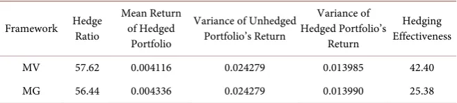
Hence, by adopting the MVHR of 57.62%, one can achieved a hedging perfor-mance of 42.40%. In short, the hedgers or investors could reduce the price risk by 42.40% as measured by the variation of portfolio’s return. As mentioned pre-viously, the non-normally distributed CPO and FCPO returns will invalidate the MV model. This is because the significance of t-statistics is mainly due to the non-normal distribution of returns rather than the causal relation between CPO spot and futures returns. Thus, the MG model is applied to counter with this econometric problem.
An MG regression based on the iterative grid searching procedure is per-formed to obtain the MG hedge ratio. The empirical results of MG model are reported in Table 2. This stochastic dominance model has predicted an optimal hedge ratio of 56.44%. It is noticed the Gini coefficient for a hedged portfolio is lower than the unhedged portfolio therefore implying lesser risk associated with the corresponding hedged portfolio. Indeed, the MG hedge ratio provides a no-ticeable risk reduction for the hedged portfolio over the sample period. A CPO spot position hedger would be able to achieve approximately 25% of risk reduc-tion. As a consequence, it signifies that FCPO contracts are still the potential hedging derivatives to hedge against CPO price risk even when the assumptions of normality returns are relaxed. Additionally, it is worthwhile to compare and scrutinize both MV and MG model side-by-side.
DOI: 10.4236/tel.2018.811162 2533 Theoretical Economics Letters Table 2. MG regression results.
Hedge Ratio Unhedged Portfolio Gini Coefficient on Gini Coefficient on Hedged Portfolio Effectiveness Hedging
56.44% 0.007893 0.005889 25.38%
[image:14.595.210.539.188.262.2]Note: (a) Hedging effectiveness measures the percentage risk reduction as computed by the Gini’s coeffi-cients.
Table 3. Comparisons between MV and MG framework.
Framework Hedge Ratio Mean Return of Hedged Portfolio
Variance of Unhedged Portfolio’s Return
Variance of Hedged Portfolio’s
Return
Hedging Effectiveness
MV 57.62 0.004116 0.024279 0.013985 42.40 MG 56.44 0.004336 0.024279 0.013990 25.38 Note: (a) The hedging effectiveness is computed by the corresponding risk measures of each framework re-spectively. Hence are not directly comparable.
3.3. The EDF Hedge Ratios
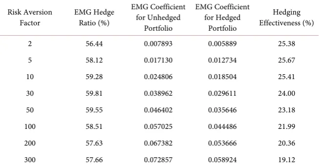
The iterative searching procedure prescribed in previous section is applied to various investor-specific risk aversion parameters (v); the EMG coefficient is minimized to obtain the EMG hedge ratios. In particular, the EMG coefficient is estimated for v values ranging from two to thirty incrementing by one, and from thirty-two to three hundred with increment of two. Also, the initial risk aversion factor (v = 2) is identical to the MG approach. In addition, risk aversion factor greater than three hundred are being considered in this study. However, these higher degrees of risk aversion factor for extremely risk averse hedgers did not produce hedge ratios significantly differ from those obtained in the above range. Therefore, these results are not reported here.
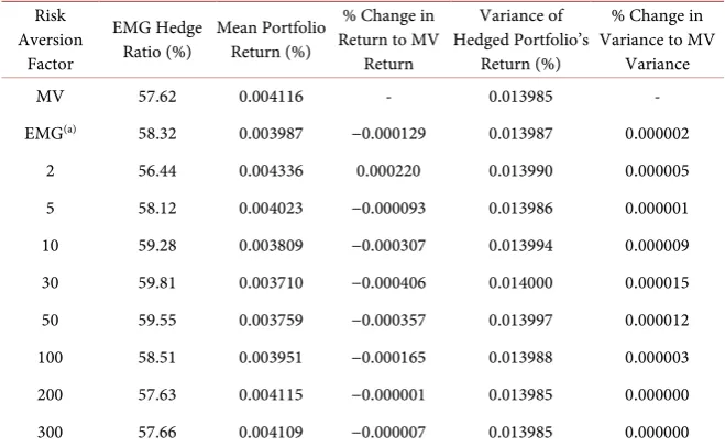
Table 4 briefly reports the results of estimated EMG for selected risk aversion parameter. It highlights a few important characteristics of EMG hedge ratios. First of all, it is empirically found that the EMG hedge ratios for Malaysian CPO markets do not follow a monotonic function. It is neither an increasing nor de-creasing pattern with regard to the risk aversion factor. This essential and mea-ningful characteristic will be discussed in detail later with a better comparative analysis with MVHR.
On the other hand, different degree of risk aversion investors has distinct EMG coefficients for the same unhedged portfolio, to be precise, the CPO spot position. Since risk averse hedgers would increasingly concerning the downside of CPO price risk, it is not surprising that they would perceived greater risk to the same CPO spot position. This distinctive characteristic of risk aversion is captured and reflected by the EMG’s measure of risk. The EMG coefficients for the unhedged portfolio are monotonically increasing with risk aversion factor. Therefore testifies the relationship between the investors’ risk behavior and per-ceived price risk exposure.
DOI:10.4236/tel.2018.811162 2534 Theoretical Economics Letters Table 4. EDF hedge ratios for various risk aversion parameters.
Risk Aversion
Factor EMG Hedge Ratio (%)
EMG Coefficient for Unhedged
Portfolio
EMG Coefficient for Hedged
Portfolio
Hedging Effectiveness (%)
2 56.44 0.007893 0.005889 25.38 5 58.12 0.017130 0.012734 25.67 10 59.28 0.024806 0.018504 25.41 30 59.81 0.038962 0.029611 24.00 50 59.55 0.046402 0.035646 23.18 100 58.51 0.057025 0.044486 21.99 200 57.63 0.067382 0.053666 20.36 300 57.66 0.072857 0.058924 19.12 Note: (a) A higher risk aversion factor indicates the investor is more concerns about the downside risk, hence more risk averse.
same spot position and thus raise the values of risk measure (EMG coefficients), indicating they are more concerning on the tendency of negative outcome on their spot position. Considering the impossible task to eliminate the possibility of negative returns and the incapability of futures contracts to ideally hedge all downside risk, it is reasonable that more conservative and risk averse investors will inflates their perceived risk exposure accordingly. If not, the mechanism of the market itself which would in turn otherwise created an arbitrage opportunity where hedgers will not suffer losses.
As they perceived much greater risk on the spot position, the same FCPO contracts who act as an effective hedging tool can therefore eliminate only a smaller portion of the risk perceived when the portfolio is optimally hedged. Thus, renders the deteriorating of hedging performance as risk aversion factor increases. In general, the FCPO contracts could provide approximately 20% or more risk reduction for CPO hedgers and investors.
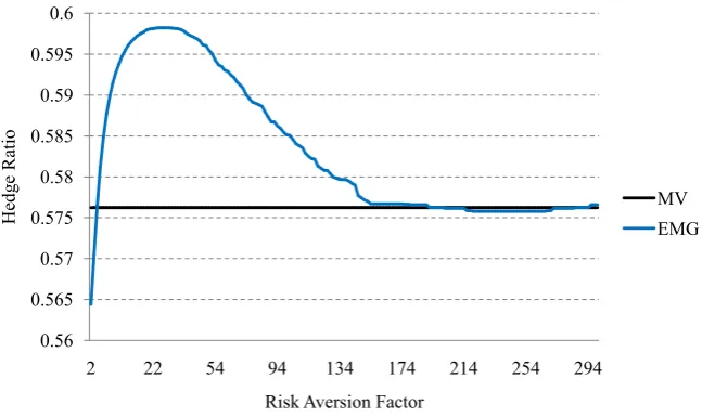
Figure 2 depicts the results of estimated EMG hedge ratios in comparison with the MVHR. Note that, the optimal hedge ratio varies across different degree of risk aversion. There are some important findings. First, the EMG hedge ratios are significantly different from the MVHR. Optimal hedge ratios for lower levels of risk aversion are generally different from the MVHR, for instance, hedge ra-tios for v = 5 to v = 100 are much greater than the MVHR. Meanwhile, the aver-age EMG hedge ratio (58.32%) is also higher than the MVHR. The MVHR is clearly inappropriate for less risk averse investors. Second, changes in hedge ra-tios can produce considerable deviations in portfolio returns but insignificant to variance of portfolio returns. In fact, shorting higher portion of FCPO contracts will produces lesser mean returns but would not significantly affects variance of returns. Third, less risk averse hedgers with similar risk aversion levels can have significantly differ optimal hedge ratios. For low levels of risk aversion (v = 5 to
DOI: 10.4236/tel.2018.811162 2535 Theoretical Economics Letters Figure 2. EMG Hedge Ratios (EDF Estimation Method) for FCPO.
Fourth, highly risk averse investors tend to have more stable and steady hedge ratios which are similar to the risk minimizing MVHR. The hedge ratios for v > 300 are almost constant (the results are not reported here). For extremely risk averse investors, it would be indifferent to adopt the MVHR or EMG hedge ratio as both framework give similar optimal hedge ratio. Consistent with the theoret-ical of EMG coefficient, as risk aversion increases, the EMG hedge ratio is being calculated with respect to an increasingly smaller subset of observations, hence severely constraining the potential changes of the hedge ratio. Fifth, the EMG hedge ratios show an asymmetric bell-like curve rather than a monotonic func-tion. This is a unique and appealing characteristic of FCPO market where the hedge ratio peaked at a risk aversion level v = 25.
Intuitively, one would expect that as investors are increasingly more risk averse, they would short more futures contract to diversify the risk. As investors become more risk averse, they are more pessimistic about their expectation and therefore seek to cover their position by shorting more FCPO contracts. This is, of course, due to their risk behavior of weighting negative outcome more than positive outcome. However, this explanation is partially true for the Malaysia’s CPO market. As less risk averse hedger become increasingly risk averse, the hedge ratio will be adjusted accordingly upward indicating the person will short more futures contracts to cover their position. Nevertheless, a reversal pattern is observed wherein the hedge ratio peaked at 59.82% (v = 25) then showing a downward trend signifying hedger should hedge with lesser FCPO contracts as the person is becoming more risk averse.
To analyze this results thoroughly, the returns on both CPO and FCPO are considered. Table 5 illustrates the returns of hedged and unhedged portfolios. For lower degree of risk aversion, as CPO investors are more risk averse, short-ing more FCPO contracts is presumably offset their CPO exposure with reduc-tion in risk while causing lower level of return simultaneously. It should note
0.56 0.565 0.57 0.575 0.58 0.585 0.59 0.595 0.6
2 22 54 94 134 174 214 254 294
H
ed
ge R
at
io
Risk Aversion Factor
DOI:10.4236/tel.2018.811162 2536 Theoretical Economics Letters Table 5. Comparison of EDF hedge ratio with MVHR.
Risk Aversion
Factor
EMG Hedge
Ratio (%) Mean Portfolio Return (%)
% Change in Return to MV
Return
Variance of Hedged Portfolio’s
Return (%)
% Change in Variance to MV
Variance MV 57.62 0.004116 - 0.013985 - EMG(a) 58.32 0.003987 −0.000129 0.013987 0.000002
2 56.44 0.004336 0.000220 0.013990 0.000005 5 58.12 0.004023 −0.000093 0.013986 0.000001 10 59.28 0.003809 −0.000307 0.013994 0.000009 30 59.81 0.003710 −0.000406 0.014000 0.000015 50 59.55 0.003759 −0.000357 0.013997 0.000012 100 58.51 0.003951 −0.000165 0.013988 0.000003 200 57.63 0.004115 −0.000001 0.013985 0.000000 300 57.66 0.004109 −0.000007 0.013985 0.000000 Note: (a) The EMG hedge ratio is calculated as the mean of all estimated EMG hedge ratios while other re-lated information are computed based on this average hedge ratio.
that both CPO and FCPO give an average of positive returns with FCPO records considerably higher return. While a FCPO hedging strategy involved shorting more FCPO contracts, the portfolio returns will be discounted by the losses rea-lized on the FCPO short position. Therefore, a sufficiently higher hedge ratio would produce an unfavorable negative mean returns where selling more FCPO contracts leads to lower returns.
On the contrary, in understanding the reversal pattern of a downward hedge ratio function, backwardation is hypothesized as the possible explanation [14]. Notice that, normal backwardation occurs more often, mostly than not, during the sample period. Hence, convenience yield arises whenever the CPO market is backwardated where CPO price is greater than FCPO price. This convenience yield associated with market backwardation is enjoyed by the investors who hold an inventory or precisely, long position on CPO. Coincide with the FCPO’s pos-itive mean value, a highly risk averse investors would act conservatively by re-ducing the proportion of FCPO contracts used in their optimal hedging strategy. Thus, avoiding the potential losses realized on shorting FCPO while exploiting the profitable opportunities during backwardation by covering less their CPO spot position. Next, the study employs another estimation method-Kernel esti-mation method to further testify the properties of EMG hedge ratios discussed above.
3.4. The Kernal Hedge Ratios
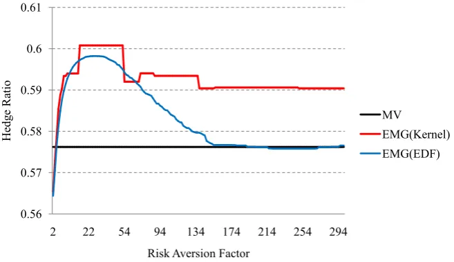
DOI: 10.4236/tel.2018.811162 2537 Theoretical Economics Letters = 2 to v = 300 are presented in Table 6. Meanwhile, Figure 3 provides a better illustration for EMG hedge ratios obtained from both estimation methods. It is clear from both illustrations that the hedge ratios estimated by kernel and EDF estimation methods share a few common characteristics. Some findings here are consistent with the results of EMG hedge ratios reported earlier, further justify-ing the robustness of the empirical results in this study.
First of all, the estimated EMG hedge ratios are significantly differ from the constant MVHR. The mean value for EMG hedge ratios is considerably greater than the MVHR. This indicates that investors would most probably severely un-der-hedged the CPO price risk with MVHR when the risk aversion is consi-dered. Second, investors with similar degree of risk aversion could have signifi-cantly different optimal futures positions. As the kernel hedge ratios function behaves like a step-function, the hedge ratios will experience momentous ‘jump’ at certain risk aversion parameter.
[image:18.595.209.538.517.707.2]Third, the hedge ratios become steadier as the risk aversion parameter in-creases. The hedge ratios for extremely risk averse investors (v > 100) tend to be more stable and nearly constant. However, these hedge ratios for higher risk aversion factors do not approach the MVHR. This is inconsistent with the EDF hedge ratios which approaches the MVHR for greater levels of risk aversion. Fourth, the kernel hedge ratios exhibit a nearly bell-like curve function. This finding verified the unique characteristic of the FCPO hedge ratio function dis-cussed earlier where the ratios experience a peak. Despite the results from both estimators share some similarities, noticeable differences do exist. Since the pri-mary objective here is to compare and contrast the hedge ratios obtained from both methods, Table 7 is constructed to highlight the differences between kernel and EDF hedge ratios. The empirical results reported in the following table sug-gest the hedge ratios estimated from the two mentioned methods are not equiv-alent. The table reveals that the kernel hedge ratios are typically larger than the EDF ratios.
Figure 3. EMG Hedge Ratios (Kernel and EDF Estimation Methods) for FCPO. 0.56
0.57 0.58 0.59 0.6 0.61
2 22 54 94 134 174 214 254 294
H
ed
ge R
at
io
Risk Aversion Factor
MV
DOI:10.4236/tel.2018.811162 2538 Theoretical Economics Letters Table 6. Kernel hedge ratios for various risk aversion parameters.
Risk Aversion
Factor EMG Hedge Ratio
EMG Coefficient for Unhedged
Portfolio
EMG Coefficient for Hedged
Portfolio
Hedging Effectiveness
MV 57.62 - - 42.40
EMG(a) 59.26 0.057198 0.045121 21.66
2 56.54 0.007854 0.005860 25.38 5 58.55 0.017043 0.012663 25.70 10 59.40 0.024651 0.018372 25.47 30 60.08 0.038802 0.029495 23.98 50 60.08 0.046359 0.035649 23.10 100 59.34 0.057418 0.044835 21.92 200 59.06 0.068748 0.054803 20.28 300 59.04 0.075243 0.060932 19.02 Note: (a) The hedge ratio and other items are calculated as the mean values of all estimated results.
Table 7. EMG hedge ratios by kernel and EDF estimation methods.
Risk Aversion
Factor Method EMG Hedge Ratio (%) Mean Portfolio Return (%)
EMG Coefficient for Hedged
Portfolio
Hedging Effectiveness
(%) Average Kernel 59.26 0.003812 0.0451213 21.66
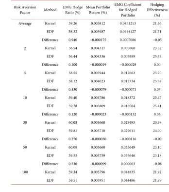
EDF 58.32 0.003987 0.0444127 21.71 Difference 0.940 −0.000175 0.0007086 −0.05 2 Kernel 56.54 0.004317 0.005860 25.38 EDF 56.44 0.004336 0.005889 25.38 Difference 0.100 −0.000019 −0.000029 0.00 5 Kernel 58.55 0.003944 0.012663 25.70
EDF 58.12 0.004023 0.012734 25.67 Difference 0.430 −0.000079 −0.000071 0.03 10 Kernel 59.40 0.003786 0.018372 25.47
EDF 59.28 0.003809 0.018504 25.41 Difference 0.120 −0.000023 −0.000132 0.06 30 Kernel 60.08 0.003660 0.029495 23.98
[image:19.595.187.536.339.734.2]DOI: 10.4236/tel.2018.811162 2539 Theoretical Economics Letters Continued
Difference 0.830 −0.000155 0.000349 −0.07 200 Kernel 59.06 0.003849 0.054803 20.28 EDF 57.63 0.004115 0.053666 20.36 Difference 1.430 −0.000266 0.001137 −0.08 300 Kernel 59.04 0.003853 0.060932 19.02 EDF 57.66 0.004109 0.058924 19.12 Difference 1.380 −0.000256 0.002008 −0.10 Note: (a) The differences are computed as the magnitude difference of kernel ratios in excess to EDF ratios.
It is clear and apparent from Figure 3 that although both kernel and EDF hedge ratios are almost identical for less risk averse investors, visible differences still occur. These similarities disappear and become substantial as the discre-pancy increases along with higher degree of risk aversion. Furthermore, thought with exceptions, the magnitude of the differences tends to be greater for higher risk aversion levels. The differences are larger than 100 basis points for extreme-ly risk averse investors (v > 100) with kernel hedge ratios take the greater ratios. However, the central issue remains whether which method offers better FCPO hedging performance.
In most cases, the EDF hedge ratios produce better hedging performance as measured by the hedging effectiveness. Nonetheless, one should note that the kernel hedge ratios outperformed the EDF hedge ratios for lower levels of risk aversion (v < 25). While EDF hedge ratios performs better for higher degree of risk aversion where the magnitude of the differences increases with risk aversion factor. Although the difference between the hedging effectiveness of kernel and EDF hedge ratios are notable, there are less pronounced as the highest magni-tude difference (v = 300) is 10 basis points which is very minimal. In addition, the kernel hedge ratios generally create portfolio with lesser returns than the EDF hedge ratios. This is due to the higher hedge ratios of the kernel method which requires shorting more FCPO contracts, thus lowering the yield on the bullish CPO market.
These results provide insights suggest that the EDF method is more effective and gives better hedging performance than the kernel method in the Malaysian CPO markets. The superior performance of EDF estimation method is demon-strated based on the in-sample tests performed. One would expects the more powerful kernel estimation method will provide better results and performance than the less efficient EDF estimation method, however the empirical results are contradictory. The EDF method performs equally well to the more powerful and efficient kernel method.
DOI:10.4236/tel.2018.811162 2540 Theoretical Economics Letters of kernel estimation method does not translate its statistical advantages into bet-ter hedging performance. Hence, the kernel and EDF methods would produce almost identical hedging performance for the CPO market. It is therefore be-lieved that the EDF estimator could performs at least equally well to the kernel estimator for a very large sample size.
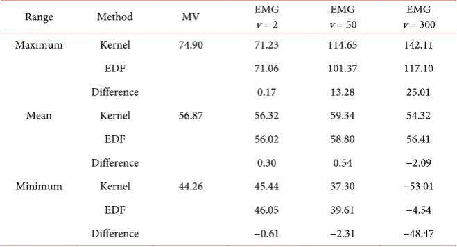
3.5. The Dynamic Hedge Ratios by Moving Data Window
As far as this, the empirical findings discussed above were based on the ‘buy and hold’ strategy where considerations only given to the constant hedge ratios for the whole sample period. Here, the study extends the empirical application by considering the case where the hedgers re-evaluate the hedge ratios continually. Indeed, hedgers and investors might want to adjust their hedging strategy accor-dingly to new available information. Following Hodgson and Okunev [14], Kolb and Okunev [15] and Lien and Luo [16], moving data windows which consist of 500 data points are applied to investigate the stability of the optimal hedge ra-tios. In aggregate, the rolling window moves across observations will produce 3422 hedge ratios for a given risk aversion factor; the EMG dynamic hedge ra-tios. These dynamic hedge ratios will then be examined by comparing the mag-nitude of changes of consecutive hedge ratios.
For comparison purposes, the MVHR and the EMG hedge ratios for three risk aversion parameter, v = 2, v = 50 and v = 300 which represent low, moderate and highly risk averse investors respectively are estimated. Table 8 reports the sum-mary of the empirical results for the dynamic hedge ratios of parameter v = 2, v
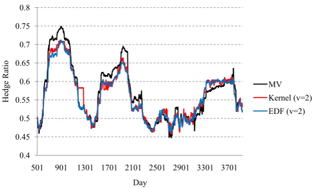
[image:21.595.212.539.512.706.2]= 50 and v = 300. The dynamic hedge ratios for low risk aversion factor (v = 2) follow closely the same path as the dynamic MVHR (Figure 4). These dynamic hedge ratios are trending in the same manner across the sample period with mild variations. However, it should be noted that gradual changes do occur fre-quently. Despite so, in retrospect, noticeable changes in dynamic hedge ratios happen occasionally where the range for MVHR is between 44.26% and 74.90%.
Figure 4. EMG Dynamic Hedge Ratios for Risk Aversion Factor, v = 2.
0.4 0.45 0.5 0.55 0.6 0.65 0.7 0.75 0.8
501 901 1301 1701 2101 2501 2901 3301 3701
H
ed
ge R
at
io
Day
DOI: 10.4236/tel.2018.811162 2541 Theoretical Economics Letters Table 8. Summary of the dynamic hedge ratios for FCPO.
Range Method MV EMG v = 2 v = 50 EMG v = 300 EMG
Maximum Kernel 74.90 71.23 114.65 142.11
EDF 71.06 101.37 117.10
Difference 0.17 13.28 25.01 Mean Kernel 56.87 56.32 59.34 54.32
EDF 56.02 58.80 56.41
Difference 0.30 0.54 −2.09 Minimum Kernel 44.26 45.44 37.30 −53.01
EDF 46.05 39.61 −4.54
Difference −0.61 −2.31 −48.47 Note: (a) The difference is denoted as the excess of kernel hedge ratio to the EDF hedge ratio. (b) Negative hedge ratio indicates buying FCPO contracts to hedge against the price risk instead of shorting the FCPO contracts.
Meanwhile, it appears that the MV approach is comparatively more stable than the EMG approach for CPO market. This is particularly evident from the maximum and minimum of EMG hedge ratios for greater degree of risk aver-sion investors. The dynamic hedge ratios for higher risk averaver-sion factor (v = 300) have greater volatility than less risk averse investors. It could be observed from Figure 5 and Figure 6 where the dynamic hedge ratios for moderate (v = 50) and highly (v = 300) risk averse investors fluctuated well above and below the dynamic MVHR. Also, the estimated kernel and EDF dynamic hedge ratios for highly risk averse investors follow step function. This indicates that the subs-titution of an obsolete data point by the newest as the data window moves could results a drastic change in optimal hedge ratios.
Moreover, another interesting result is the optimal EMG hedge ratios take values greater than 100% and less than 0% occasionally during the sample period for more risk averse investors. A hedge ratio which is greater than 100% implies the hedger should hedge more than the spot CPO position taken. A possible ex-planation is the backwardation of the CPO market itself [15]. A backwardated market exhibits weak links between the spot and futures prices as explained by the theory of storage. Hence, the hedgers would need to hedge more than the exposed price risk. On the other hand, a negative hedge ratio indicates the hedg-ers should long FCPO contracts rather than shorting it. It is observed that these estimated negative hedge ratios take place during adverse economic conditions, particularly during 2000-2001 dot-com bubbles and sub-prime mortgage crisis started in 2006. Therefore, having long position on FCPO during economic downturns will then generates lucrative profits when economy recovers; similar to the so called “buy low sell high” investment strategy.
DOI:10.4236/tel.2018.811162 2542 Theoretical Economics Letters
[image:23.595.216.533.285.478.2]Figure 5. EMG Dynamic Hedge Ratios for Risk Aversion Factor, v = 50.
Figure 6. EMG Dynamic Hedge Ratios for Risk Aversion Factor, v = 300.
and obvious for strongly risk averse (v = 300) investors where the hedge ratios could differ considerably. The magnitude differences are typically arising from the method used to generate the hedge ratio series. This is consistent with the earlier findings where kernel and EDF estimates generally produce noticeably difference hedge ratios especially for greater risk aversion factor. These observa-tions are strengthened when the magnitude changes of consecutive hedge ratios are being considered.
Table 9 depicts the absolute differences of consecutive dynamic hedge ratios. The results here reinforce earlier observations when examining the stability of hedge ratios. As noted before, moderate and highly risk averse investors have dynamic hedge ratios which are more volatile over time. With reference to the following table, the changes in consecutive hedge ratios are less than 5% for MV practitioners or investors with low level of risk aversion (v = 2). However, gra-dual variation occurs more frequently than higher risk averse investors.
0.35 0.45 0.55 0.65 0.75 0.85 0.95 1.05 1.15
501 901 1301 1701 2101 2501 2901 3301 3701
H
ed
ge R
at
io
Day
MV
Kernel (v=50) EDF (v=50)
-0.55 -0.35 -0.15 0.05 0.25 0.45 0.65 0.85 1.05 1.25 1.45
501 901 1301 1701 2101 2501 2901 3301 3701
H
ed
ge R
at
io
Day
MV
DOI: 10.4236/tel.2018.811162 2543 Theoretical Economics Letters Table 9. Absolute consecutive changes in hedge ratios for FCPO.
Range (%)(a) MV EMG
(v = 2) (v = 50) EMG (v = 300) EMG Kernel EDF Kernel EDF Kernel EDF (0, 0.05) 1474 1966 1091 1946 2276 2062 3165 (0.05, 0.10) 627 281 607 228 254 352 20 (0.10, 0.50) 1079 715 1525 674 646 724 40 (0.50, 1.00) 166 303 176 282 101 160 53 (1.00, 5.00) 75 156 22 226 116 90 92 (5.00, 10.00) 0 0 0 55 25 10 26 (10.00, 50.00) 0 0 0 10 3 18 24 (50.00, 100.00) 0 0 0 0 0 4 1
(100.00, ∞) 0 0 0 0 0 1 0
Note: (a) The numbers in (a, b) indicate the lower and upper bounds on the hedge ratio changes respec-tively where the unit measure is percentage.
Conversely, the dynamic hedge ratios for moderate and highly risk averse in-vestors record greater magnitude change. Although infrequent, some of these changes affect the optimal hedge ratios by a magnitude of 10% or more. Also, the dynamic hedge ratios for higher risk aversion levels contain constant or nearly constant hedge ratios with minimal absolute changes more regularly than lower risk aversion factors. This is reflected in Table 9 where the absolute con-secutive changes for the range between 0% and 0.05% records highest frequency for strongly risk averse investors.
The inertia of substantial changes in hedge ratio for higher value of risk aver-sion parameter constitute to the instability of the dynamic hedge ratio. These significant changes are caused by the multiple-root problem in solving the esti-mating function [16]. Multiple roots exist when a mathematical expression is raised to higher power. In the case of highly risk averse investors (v = 300), the EMG method has more than one root implying multiple local minimum. As data window moves across observation where one data point is being replaced by another, it happens that one local minima replaces another as the global mini-mum. Hence, it explains the momentous ‘jump’ that causes instability in the dy-namic hedge ratios.
DOI:10.4236/tel.2018.811162 2544 Theoretical Economics Letters their interest.
To summarize, the EMG hedge ratios obtained from both kernel and EDF es-timator are generally differ from the estimated MVHR of the MV approach. It is also evident that kernel and EDF methods produce noticeably different optimal hedge ratios while yielding similar hedging performance. It is therefore argued that the less efficient EDF estimation method would performs equally to the more powerful kernel estimation method for large sample. Besides, the empirical evidence shows the instability of both MVHR and EMG hedge ratios over time where optimal hedge ratios for higher degree of risk aversion record the greatest variation. In short, investors with heterogeneous risk attitudes should exercise care as the optimal hedge ratios are sensitive to risk aversion parameter and in-stable over different time horizons.
4. Conclusions
The attractive feature of Extended Mean-Gini (EMG) is credited to its revoca-tion of the distriburevoca-tional assumprevoca-tions of normality and its consistency with second order of stochastic dominance. The non-normality returns of Malaysian Crude Palm Oil (CPO) and CPO Futures (FCPO) evidently inspires sound mo-tivation for stochastic dominance model. This paper presents EMG framework as an alternative approach for futures hedging in Malaysian CPO market. It thereby captured the observed diversity of risk behavior in futures hedging. The constant and time-varying dynamic hedge ratios are computed by the Empirical Distribution Function (EDF) estimation method and the more effi-cient non-parametric Kernel estimation method. The hedging performance is then being compared by assessing the hedging effectiveness of each estimation method. Furthermore, the investigations of the stability of optimal hedge ratios are conducted.
Consistent with the results of Cheung et al. [26]; Hodgson and Okunev [14]; Kolb and Okunev [15]; Shaffer and DeMaskey [32]; Butterworth and Holmes
[33], the EMG hedge ratios are substantially different from the traditional Min-imum-Variance hedge ratio (MVHR) for various classes of risk averse investors. Investors who rely on the MVHR to optimally hedge the CPO spot position may be misguided and therefore mishedged the risk exposure. Overall results show the MVHR is generally more favorable and applicable for highly risk averse in-vestor despite minima differences are observed. However, it is inappropriate for low and moderate risk averse investors whereas the degree of mishedged is higher as compared to highly risk averse hedgers.
DOI: 10.4236/tel.2018.811162 2545 Theoretical Economics Letters their spot position.
Furthermore, the empirical results show the EMG hedge ratios estimated by the EDF and kernel estimations methods are indeed different. This is consistent with the findings of Shaffer [29] and Shaffer and DeMaskey [28]. The study con-firms that the kernel hedge ratios are greater than EDF hedge ratios on average. However, the kernel hedge ratios generally do not produce better hedging per-formance than EDF hedge ratios in FCPO hedging. Given a large sample size, the efficiency of a more powerful kernel estimation method has failed to provide improvement to the hedging performance. It is argued that the efficiency of kernel method is not evident for large sample size. Conversely, the simpler EDF estimation method performs reasonably well with large sample and generally over-performed the kernel estimation method. Overall, the empirical findings favor the EDF estimation method for the CPO and FCPO markets.
Meanwhile, it is found that the EMG hedge ratio is a bell-like curve function with respect to risk aversion factor. Both kernel and EDF hedge ratios exhibit asymmetric bell-like curve with EDF hedge ratios being a smooth function while kernel hedge ratios follow a step function. The hedge ratio is neither a mono-tonically increasing nor decreasing function, contrary to the conclusions of Hodgson and Okunev [14]; Kolb and Okunev [15] Lien and Luo [16]; Butter-worth and Holmes [33]. This unique characteristic is influenced by the supply and demand dynamics of CPO and the investors’ risk aversion attitudes of high-er prefhigh-erences on return.
This paper also demonstrates that the dynamic hedge ratios for moderate and highly risk averse investors are considerably more volatile than low level of risk aversion investors. These results are very much consistent with the findings of Hodgson and Okunev [14]; Kolb and Okunev [15]; Lien and Luo [16]. As a con-sequence, investors of higher risk aversion levels who adopt “buy and hold” strategy will face the risk of significantly mishedged the portfolio. Since the vola-tility of dynamic hedge ratios for low risk averse and MVHR reliance investors are lesser, they still run the risk of significantly mishedged the portfolio although at a slighter tendency. Following Lien and Luo [16], the instability of EMG hedge ratio is constituted by the multiple-root problem where multiple local mi-nima exist in solving the estimation. This leads to the step function of dynamic hedge ratios for moderate and highly risk averse investors.
DOI:10.4236/tel.2018.811162 2546 Theoretical Economics Letters One important limitation of EMG approach is the absolute risk aversion in-terval represented by the user-predetermined parameter v in EMG approach is not known exactly [37] [38]. According to McDonald et al.’s [38] assertion, the utilization of the EMG method did not provide an exact range for the risk aver-sion parameter. Consequently, it is possible to underestimate or overestimates the degree of risk aversion in EMG analysis. This shortcoming renders the mag-nitudes of risk aversion not directly comparable across studies of various frameworks. Hence, preventing one from the performance assessment of EMG approach in futures hedging. Therefore, in order to assess the hedging perfor-mance of EMG approach, it is important to convert the existing risk aversion parameter into a common measure. By doing so, the effectiveness of EMG ap-proach could be compared with other models which considered risk aversion factor in hedging. Despite so, the estimation of absolute risk aversion is subject to sampling error while cross-study comparisons are often difficult to apply [37]. However, the questions remain unanswered in this paper is open for future research: does out-of-sample analysis yield the same results as discussed pre-viously? Is EMG approach a better model to quantify risk aversion in futures hedging? Though many questions around EMG approach are left unanswered, the EMG framework still appears to be a promising framework than the conven-tional mean-variance approach. Furthermore, futures researches of FCPO hedg-ing on Malaysia’s FCPO market are greatly encouraged as the literature re-sources of hedging effectiveness in Malaysia CPO and FCPO markets are very limited.
The empirical findings of this research is particularly important and essential for parties who are involve in the CPO market, such as the CPO investors, fund managers, financial practitioners, regulators and the academic community. Through the results, the EMG framework is demonstrated as more superior and promising than the traditional Mean-Variance framework. CPO Investors or hedgers could employ this framework to optimally hedge the CPO exposure ex-clusive of the normality assumptions. The main econometric advantage of EMG approach is its efficiency implies second-order of stochastic dominance which requires only the first absolute moment. Furthermore, it offers the simplicity to incorporate the risk aversion factor where investors could hedge their CPO portfolio accordingly to their risk behavior.
With respect to the findings, the EDF estimation method appears to be a bet-ter option to estimate EMG coefficient when a large sample is considered. In-vestors are able to estimate hedge ratios for a given degree of risk aversion at a shorter time with EDF method. Since the simpler rank-based estimation per-forms equally well with the kernel-based estimator, investors should probably opt for EDF hedge ratios when sample size is large. However, hedgers who wish to adopt EMG approach are advised to exercise great care when choosing the risk aversion parameter.