A Logarithmic Complexity Algorithm for Nearest Neighbor Classification Using Layered Range Trees

http://dx.doi.org/10.4236/iim.2012.42006 Published Online March 2012 (http://www.SciRP.org/journal/iim)

A Logarithmic-Complexity Algorithm for Nearest

Neighbor Classification Using Layered Range Trees

Ibrahim Al-Bluwi1, Ashraf Elnagar2

1

Laboratory for Analysis and Architecture of Systems (LAAS-CNRS), Universitt’e de Toulouse, Toulouse, France

2

Department of Computer Science, University of Sharjah, Sharjah, UAE Email: ashraf@sharjah.ac.ae

Received November 25, 2011; revised December 27, 2011; accepted January 5,2012

ABSTRACT

Finding Nearest Neighbors efficiently is crucial to the design of any nearest neighbor classifier. This paper shows how Layered Range Trees (LRT) could be utilized for efficient nearest neighbor classification. The presented algorithm is robust and finds the nearest neighbor in a logarithmic order. The proposed algorithm reports the nearest neighbor in , where k is a very small constant when compared with the dataset size n and d is the number

of dimensions. Experimental results demonstrate the efficiency of the proposed algorithm.





log logd

O d2 n  nkd

Keywords: Nearest Neighbor Classifier; Range Trees; Logarithmic Order

1. Introduction

Nearest Neighbor Classifiers enjoy good popularity, and have been widely used since their introduction in 1967, [1]. The simplest form of Nearest Neighbor (NN) classi- fication works as follows: Given a set of labeled training examples, a query instance is given the same label as that of the most similar example(s) in the training set. It has been shown in [1] that nearest neighbor classification pro- duces correct results with an error rate that is less than twice the error of the most sophisticated classification technique given the same information. This simple error bound, as well as the overall simplicity of the method, its intuitive- ness, and its capability of learning complex functions without the need of any training are mainly what have made it an attractive classification technique.

One of the most important difficulties that face NN classification is the classification speed. That is, the time the classifier takes to find the nearest neighbor(s) to the query instance. A naive NN finding algorithm would iterate through all of the dataset, measure the distance between the query instance and every other instance in the data set, and then determine the nearest neighbor(s) accordingly. Clearly this requires O (dn) time, where n is the number of records in the dataset and d is the number of attributes (dimensions) in each record. As mentioned before, this is time consuming and may be intractable when n is large and d is high. Recent works such as adopting mutual nearest neighbors instead of k nearest neighbors to clas- sify unknown instances lead to better performance [2,3].

In order to overcome the slow execution speed and high storage requirements (when dealing with large datasets), several recent research attempts were reported in the lit- erature such as assigning weights to training instances [4] and using probabilistic variant of the partial distance search- ing in low dimensions [5]. Using the condense approach [6] to remove patterns that are more of a computational burden to lead to better classification accuracy.

Finding nearest neighbors is not only a classification problem but it is related to many diverse fields, and there- fore the performance bottleneck is an issue. Thus, consider- able work has been done and is still going on for efficient NN finding techniques. Such techniques could be grouped into a number of broad range categories, the most relevant of which is the category of techniques which are based on space partitioning.

An example of such techniques is the use of Voronoi Diagrams. Finding the nearest neighbor based on a Vo- ronoi Diagram can be done in logarithmic time, however, constructing and storing a Voronoi Diagram grows ex- ponentially with the number of dimensions, [7].

similar to K-d Trees and have a similar NN performance. However, they address some of the problems inherent in K-d Trees. R-Trees are optimized for I/O access, their space partitioning suits multimedia applications, and their per- formance does not deteriorate after performing updates.

The Layered Range Tree (LRT) [11,12] is another space partitioning data structure, which supports Orthogonal Range Queries in _O





time, where d, is the number of dimensions, n is the number of points, and k is the number of reported points. This outmatches the per- formance of the other main-memory range querying data structures like the K-d Tree. This paper shows how the LRT can be used as a classifier that finds nearest neighbors in a logarithmic order.

The remainder of this paper is organized as follows: Sec- tion 2 describes the layered range tree and its basic con- struction and range querying algorithms. Section 3 ex- plains the LRT nearest neighbor classification algorithm and Section 4 discusses and analyzes its complexity and shows some results. Finally, conclusions and future work directions are outlined in Section 5.

2. The Layered Range Tree

The LRT was first described by Willard [12] and Lueker [12]. It is a multi-dimensional data structure that supports multidimensional Orthogonal Range Queries in





logd

O  nk time, where d is the number of dimen- sions, n is the number of points, and k is the number of reported points.

To understand the LRT, we first describe the Range Tree. A 2d range tree is a binary search tree (BST), where every node in the tree has an associated structure con-nected to it. This tree is said to have two levels. The first level is the first main BST, and the second level is the associated structures that are connected to the nodes of the first level. Hence, a range tree for a set of 3-dimen- sional points would have three levels, where the third level is made up of associated structures that are con- nected to every node in every associated structure in the second level.

Given a set of points S, the first (main) BST in the LRT is built using the x-coordinate of S. This allows doing binary searches for points in S using the x-coordi- nate only. The associated structure to any node in the main BST contains all points that lie under that node in the tree, but sorted using the second dimension, the y-coor- dinate. Therefore, the associated structure of the root node (of the first BST) contains all points in S sorted according to y. Figure 1 depicts a 2d range tree. Both the shaded areas represent trees that have the same set of points. However, the one in the main tree is sorted ac- cording to x whereas the associated tree is sorted based on y. Each node in the main tree has such an associated tree.

The LRT goes one step further than the range tree by applying the technique known as fractional cascading [13], which speeds up the search process by eliminating binary searches that should be done at level d (e.g., at level 2 in a 2-dimensional set of points). Figure 2 illus-trates the LRT with its second level structures connected using fractional cascading.

When an array is connected to another array using frac- tional cascading, every node in the first array is connected to the first node in the second array that is greater than or equal to it. If there is no such node, the link is nullified. For illustration, consider Figure 2, every node in the associ- ated array of v is connected to at most two nodes that are larger than or equal to it; one from the associated array of L and the other from the associated array of R.

Given an LRT and two points (x1, y1) and (x2, y2), an-

swering the range query [x1: x2] × [y1 : y2] proceeds as fol-

lows. A binary search is first carried out on the main tree to find the node whose x value lies between x1 and x2.

This node is called the split node. Next, another binary search is repeated for y1 at the associated structure of the

split node. As descending the main tree, to search for points that lie between x1 and x2, the associated arrays are de-

scended following the pointers. For example, if the left child of the split node is visited, the pointer between y1 in

the associated tree of the split node and the associated array of the left child of the split node is traversed. If a node which lies in the [x1: x2] range is reached then there is no

Range Tree

Associated Tree

Figure 1. A 2d range tree.

V

L R

need to do a binary search for y1 in its’ associated tree as

it was traced while descending. A walk from y1 to y2 is

then performed to report the points.

In NN classification as well as in other applications, search may not have to proceed in all dimensions. With the current structure of the LRT, stopping at a dimension that is less than d means that we will not be able to make use of fractional cascading in improving the query time. Therefore, the LRT can be built such that fractional cas- cading links are built for all dimensions rather than just the last one. Furthermore, in order to enable walking in the associated trees, all leaves in every tree should be con- nected using pointers (Figure 3).

3. Classifying Using the LRT

In a dataset, instances with d attributes could be looked at as points in d dimensional space. When searching for near- est neighbors to a query point q, it would be effective if we could search only points that surround q, and avoid searching parts of the space that are far from q. The idea of the discussed algorithm is simply to reduce the NN find- ing problem to a range query that returns a relatively small set of points (instances) that surround q. This small set can then be searched for the nearest neighbor quickly using brute force.

Since a range query using the LRT is known to be ef- ficient, the key issue becomes to find a suitable range query interval that contains only points that are adjacent to q and that are likely to have the nearest neighbor. The less the number of these points is, the better the performance is, and the larger it is the closer the performance becomes to exhaustive search.

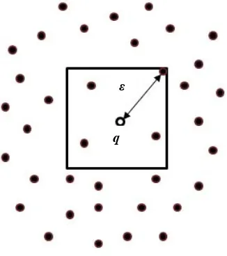
Figure 4 illustrates the idea of the algorithm in a 2d space. The algorithm first finds a suitable and uses it to build a query range [limit1: limit2] around q. After choosing

, the interval [limit1: limit2] could be built (for example)

as follows:





,

d

d

q 

  _{ }

, +

d

d

q

 

  

 

1 2

1 d , ,d

limit _q  q 

1 2

2 d+ , + ,d

limit  q  q 

Next, the LRT can be used to retrieve all points that lie within that range, and then do an exhaustive search for the nearest neighbor among these retrieved points.

In order to achieve efficient results, the number of points retrieved from the range query must be small when com- pared to the number of points in the dataset. If the num- ber of retrieved points is large, there would be no con- siderable benefit over using exhaustive search. Therefore, $/epsilon$ must be chosen carefully since it is what de-fines the range around q.

There are several ways to determine . A probabilistic method is presented in [14] to find in constant time. In our implementation of the algorithm, we have used a

Figure 3. A multidimensional layered range tree.

ε

q

 





 





logd

O n  n

 

Figure 4. An example of q and in a 2d space.

logarithmic-time heuristic to approximate . This heu- ristic gives a good approximation for , on average and guarantees that there will always be at least one point in the retrieved set.

The heuristic estimates by doing a binary search in the data set for q in every dimension. That is, a search for q is firstly done using d1, then another binary search is

done using d2, and so on. As the binary search proceeds,

the distance between any visited point and q is measured and is updated to hold the minimum distance found so far. The reason behind adopting this strategy is that on the search path for q, close points to q are likely to be visited. The closer the search gets to q in one dimension the smaller the upper bound for the distance to the nearest neighbor is made. How effective is this method? This is discussed in details in the next section.

4. Algorithm Analysis and Discussion

Constructing the LRT can be done in

time and it requires O n





 

storage. On the other hand, issuing a range query on an LRT is of order

The proposed algorithm is made up of three parts: finding , issuing the range query, and searching the retrieved points. The overall complexity of the algorithm if the aforementioned heuristic is used is:







2_log

d n



log

d n

d 1

log  n

log

d nk

2_log

O d n , where k is a number that is

small on average and that is more likely to be larger if the number of dimensions is large.

The term is due to the binary searches done to find . The heuristic does d binary searches; every binary search costs in the worst case since com- paring two instances constitutes comparing d attributes. The part comes from the range query done using the LRT as described before. Finally, the kd term is the number of distance measures done in the last brute force step done on the points retrieved from the range query. Therefore, the total number of distance measures done is

compared to n if brute force was used. To test the performance of the algorithm and see how large k is on average for every dimension, we performed two tests. The first was done on randomly generated datasets for dimensions 1 - 7. The size of every data set was 100, and for each data set the NN query was re- peated 100 times and the average finding time was re- corded for every dimension. Since 100 is relatively small, the test was repeated 100 times and the average of these 100 repetitions was recorded for both the LRT and the brute force algorithms. The results are depicted in Fig-ures 5 and 6.

The second test was done on 4 standard datasets: The

Figure 5. Performance in time between LRT NN and BF algorithms on the synthetic dataset.

Figure 6. Performance in comparisons between LRT NN and BF algorithms on the synthetic dataset.

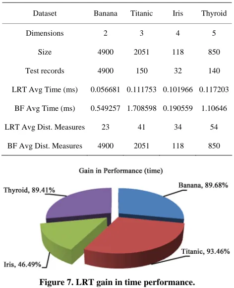
Banana dataset1, Titanic dataset2, Iris dataset3 and Thy- roid dataset4. Table 1 shows the dimension of every dataset, its size and shows how the proposed algorithm performs on it compared to exhaustive search. Figure 7 depicts the significant overall gain in time performance of LRT over BF.

Looking at Figures 5 and 6 in addition to Table 1, it is clear that the algorithm performs very well in dimensions less than 7. Testing with dimensions more than 7 was not easy due to memory constraints, since the implemented LRT loads all records into memory. When the data set is large and when the number of dimensions is high, load- ing the whole data set to memory is not possible, and since we are dealing with data mining problems, it is very likely to have huge datasets. Therefore, converting the LRT into an index structure becomes a normal procedure. The question that poses itself is: will the LRT perform equally good when converted to an index structure?

In main memory, the most expensive operation was the distance measure, and therefore, we considered it in our tests. However, when the records are all in a file, the most expensive operation becomes the I/O done to access a record. Therefore, the performance measure is changed.

Table 1. The performance of the LRT NN algorithm on four datasets.

Dataset Banana Titanic Iris Thyroid

Dimensions 2 3 4 5

Size 4900 2051 118 850

Test records 4900 150 32 140

LRT Avg Time (ms) 0.056681 0.111753 0.101966 0.117203

BF Avg Time (ms) 0.549257 1.708598 0.190559 1.10646

LRT Avg Dist. Measures 23 41 34 54

BF Avg Dist. Measures 4900 2051 118 850

Figure 7. LRT gain in time performance.

1_{http://ida.first.fraunhofer.de/projects/bench/benchmarks.html}

2_{http://www.cs.toronto.edu/~delve/data/titanic/desc.html}

3_{http://mlearn.ics.uci.edu/databases/iris/}

1

logd n





ogd n kd

 

log

d n k

After changing the LRT to an index structure, it showed that it no more performed as well as it used to do in main memory since became the dominant term. One way to overcome this is to convert the Binary Search Trees in the LRT to B-Trees, which are optimized for I/O access.

5. Conclusion and Future Work

In this paper, a simple and efficient algorithm for nearest neighbor classification was presented. The algorithm is based on the Layered Range Trees. It converts the near- est neighbor query into a range query that is answered efficiently, and that returns a small number of instances that are searched for the nearest neighbor. The presented algorithm finds the nearest neighbor in

2

log l

O d n , where k is a number that is

small on average and that is more likely to be larger if the number of dimensions is large. The number of dis- tance measures done by the algorithm is  . Future work will focus on optimizing the way the nearest neighbor query is converted to a range query, as well as optimizing the algorithm to handle large datasets and high dimensional data.

REFERENCES

[1] T. Cover and P. Hart, “Nearest Neighbor Pattern Classi-fication,” IEEE Transactions on Information Theory, Vol. 13, No. 1, 1967, pp. 21-27.

doi:10.1109/TIT.1967.1053964

[2] Y. Gao, B. Zheng, G. Chen, Q. Li, C. Chen and G. Chen, “Efficient Mutual Nearest Neighbor Query Processing for Moving Object Trajectorie,” Information Sciences, Vol. 180, No. 11, 2010, pp. 2176-2195.

doi:10.1016/j.ins.2010.02.010

[3] H. W. Liu, S. C. Zhang, J. M. Zhao, X. F. Zhao and Y. C. Mo, “A New Classification Algorithm Using Mutual Nearest Neighbors,” 9th International Conference on Grid and Cooperative Computing (GCC), Nanjing, 1-5 November 2010, pp. 52-57.

[4] M. Z. Jahromi, E. Parvinnia and R. John, “A Method of Learning Weighted Similarity Function to Improve the Performance of Nearest Neighbor,” Information Sciences, Vol. 179, No. 17, 2009, pp. 2964-2973.

doi:10.1016/j.ins.2009.04.012

[5] J. Toyama, M. Kudo and H. Imai, “Probably Correct

k-Nearest Neighbor Search in High Dimensions,” Pattern Recognition, Vol. 43, No. 4, 2010, pp. 1361-1372. doi:10.1016/j.patcog.2009.09.026

[6] H. A. Fayed and A. F. Atiya, “A Novel Template Reduc-tion Approach for the k-Nearest Neighbor Method,”IEEE Transactions on Neural Networks, Vol. 20, No. 5, 2009, pp. 890-896. doi:10.1109/TNN.2009.2018547

[7] F. P. Preparata and M. I. Shamos, “Computational Ge-ometry: An Introduction,” Springer, Berlin, 1985. [8] J. L. Bentley, “Multidimensional Binary Search Trees

Used for Associative Searching,” Communications of ACM, Vol. 18, No. 9, 1975, pp. 509-517.

doi:10.1145/361002.361007

[9] A. Guttman, “R-Trees: A Dynamic Index Structure for Spatial Searching,” SIGMOD’84 Proceedings of the 1984

ACM SIGMOD International Conference on Management of Data, Vol. 14, No. 2, 1984, pp. 47-57.

[10] J. H. Freidman, J. L. Bentley and R. A. Finkel, “An Algo-rithm for Finding Best Matches in LogaAlgo-rithmic Expected Time,” ACM Transactions on Mathematical Software

(TOMS), Vol. 3, No. 3, 1977, pp. 209-226. doi:10.1145/355744.355745

[11] G. S. Lueker, “A Data Structure for Orthogonal Range Queries,” Proceedings of the 19th Annual IEEE Sympo-sium on Foundations of Computer Science, Ann Arbor, 16-18 October 1978, pp. 28-34.

[12] D. E. Willard, “New Data Structures for Orthogonal Range Queries,” SIAM Journal on Computing, Vol. 14, No. 1, 1985, pp. 232-253. doi:10.1137/0214019

[13] B. Chazelle and L. J. Guibas, “Fractional Cascading: A Data Structuring Technique with Geometric Applica-tions,” Proceedings of the 12th Colloquium on Automata,

Languages and Programming, Vol. 194, 1985, pp. 9-100. doi:10.1007/BFb0015734

[14] S. A. Nene and S. K. Nayar, “A Simple Algorithm for Nearest Neighbor Search in High Dimensions,” IEEE Transactions on Pattern Analysis and Machine Intelli-gence, Vol. 19, No. 9, 1997, pp. 989-1003.

doi:10.1109/34.615448