Abstract— Perishable inventory constitute a large portion of the world economy and include virtually all foodstuffs, pharmaceuticals, fashion goods, electronic items, periodicals, digital goods and many more as they lose value with time due to deterioration and/or obsolescence. Retailers dealing with perishable goods have to consider the factors of short shelf life and the dependency of sales volume on the amount of inventory displayed in determining optimal procurement policy. This paper presents an inventory model for continuously deteriorating goods having random shelf life and displayed inventory dependent demand. The model relaxes condition of zero stock at the end of cycle and maintains reserve stock to stimulate the demand. Under standard assumptions of single product, instantaneous replenishment with zero lead time, and constant deterioration rate; Economic Order Quantity (EOQ) is determined for maximizing profit. Computational results of numerical example suggest that profit decreases with reserve inventory; deterioration rate has pronounced impact on order quantity and profit as compared to inventory dependent demand factor. Sensitivity analysis of the model is also reported.
Keywords— Retail Inventory, Perishable Goods, Inventory
Dependent Demand, EOQ
I. INTRODUCTION
OST of the inventory models in the literature are based on assumption of imperishability of goods with infinite useful life. However, there are many goods that either deteriorate and/or become obsolete in the course of time and such perishable goods require different modelling. Retailers dealing with perishable goods have to consider factors of short shelf life and the dependency of sales volume on the amount of inventory displayed in determining optimal procurement policy.
Perishable inventory forms a large portion of total inventory and include virtually all foodstuffs, pharmaceuticals, fashion goods, electronic items, periodicals (newspapers/magazines), digital goods (computer software, video games, DVD) and many more as they lose value with time due to deterioration and/ or obsolescence. Perishable goods can be broadly classified into two main categories based on: (i) Deterioration (ii) Obsolescence.
Manuscript received on December 31, 2011; revised on January 25, 2012. This work was supported in part by IRCC, IIT Bombay under Grant 08IRCC037.
Madhukar Nagare is a research scholar at SJM School of Management, Indian Institute of Technology, Bombay, Mumbai-400076, India (e-mail: [email protected]).
Pankaj Dutta is an Assistant Professor in SJM School of Management, Indian Institute of Technology, Bombay, Mumbai-400076, India (corresponding author, Tel.: (+91) 22 25767783, e-mail: [email protected]).
Deterioration refers to damage, spoilage, vaporization, depletion, decay (e.g. radioactive substances), degradation (e.g. electronic components) and loss of potency (e.g. pharmaceuticals and chemicals) of goods. Obsolescence is loss of value of a product due arrival of new and better product [1]. Perishable goods have continuous or discrete loss of utility and therefore can have either fixed life or random life. Fixed life perishable products have a deterministic, known and definite shelf life and examples of such goods are pharmaceuticals, consumer packed goods and photographic films. On the other hand, random life perishable products have a shelf life that is not known in advance and variable depending on variety factors including storage atmosphere. Items are discarded when they spoil and the time to spoilage is uncertain. For example, fruits, vegetables, dairy products, bakery products etc., have random life [2].
It is found that for some goods, demand rate is directly related to the amount of inventory displayed in the retail store. Wolfe [3] provided empirical evidence that sales of style merchandise, like women’s dresses or sports clothes, is proportional to the amount of inventory displayed. Levin et al. [4] reported that retail sales is proportional to inventory level and a large pile of goods displayed would lead the customers to buy more. Silver and Peterson [5] found that the retail sales is proportional to the inventory displayed. These observations have attracted the attention of many researchers and practitioners to investigate the situation where the demand rate is dependent on inventory level in a store. Gupta and Vrat [6] developed an inventory model where demand rate is dependent on initial stock-level ( rather than instantaneous inventory level). Baker and Urban [7] was the first one to develop model with the idea of diminishing demand rate along with stock-level throughout the cycle. Datta and Pal [8] modified the concept of Baker and Urban with assumption that demand rate would decline with inventory up to a certain level, and then remain constant for the rest of the cycle and cycle terminates with zero stock. In their later formulation, Padmanabhan and Vrat [9] used selling rate dependent on current inventory with backlogging. Soni and Shah [10] formulated optimal ordering policies model for retailer where demand is partly dependent on stock with credit facility to retailer.
Prior studies assumed that cycle ending inventory as zero but noting the positive relation between revenue and higher inventory levels, Urban [11] relaxed the terminal conditions of zero ending inventories. Larson and DeMarais [12] referred the displayed inventory that stimulate the demand as ‘psychic stock’ and suggested ‘full-shelf merchandising’ policy i.e. display area be always kept fully stocked to
Madhukar Nagare and Pankaj Dutta
Continuous Review Model for Perishable
Products with Inventory Dependent Demand
increase sale. Smith and Achabal [13] refer to this stock as “fixtures fill” inventory which is considered as minimum on-hand inventory for adequate presentation by a retailer. This paper treats this inventory as reserve inventory.
The purpose of this paper is to find an optimal procurement policy for a retailer that deals with continuously deteriorating product (with random shelf life) and inventory dependent demand rate with non zero cycle ending inventory. The remainder of this paper is organized as follows. Section 2 describes the notations and assumptions used in this paper, and then develop a mathematical model that maximizes retailer’s profit. In Section 3, solution methodology is presented. Results of the model are explained using numerical example with real values from Indian market in section 4. Finally, concluding remarks appear in Section 5.
II.MODEL DEVELOPMENT
The proposed inventory model is developed with following assumptions and notations:
A.Notations
The following notations are used to describe the model:
ProfitT Order cycle length (decision variable) Q Order size (decision variable) D(t) Demand at time t, ( )D t I t( )
I (t) Inventory level at time t within a ordering cycle β Inventory dependent demand factor
α Base demand in absence of dependence of demand on inventory i.e. β=0
θ Time invariant deterioration rate λ θ+ β
Ir Reserve inventory level at the end of cycle P Unit selling price
C Unit purchasing cost
i Fraction of unit cost as inventory carrying cost C1 Unit inventory carrying cost per unit time = i.C C3 Ordering cost
B.Assumptions
1. The inventory planning horizon is infinite and the inventory system deals with one product along with one stocking point.
2. The deterioration of product is continuous and a constant fraction θ (0<θ < 1) of the on-hand inventory deteriorates per unit time. Deterioration rate θ is deterministic, known and constant. There is no replenishment or repair of deteriorating items during the inventory cycle.
3. The demand function D(t) is on hand inventory dependent, deterministic and time invariant. It is expressed as ( )D t I t( ) where α is the base demand and β (β≥ 0) is inventory dependent demand factor that determines the increase in demand with inventory level.
4. Replenishments are instantaneous with zero lead-time and the entire lot is delivered in one batch. All ordered
5. The product selling price and all costs are known and time invariant.
6. The order quantity, inventory level and demand are treated as continuous variable while the number of replenishments is treated as discrete variable.
C.Model Formulation
The inventory level decreases rapidly at the beginning of each inventory cycle because both demand rate and deterioration rate are greater due to higher level of inventory. With depletion of inventory, both of these rates declines and ultimately the inventory reaches to minimum acceptable level, called reserve level ( Ir ) at the end of the cycle time T. The instantaneous inventory level of I(t) over the cycle time T is given by the following first order linear differential equation which takes into account inventory depletion due to sale ( )D t and deterioration [I t( )].
( )
( ) ( ) dI t
I t D t
dt for 0 t T
Substituting the value of demand ( )D t I t( ) ( )
( ) [ ( )] dI t
I t I t
dt
Separating the variables and solving above differential equation and taking λ = θ+β for simplification result in
log[ I t( )] t c
Using boundary condition of inventory at the end of cycle equal to reserve inventory i.e. I(T) = Ir >0
log( Ir)
c T
Instantaneous inventory level at time (t) is obtained by substituting value of constant C and rearranging
( ) ( ) ( Ir) T t
I t e
... (1) Sales revenue (R) per cycle is given by
0
[ ( )] T
R P
I t dtSubstituting value of I (t) from (1) in the above equation and solving provides
2
( )
[ (1 ) Ir ( T 1)]
R P T e
... (2) Material cost per cycle (M) is given by items,
[ ( 0 ) ( 0 )]
M C I t I t at
t
0
( )
[ r T ]
r I
M C e I
………….…….………. (3)
Inventory holding cost per cycle (H) is given by,
0 0
( ) ( ) ( ) ( )
T T
H
ic I t dtic I t dt
( )
( )[ Ir ( T 1) T]
H iC e
Profit per cycle (
)= Sales Revenue (R) – Ordering cost (C3) – Material cost (M) – Holding Cost (H)2
3
2
( )
[ (1 ) ( 1)]
( )
[ ]
( )
[ ( 1) ]
T r T r r T r I
P T e
I
C C e I
I T iC e
….…….…...(5)
Profit per unit time is given by π1=
T
3 1 2 2 ( )[ (1 ) ( 1)]
( ) ( )
[ ] [ ( 1) ]
T r T T r r r C I P T e
T T T
I I
C iC T
e I e
T T ………... (6) Differentiating the above equation with respect to T and equating to zero
1
2 2
3
2 2
2 2
( ) 1
0 [ ( )]
( )
[ ( 1) ]
( )
[ { ( 1) 1}] 0
T T r T r r T r
d I e e
P
dT T T
C C I e T I
T T I iC e T T
………. (7)
Differentiating with respect to T again, 2
1
2 2 2 3
2 3
3 2 3 3 3
2 2 3
( ) ( 2) 2(1 )
[ { }]
( ) 2 ( 1)
- [ { ]
3 3 3
( ) ( 1) 2{ ( 1) 1}
[ { }] T T r T T r r T T r
d I e e
P
dT T T
C C I e e T I
T T T T T T
I e T e T
iC T T ………..… (8)
Optimal order quantity is obtained by substituting t=0 and T= T* in equation (1) and subtracting I
r, thus resulting in following expression.
Optimum order size = Q* ( r) T*
r I
e I
…… (9)
III. SOLUTION METHODOLOGY The expression of
1, d 1dT
, and 2 1 2 d
d T
can be used to find
out the optimum value of the profit function. The optimum value of T (viz. T*) is obtained using excel solver by solving equation (7) and obtained value of T* will give values of optimal profit and order quantity.
IV. RESULTS AND DISCUSSION THROUGH NUMERICAL EXAMPLE
Model has been illustrated with numerical example having following input parameters: α= 800 units, C3= Rs.1000, P = Rs.40, C=Rs.30, i= 0.35, C1= i.C, and Ir= 0. Optimal profit per unit time (
1), cycle time (T) and order quantity (Q) and are determined using equations (6), (7) and (9) respectively. To understand the effect of inventory dependent demand factor (β)and deterioration rate (θ), the values of these factors are varied in the range from 0 to 0.6 with Ir=0 and the results obtained are compiled in Table I. The following inferences can be drawn from these results: 1. When θ = β = 0.0001, the values of profit, order quantity [image:3.612.76.534.463.728.2]and length of order cycle are equal to those calculated using EOQ formula applicable to non perishable goods having constant demand over time.
Table I. Effect ofdeterioration rate (θ) and inventory dependent demand factor (β) on profit, order quantity and length of procurement cycle
θ
β
0.0 0.1 0.2 0.3 0.4 0.5 0.6
0.0
3897 4062 4239 4430 4637 4863 5114
Q 390 413 441 474 515 567 634
T 0.49 0.50 0.52 0.54 0.57 0.61 0.65
0.1
3321 3462 3612 3770 3938 4117 4310Q 347 363 382 403 428 457 492
T 0.42 0.43 0.45 0.46 0.47 0.49 0.51
0.2
2797 2921 3052 3189 3332 3483 3642Q 316 328 341 356 373 393 415
T 0.38 0.39 0.39 0.40 0.41 0.42 0.43
0.3
2316 2428 2544 2666 2792 2923 3061Q 292 301 312 323 336 350 366
T 0.34 0.35 0.36 0.36 0.37 0.38 0.38
0.4
1859 1970 2076 2186 2299 2416 2538
Q 273 280 289 298 308 319 331
T 0.32 0.32 0.33 0.33 0.34 0.34 0.35
0.5
1449 1542 1639 1739 1842 1948 2059
Q 257 264 271 278 286 295 305
T 0.30 0.30 0.30 0.31 0.31 0.31 0.32
0.6
1051 1137 1227 1319 1414 1511 1612Q 244 250 256 262 269 276 284
2. All decision variables – optimum profit, order quantity and cycle length decreases with deterioration rate (θ) and increases with inventory dependent demand factor (β).
3. Impact of θ and β is not significant on T though it decreases with θ and increases with β.
4. The effect of θ is more pronounced on profit and order quantity. For example, increasing the value of θ from 0 to 0.6 reduces profit to 1/13th and order quantity to 5/8th of reference value of these variables at β = 0 where as increasing β in the same range increases profit and order quantity to 1.31 times and 1.63 times the reference value of these variables at θ = 0. 5. The effect of θ is more pronounced on profit and order
quantity at higher values of β .Conversely, effect of β is more pronounced at lower values of θ.
A.Effect of reserve inventory on profit
Though, provision of reserve inventory at the end of the cycle (Ir) is advocated as a psychic stock with full merchandising policy, it tends to eat away profit and found negative linear relationship with profit, as demonstrated by results obtained for values of θ= β= 0.1 in Table II and shown in Fig 1. It is observed that optimal order quantity and cycle time remains almost unaffected by Ir.
Table II Effect of reserve inventory on profit
Ir 0 10 20 50 100 150 200 250 265 3462 3331 3200 2809 2156 1504 851 199 0
Q 363 364 364 365 368 370 372 374 375
Fig 1 Negative linear relationship between Profit and reserve inventory
B.Effect of deterioration rate () on profit and order quantity
The deterioration rate is assumed fixed fraction of on hand inventory and therefore it is expected that wastages would increase with it. Further it is expected that order size would decrease with θ to minimize wastages.
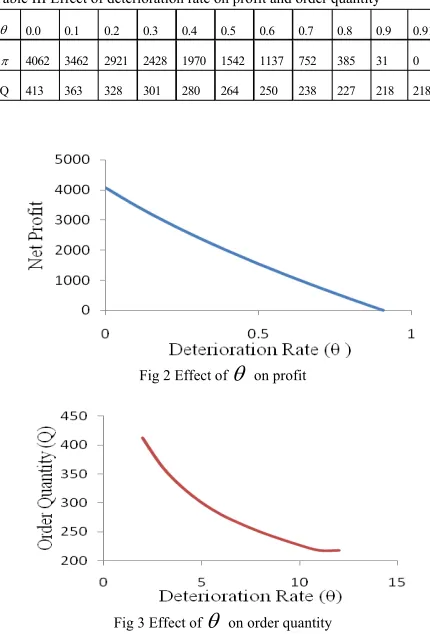
As expected, profit and order size decrease with increasing deterioration rate ( ) as demonstrated by results obtained for Ir =0 and β=0.1 are given in Table III and
[image:4.612.316.531.53.370.2]shown in Fig 2 and Fig 3.
Table III Effect of deterioration rate on profit and order quantity
0.0 0.1 0.2 0.3 0.4 0.5 0.6 0.7 0.8 0.9 0.91
4062 3462 2921 2428 1970 1542 1137 752 385 31 0 Q 413 363 328 301 280 264 250 238 227 218 218
Fig 2 Effect of
on profit [image:4.612.78.294.382.555.2]Fig 3 Effect of
on order quantity
C.Effect of inventory dependent demand factor (β) on profit and order quantity
As demand is dependent on displayed instantaneous inventory level, profit and order quantity are expected to increase with inventory dependent demand factor (β).Model results for input parameters θ=0.1 and Ir =0 are tabulated in Table IV and shown in Fig 4 and Fig 5.It is evident that β has higher impact on profit at its higher values.
Table IV Effect of inventory dependent demand factor (β)on profit and order quantity.
β 0.0 0.1 0.2 0.3 0.4 0.5 0.6 0.7 0.8 0.9 1 1.1 1.2 1.3
3321 3462 3612 3770 3938 4117 4310 4518 4747 5001 5290 5609 6061 6710
Q 390 413 441 474 515 567 634 536 592 666 774 804 1293 2579
[image:4.612.336.512.609.702.2]
Fig 5 Effect of β on order quantity
D.Other Results
1. Both profit and order quantity increase with base demand factor (α), selling price (P). Selling price should be more than Rs.35.77 and purchase cost should be less than Rs.33.86 to earn profit.
2. Profit diminishes as ordering cost increases. Further, order quantity increase with ordering cost and thus conforms square root EOQ formula plus some quantity for deterioration.
V.CONCLUSION
This paper develops order quantity model with non zero cycle ending inventory for continuously deteriorating goods having random shelf life and inventory dependent demand rate. The proposed model is illustrated with numerical example using realistic values from Indian market and impact of deterioration rate, inventory dependent demand factor and reserve inventory at the end of inventory cycle is reported. The results obtained from proposed model conform to the corresponding results for the basic EOQ model when cycle ending inventory is zero, inventory dependent inventory factor and deterioration rate approaches zero. The results indicate that reserve inventory eat into profit and have negative linear relationship with profit. Further, profit is deeply impacted by deterioration rate and followed by inventory dependent demand rate.
This model can be used in determining optimal inventory policy for continuously deteriorating goods such as fruits and vegetables, milk and milk products, bakery products which are mainly sold through supermarket, grocery shops.
REFERENCES
[1] S.K. Goyal and B.C. Giri, “Recent Trends in Modelling of Deteriorating Inventory,” European Journal of Operational Research, vol.134, no.1, pp.1-16, Oct. 2001.
[2] F.Raafat, “Survey of Literature on Continuously Deteriorating Inventory Models,” Journal of the Operational Research Society, vol. 42, no.1, pp. 27-37, Jan.1991.
[3] Wolfe, H. B. “A model for control of style merchandise,” Industrial Management Review, vol.9, no.2, pp69–82, 1968.
[4] R. I. Levin, and C.A. McLaughlin, Productions/Operations Management:
Contemporary Policy for Managing Operating Systems. New York,
McGraw-Hill, 1972.
[5] E. A Silver, and R. Peterson, Decision Systems for Inventory
Management and Production Planning, New York, Wiley, 1985.
[6] R.Gupta and P. Vrat, “Inventory Models for Stock Dependent Consumption Rate,” Opsearch, vol.23, no.1, pp.19-24, Jan.1986.
[7] R.C.Baker and T.Urban, “A Deterministic Inventory System with an Inventory-Level-Dependent Demand Rate,” The Journal of the
Operational Research Society, vol. 39, no.9, pp. 823-831, Sep 1988.
[8] T. K Datta and A.K. Pal, “A note an inventory model with inventory-level dependent rate,” Journal of Operational Research Society, 41(10), 971–975, 1990.1 (1986) 19-24.
[9] G. Padmanabhan and P.Vrat, “EOQ Model for Perishable Items under Stock Dependent Selling Rate,” European Journal of Operational
Research, vol.86, no.2, pp.281-292, Oct.1995.
[10] H.Soni and N.Shah, “Optimal Ordering Policy for Stock-dependent Demand Under Progressive Payment Scheme,” European Journal of
Operational Research, vol.184, no.1, pp.91-100,Jan.2008.
[11] T.Urban, “An Inventory Model with an Inventory-Level-Dependent Demand Rate and Relaxed Terminal Conditions," Journal of the
Operational Research Society, vol.43,no.7, pp.721 – 724, July 1992.
[12] S. Smith and D. Achabal, “Clearance Pricing and Inventory Policies for Retail Chains,” Management Science, vol. 44, no. 3, pp.285-300, Mar.1998.