An Eight Order Two Step Taylor Series Algorithm for the Numerical Solutions of Initial Value Problems of Second Order Ordinary Differential Equations

(1)

ISSN Online: 2333-9721 ISSN Print: 2333-9705

An Eight Order Two-Step Taylor Series

Algorithm for the Numerical Solutions

of Initial Value Problems of Second

Order Ordinary Differential Equations

Ayodele Olakiitan Owolanke

1*

_{, Ohi Uwaheren}

2

_{, Friday Oghenerukevwe Obarhua}

3 1_{Department of Mathematics, Faculty of Mathematical Sciences, Ondo State University of Science and Technology,} Okitipupa, Nigeria

2_{Department of Mathematics, Faculty of Physical Sciences, University of Ilorin, Ilorin, Nigeria} 3_{Mathematical Science Department, Federal University of Technology, Akure, Nigeria}

Abstract

Our focus is the development and implementation of a new two-step hybrid method for the direct solution of general second order ordinary differential equation. Power series is adopted as the basis function in the development of the method and the arising differential system of equations is collocated at all grid and off-grid points. The resulting equation is interpolated at selected points. We then analyzed the resulting scheme for its basic properties. Nu-merical examples were taken to illustrate the efficiency of the method. The results obtained converge closely with the exact solutions.

Subject Areas

Mathematical Analysis

Keywords

Power Series, Collocation and Taylor’s Series Algorithm

1. Introduction

We consider the numerical solution of initial value problem of the form:

(

, ,

) ( )

;

( ) ( )

0 ;

y′′= f x y y′ y a =y y a′ =

γ

(1) In practice, higher order ordinary differential equations of this form

(

1

)

, , , ,

n n

y = f x y y′ ′′ y − , is solved by reducing it to systems of first order

diffe-rential equation of the form:

How to cite this paper: Owolanke, A.O., Uwaheren, O. and Obarhua, F.O. (2017) An Eight Order Two-Step Taylor Series Algori- thm for the Numerical Solutions of Initial Value Problems of Second Order Ordinary Differential Equations. Open Access Lib- rary Journal, 4: e3486.

https://doi.org/10.4236/oalib.1103486

Received: March 2, 2017 Accepted: June 16, 2017 Published: June 19, 2017

This work is licensed under the Creative Commons Attribution International License (CC BY 4.0).

http://creativecommons.org/licenses/by/4.0/

(2)

( ) ( )

, , 0,

[ ]

, , , n

y′ = f x y y a = f ∈c a b x y∈

(2)

then an approximate method is applied to solve the resulting Equation (2) as widely discussed by Fatunla [1] and Lambert [2] and Spiegel [3]. The approach does not utilize additional information associated with the specific ordinary dif-ferential equation, and consequently, the oscillatory nature of the solution of the differential equation is always neglected. Thus, it would be more efficient to im-prove on the numerical method so that higher order ordinary differential equa-tions could be solved without having to reduce to systems of first order as sug-gested by Chakravati and Worland [4], Dahlquist [5], sharp and Fine [6], and Bun and Vasilsyer [7]. Actually, considerable attention has been devoted to solving ordinary differential equation of higher order directly without reduction for instance: methods of linear multistep method (LMM) were considered by Lambert and Watson [8], Dormand and El-Mikkawy [9], El-Mikkawy and El- Desouky [10] and Awoyemi [11][12][13] [14]. Subsequently, LMM was inde-pendently proposed by Kayode [15], Onumanyi et al.[16] and Adesanya et al.

[17] in the predictor-corrector mode, based on collocation method. These au-thors proposed LMM with continuous coefficients where they adopted Taylor series algorithm to supply the starting values. Also, some notable scholars im-prove on the predictor-corrector method for solving ordinary differential equa-tions of higher orders, for instance, Jator and Li [18] proposed five-step and four-step methods respectively in which they adopted a continuous LMM to ob-tain finite difference method. Moreover, Adesanya [19] adopted a method of collocation and interpolation to develop a continuous LMM which is evaluated at different grid points to give discret methods that generate independent solu-tions. Others that adopted block methods include Badmus and Yahaya [20]. One of the advantages of the method is that it provides direct solution of implicit Li-near multistep method without developing separate predictors.

Although some of the aforementioned authors have made use of Taylor series, but little has been said with the use of Taylor series as a major method of im-plementation. So, Our idea is to use Taylor series algorithm to evaluate

, , 1, 2

n j n j

y+ y′+ j= and

1 1 2 3

, , , , , ,

2 3 3 2

n v n v

y+ y′+ v=  and calculate f′, f′′ by the

use partial derivative technique. Thus, two-step hybrid methods in the Taylor se-ries mode are developed to solve second order ordinary differential equations di-rectly.

2. Derivation

In this section, power series is considered as an approximate solution to the general second order problems:

(

, , ,

)

0;

( )

( ) ( )

0 ;

f x y y y′ ′′ = y a =y y a′ =

γ

(3)

of the form:

( )

2 1

0

k j j j

y x a x

+

=

(3)

The first and second derivative of (3) are respectively given as:

( )

2 1 1 1 k j j j

y x ja x

+ − =

′ =

∑

₍₅₎

(

)

2 1 2 2 1 k j j j

y j j a x

+

−

=

′′ =

∑

−

₍₆₎

Combining (2) and (5), we generate the differential system

(

)

(

)

2 1

2

1 , , ,

k

j j j

j j a x f x y y +

−

=

′

− =

∑

(7)

we develop the hybrid scheme using (3) and (5) as interpolation and collocation equations in this work.

Collocating (6) at selected grid and off-grid points, x=xn+1, 0≤ ≤i 2 and

in-terpolating (3) at selected grid and off-grid points, it results into a system of equa-tions:

(

)

2 1

2

1 , 0 2

k

j

j n i

j

j j a x f i

+

− + =

− = ≤ ≤

∑

(8)

2 1

2

, 0 2

k j

j n i

j

a x y i

+

+ =

= ≤ ≤

∑

(9)

where, xn i+ =xn+ih, solving Equations ((7) and (8)), a s′j , yield a method ex-

pressed in the form:

( )

0 0

,

k k

k j n j j n j

j j

y x α x y+ β x f+

= =

=

∑

+

∑

₍₁₀₎

where k=2 and f_n₊_j = f x

(

_n₊_j,y_n₊_j,y_n′₊_j

)

, 0≤2 It implies

2 3 4 5 6 7 8

0 1 n 2 n 3 n 4 n 5 n 6 n 7 n 8 n n

a +a x +a x +a x +a x +a x +a x +a x +a x = y (11)

2 3 4 5 6 7 8

0 1 n1 2 n1 3 n1 4 n1 5 n1 6 n1 7 n1 8 n1 n1

a +a x₊ +a x ₊ +a x₊ +a x₊ +a x₊ +a x₊ +a x ₊ +a x₊ =y₊ (12)

2 3 4 5 6

2 3 4 5 6 7 8

2a +6a xn+12a xn+20a xn +30a xn +42a xn+56a xn = fn

(13)

2 3 4 5 6

2 3 1 4 1 5 1 6 1 7 1 8 1 1

3 3 3 3 3 3 3

2 6 12 20 30 42 56

n n n n n n n

a a x a x a x a x a x a x f

+ + + + + + +

+ + + + + + = (14)

2 3 4 5 6

2 3 2 4 2 5 2 6 2 7 2 8 2 2

3 3 3 3 3 3 3

2 6 12 20 30 42 56

n n n n n n n

a a x a x a x a x a x a x f

+ + + + + + +

+ + + + + + = (15)

2 3 4 5 6

2 3 1 4 1 5 1 6 1 7 1 8 1 1

2a +6a xn+ +12a xn+ +20a xn+ +30a xn+ +42a xn+ +56a xn+ = fn+ (16)

2 3 4 5 6

2 3 4 4 4 5 4 6 4 7 4 8 4 4

3 3 3 3 3 3 3

2 6 12 20 30 42 56

n n n n n n n

a a x a x a x a x a x a x f

+ + + + + + +

+ + + + + + = (17)

2 3 4 5 6

2 3 5 4 5 5 5 6 5 7 5 8 5 5

3 3 3 3 3 3 3

2 6 12 20 30 42 56

n n n n n n n

a a x a x a x a x a x a x f

+ + + + + + +

+ + + + + + = (18)

2 3 4 5 5

2 3 2 4 2 5 2 6 2 7 2 8 2 2

2a +6a x_n₊ +12a x_n₊ +20a x_n₊ +30a x_n₊ +42a x_n₊ +56a x_n₊ = f_n₊ (19)

(4)

2 3 4 5 6 7 8

1 1 1 1 1 1 1 1

2 3 4 5 6

1 3 1 3 1 3 1 3 1 3 1/3

2 3 4 5 6

2 3 2 3 2 3 2 3 2 3 2 3

1 1

0 0 2 6 12 20 30 42 56

0 0 2 6

n n n n n n n n

n n n n n n

n

x x x x x x x x

x x x x x x

x

+ + + + + + + +

+ + + + + +

2 3 4 5 6

1 1 1 1 1 1

2 3 4 5 6

4 3 4 3 4 3 4 3 4 3 4 3

2 3 4 5 6

5 3 5 3 5 3 5 3 5 3 5 3

2 3 4 5 6

2 2 2 2 2 2

12 20 30 42 56

0 0 2 6 12 20 30 42 56

n n n n n

n n n n n n

x x x x x

x x x x x x

+ + + + + + + + + + + + + + + + + + + + + + + +                      0 1 1 2

3 1 3

4 2 3

5 1

6 4 3

7 5 3

8 2 n n n n n n n n n a y a y a f a f a f a f a f a f a f + + + + + + +                           ₌                              (20)

Using Gaussian elimination method, the unknown coefficients a s′j can be

obtained. Putting a s′j back into (3) gives (10):

The coefficients

α

i s′

( )

t ,

β

j s′

( )

t are continuous coefficients obtained using

the transformation

(

1

)

1

n k

t x x

h + −

= − _, t∈

(

0,1

]

d 1

. d

t x=h

Then simplifying the continuous αj s′ , βj s′ , and taking their first derivatives,

we have:

( )

0 1 t h α ′ = − ,

( )

1

t h α ′ = − _,

( )

0 47 13440 h t

β ′ = _,

( )

1 3 327 2240 h t

β ′ = ,

( )

2 3 111 890 h t

β ′ = ,

( )

1 1088 3360 h t

β ′ = _,

( )

4 3 93 640 h t

β ′ = ,

( )

5 3 1095 2240 h t

β ′ = ,

( )

2 1359 13440 h t

β ′ = _.

Then, putting t=1 gives: 2

2 1 2 5 4

3 3

1 2 1

3 3

2 47 810 1377

6720

2252 1377 810 857

n n n n

n n

h

y y y f f f

f f f f

(5)

its first derivative

[

]

2

2 1 2 5 4

3 3

1 2 1

3 3

1

1359 6570 1953

6720

4352 1665 1962 47

n n n n

n n

h

y y y f f f

h

f f f f

+ + + ₊ ₊

+ ₊ ₊



′ = − +  + +





+ + + + _



(22)

with the order

p

=

8

, error constant C₁₀ = −0.0069941, and interval of abso-lute stability X

( ) (

Θ = −14.1608, 0

)

Implementation of the method using Tay-lor series algorithm to evaluate

, , , , ,

n j n j n v n v n v n j

y+ y′+ y+ y′+ f + f + ,

where, j s′ =1, 2 and 1 2 4 5, , , 3 3 3 3

v s′ = and,

(

, ,

)

,

n v n v n v n v

f ₊ = f x₊ y₊ y′₊

such that

( )

2

( )

3

( )

4

2! 3! 4!

n v n n n n n

vh vh vh

y₊ = y +vhy′+ f + f′+ f′′+ (23)

and,

( )

2

( )

3

( )

4

2! 3! 4!

n v n n n n n

vh vh vh

y′₊ =y′+vhf + f′+ f′′+ f′′′+ (24)

Also,

(

)

( )

2

2!

n j n n n n

jh

f ₊ = y′′ x + jh = f + jhf′+ f′′+ (25)

(

, ,

)

n n n n

f = f x y y′

( ) ( )

₍

₎

, , , 1, 2

i i

n n n f = f x y y′ i=

Finding the partial derivative f′ ′′,f , as follows d

d

f f f f

f y f

x x x y

δ δ δ

′ ′

= = + +

′

(26)

(

)

2

d

2 ,

d

f

f Ay Bf Cfy D E

x

′′= = ′+ + ′+ + (27)

where,

2 2

f f

A f

x y y y

∂ ∂

= +

′

∂ ∂ ∂ ∂ (28)

2

f B

x y

∂ =

′

∂ ∂

(29)

f f f

C y f

x y y

∂ _′∂ ∂

= + +

′

∂ ∂ ∂

(30)

( )

2 2 2

2 2

2 2 2

f f f

D y f

x y y

∂ _′ ∂ ∂

= + +

∂ ∂ ∂ ′ (31)

f E f

y ∂ =

(6)

2.1. Analysis of the Properties of the Scheme

We shall consider the analysis of the basic properties of our methods which in-cludes the order, the region of absolute stability and the zero stability of the me-thods.

2.2. Order of Accuracy of the Method

The local truncation error with k-step linear multistep m method which is in line with Lambert (1973), is taken to be linear difference operator  defined by

( )

(

)

(

)

0

;

k

j n j n

j

y x h α y x j hβ y x j =

 

= + − +

 

 

∑

 

 (33)

Thus, expanding (21) as Taylor series about point x and comparing coeffi-cients of k

h , the scheme will be of order

p

=

8

with error constant

2 0.0069941

p

C + = −

( )

, 0

( )

1

( )

2

( )

,

p

n n n p n

L y x h_ _=C y x +C y x′ +C y′′ x + + C y x

(34)

where Cp,p=0,1, are the constant coefficients given as:

(

)

0 0

1 0

1 1

0 0 0

and

1

1 !

k

j j

k

j j

k k k

p p

p j j qj

j j j

C

C j

C j p p j q

p α

α

α β β

=

− −

= = =

  =

  

= _

 

  _{ }

=  − −  + _{ }

  

 

∑

(35)

In line with [2], k-step, linear multistep (21) has order p if

0 1 p1 p

C =C ==C − =C and Cp+1≠0, where, Cp+1≠0 is the error constant.

Subjecting our schemes to equations 35, it is therefore established that linear multistep scheme is of order

p

=

8

, relatively small error constant −0.0069941.

2.3. Consistency of the Scheme

A linear multistep method is consistent if the following conditions are satisfied: 1) The order

p

≥

1

.

2) p

( )

1 =0,p′

( )

1 =

σ

( )

1 .

3) 0 0

k j j= α =

∑

.

4) 0 0

k k

j j

j= jα = j= β

∑

.

2.4. Zero Stability of the Method

Equation (21) has its first characteristic polynomial to be:

( )

2

2 1

r r r

ρ

= − +

₍₃₆₎

The method is zero stable since they have roots r=1 twice.

2.5. Region of Absolute Stability of the Method

(7)

method as in [2]. The method implies that

( )

r

r ρ θ

δ

=

where,

( )

ei cos sin

r= θ =

θ

+i

θ

From scheme (21), we have:

( )

2

2 1

r r r

ρ

= − +

and

( )

1 ₄₇ 2 ₈₁₀ 35 ₁₃₇₇ 43 ₂₂₅₂ ₁₃₇₇ 23 ₈₁₀ 31 ₈₅₇ 6720

r r r r r r r

σ =  + + + + + + 

 

 

so that

( )

e

i

h

θ

ρ

θ

δ

=

which implies

( )

1 ₄₇ 2 ₈₁₀ 35 ₁₃₇₇ 43 ₂₂₅₂ ₁₃₇₇ 23 ₈₁₀ 31 ₈₅₇ 6720

h θ = _ r + r + r + r+ r + r + _

  (37)

( )

cos 2 sin 2 2 cos 2 sin 1

5 5

6720 47 cos 2 47 sin 2 810 cos 810 sin

3 3

4 4

1377 cos 1377 sin 2252 cos 2252 sin

3 3

2 2 2

1377 cos 1377 sin 810 cos 810

3 3 3

h i i

i i

i

θ θ θ θ θ

θ θ

θ θ _θ _θ

θ θ θ

=_ + − − + _

    

× _ + + _ _+ _ _

   



   

+ _ _+ _ _+ +

   

     

+ _ _+ _ _+ _ _+

     

1

2

sin 47

3

i θ

−   _{ +}

  

  

Considering the values of

θ

for 0≤ ≤

θ

180 at intervals of 30θ gives the region of absolute stability to be

(

−14.1608, 0 .

)

3. Numerical Experiments

We test the accuracy of the proposed scheme on some numerical problems, and the results are compared with existing methods.

Problem 1:

( ) ( )

2

( )

0.1

, 0 1, 0 0.5,

32

y′′=x y′ y = y′ = h= (38)

Exact solution

( )

10

1 2

1 log

2 2

x y x

x +

 

= + _ _

−

 

The numerical results of the problem is shown in Table 1, and is compared with Awoyemi and kayode (2005) of order 8 in Table 2.

Problem 2:

(

)

(

( )

2

)

( )

6 4 , 1 1, 1 1, 120

(8)

[image:8.595.207.541.90.193.2]

Table 1. Results and errors for problem (1).

(x) YEX YC ERRNew

0.2 1.100335347731075300 1.100335347731045300 0.00000e 000+

0.4 1.20273255405481600 1.11273255405480200 _{1.010223 10}_× −15

0.6 1.309519604203111900 1.009519604203101000 15

2.886580 10× −

0.8 1.423648930193603500 1.123648930123598200 _{5.029021 10}_× −15

1.0 1.549306144334058600 1.129306144334043400 15

9.169263 10× −

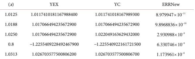
Table 2. Results and errors for problem (2).

(x) YEX YC ERRNew

1.0125 1.0117410181167988400 1.011741018167989300 11

8.979947 10× −

1.0188 1.017066494235672900 1.017066494235672900 _{9.8968836 10}_× −10

1.0250 1.017066494235672900 1.022049163629432000 _{2.930988 10}_× −9

0.8 −1.2255409228492467900 −1.225540922161721500 _{6.330746 10}_× −9

1.0313 1.026703577500806200 1.026703577500806700 _{1.173961 10}_× −8

Note: YEX = Yexact, YC = Ycomputed, ERRNew = Error in new method.

Exact solution

( )

1 ex

y x = −

The numerical results of the problem is shown in Table 2.

4. Conclusion

A Linear Multistep method which implements a Taylor’s series algorithm is de-veloped for the direct solution of general second order initial value problems of ordinary differential equations without reduction to systems of first order diffe-rential equation. The derivatives of continuous scheme to any order were com-puted implementing Taylor’s series algorithm. The accuracy of the method was tested with two test problems, and results were compared with Awoyemi and Kayode [11] of order (8).

References

[1] Fatunla, S.O. (1988) Numerical Methods for Initial Value Problems for Ordinary Differential Equations. Academy Press, New York, 295.

[2] Lambert J.D. (1973) Computational Methods in Ordinary Differential Equations. John Wiley and Sons, New York, 278.

[3] Murray, S.R. (1971) Theory and Problems of Advance Mathematics for Engineers and Scientist. Mc Graw Hill, Inc., New York.

[4] Chakravati, P.C. and Worland, P.B. (1971) A Class of Self Starting Methods for the Numerical Solution of Ordinary Differential Equation. BIT, 11, 368-383.

https://doi.org/10.1007/BF01939405

[5] Dahlquist, G. (1959) Convergence and Stability in the Numerical Integration of Or-dinary Differential Equation. Mathematics Scandinavia, 4, 33-53.

[image:8.595.207.541.224.325.2]

(9)

[6] Sharp and Fine (1992) Some Nystrom Pairs for the General Second Order Value Problem. Journal of Computation and Applied Mathematics, 42, 279-291.

https://doi.org/10.1016/0377-0427(92)90081-8

[7] Bun, R.A. and Vasilsyer, Y.D. (1990) A Numerical Methods for Solving Differential Equations of Any Order. Computational Mathematics and Mathematical Physics, 32, 317-330.

[8] Lambert, J.D. and Wastson, A. (1976) Symmetric Multistep Method for Periodic In-itial Value Problem. Journal of the Institute of Mathematics Application, 18, 189- 202. https://doi.org/10.1093/imamat/18.2.189

[9] Dormand, J.R., El-Mikkawy, M.E.A. and Prince, P.J. (2003) Families of Runge Kutta Nystrom Formula, IMA. Journal of Numerical Analysis, 7, 235-250.

https://doi.org/10.1093/imanum/7.2.235

[10] El-Mikkawy, M.E. and El-Desouky, R. (2003) A New Optimized Non FSAL Em-bedded Runge-Kutta-Nystrom Algorithms of Order 6 and 4 in Six Stages. Applied Mathematics and Computation, 145, 33-43.

https://doi.org/10.1016/S0096-3003(02)00436-8

[11] Awoyemi, D.O. and Kayode, S.J. (2005) A Maxima Order Collocation Method for Initial Value Problems of General Second Order Ordinary Differential Equation. Proceeding of the Conference Organized by the National Mathematical Center, Ab-uja.

[12] Awoyemi, D.O. (1999) A Class of Continuous Method for General Second Order Initial Value Problems in Ordinary Differential Equations. International Journal of Computer Mathematics, 72, 29-37.https://doi.org/10.1080/00207169908804832 [13] Awoyemi, D.O. (2001) A New Sixth Order Algorithms for General Second Order

Ordinary Differential Equation. International Journal of Computer Mathematics, 77, 117-124.https://doi.org/10.1080/00207160108805054

[14] Awoyemi, D.O. (2005) An Algorithm Collocation Methods for Direct Solution of Special and General Fourth Order Initial Value Problems of Ordinary Differential Equation. Journal of Nigerian Association of Mathematical Physics, 6, 271-238. [15] Kayode, S.J. (2009) An Order Zero Stable Method for Direct Solution of Fourth

Order Ordinary Differential Equation. American Journal of Applied Sciences, 5, 1461-1466.

[16] Onumanyi, P., Sirisons, U.W. and Dauda, Y. (2001) Toward Uniformly Accurate Continuous Finite Difference Approximation of Ordinary Differential Equation.

Bayero Journal of Pure and Applied Sciences, 1, 5-8.

[17] Adesanya, A.O., Anake, T.A. and Udoh, M.O. (2008) Improved Continuous Me-thod for Direct Solution of General Second Order Ordinary Differential Equation.

Journal of Nigeria Association of Mathematical Physics, 13, 59-62.

[18] Jator, S.N. and Li, J. (2009) A Self Stationary Linear Multistep Method for a Direct Solution of General Second Order Initial Value Problem. International Journal of Computer Mathematics, 86, 817-1165.

[19] Adesanya, A.O. (2011) Block Methods for Direct Solution of General Higher Order Initial Value Problem of Ordinary Differential Equations. PhD Thesis, Federal Uni-versity of Technology, Akure.

[20] Badmus, A.M. and Yahaya, Y.A. (2009) An Accurate Uniform Order 6 Block Me-thod for Direct Solution of General Second Order Ordinary Differential Equations.

(10)

Submit or recommend next manuscript to OALib Journal and we will pro-vide best service for you:

 Publication frequency: Monthly

 ₉_{subject areas}_{of science, technology and medicine}

 _{Fair and rigorous peer-review system}  Fast publication process

 _{Article promotion in various social networking sites (LinkedIn, Facebook, Twitter,} etc.)

 _{Maximum dissemination of your research work}

Submit Your Paper Online: Click Here to Submit