2017, Volume 4, e3593 ISSN Online: 2333-9721 ISSN Print: 2333-9705
3D Matrix Ring with a “Common” Multiplication
Orgest Zaka
Department of Mathematics, Faculty of Technical Science, University of Vlora “Ismail QEMALI”, Vlora, Albania
Abstract
In this article, starting from geometrical considerations, he was born with the idea of 3D matrices, which have developed in this article. A problem here was the definition of multiplication, which we have given in analogy with the usual 2D matrices. The goal here is 3D matrices to be a generalization of 2D ma-trices. Work initially we started with 3 3 3× × matrix, and then we extended
to m n× ×p matrices. In this article, we give the meaning of 3D matrices. We also defined two actions in this set. As a result, in this article, we have reached to present 3-dimensional unitary ring matrices with elements from a field F.
Subject Areas
Algebra, Applied Statistical Mathematics, Geometry
Keywords
Linear Algebra, Matrices, Ring Theory
1. Introduction
Based on the meaning of the addition and the multiplication of 2D matrices [1]-[6], this article stretches this sense, the idea, the addition and the multiplica-tion of 3D matrices. Starting from geometrical consideramultiplica-tions, concretely taking into account the cube, he was born with the idea of 3D matrices, which have de-veloped in this article. A problem here was the definition of multiplication, for which we have acted pages, analogously acted as the columns, which we have given in analogy with the usual 2D matrices [6][9]. The goal here is 3D matrices to be a generalization of 2D matrices. We proved that this set of two actions to-gether in forming the “unitary ring” [7][8][10][11]. In literature and in various mathematical forums, we noticed an interest in the 3D matrices, but on the other hand are missing results associated with them; this was a sufficient reason to explore. We introduced the meaning of the scalar multiplication, and finally How to cite this paper: Zaka, O. (2017) 3D
Matrix Ring with a “Common” Multipli- cation. Open Access Library Journal, 4: e3593.
https://doi.org/10.4236/oalib.1103593
Received: April 11, 2017 Accepted: May 12, 2017 Published: May 15, 2017
Copyright © 2017 by author and Open Access Library Inc.
This work is licensed under the Creative Commons Attribution International License (CC BY 4.0).
http://creativecommons.org/licenses/by/4.0/
we have shown that we have an F-module connected to this ring 3D matrices or vector spaces [8][10]. As indications for this paper were simply geometric im-aginations. Everything presented in this article are my results.
2. Addition of 3 × 3 × 3, 3-D Matrices over Field
F
, and the
Addition Abelian Group of Their 3-D Matrices
Imagining a parallelepiped, with born idea of 3D matrices, which are define as follows
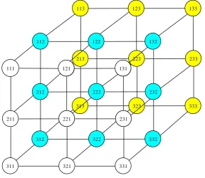
Definition 2.1 3-dimensional 3 × 3 × 3 matrice will call, a matrix which has:
three horizontal layers (analogous to three rows), three vertical page (analogue
with three columns in the usual matrices) and three vertical layers two of which are hidden.
The set of these matrices the write how:
( )
{
( )
}
3 3 3× × F = aijk |aijk∈F and i=1, 2, 3;j=1, 2, 3;k=1, 2, 3
The appearance of these matrices will be as in Figure 1.
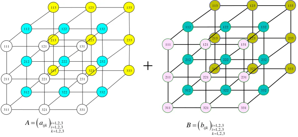
Definition 2.2 The addition of two matrices A3 3 3× × ,B3 3 3× × ∈3 3 3× ×
( )
F we will call the matrix:( )
{
}
{
}
3 3 3× × = cijk |cijk =aijk+bijk,∀i j k, , ∈ 1, 2, 3
C
The appearance of the addition of 3 × 3 × 3, 3D matrices, will be as in Figure 2, where matrices A and B have the following appearance,
( )
{
}
( )
{
}
3 3 3
3 3 3
| for 1, 2, 3; 1, 2, 3; 1, 2, 3
| for 1, 2, 3; 1, 2, 3; 1, 2, 3
ijk ijk ijk ijk
a a F i j k
b b F i j k
× × × ×
= ∈ = = =
= ∈ = = =
A
B
111
231 221
211
131 121
331 321
311
112
232 222
212
132 122
332 322
312
113
233 223
213
133 123
333 323
313 121
221 231
[image:2.595.229.518.469.719.2]131
111
231 221
211
131 121
331 321
311 112
232 222
212
132 122
332 322
312
113
233 223
213
133 123
333 323
313 121
221 231
131 111
231 221
211
131 121
331 321
311 112
232 222
212
132 122
332 322
312
113
233 223
213
133 123
333 323
313 121
221 231 131
( )
1,2,3 1,2,3 1,2,3i ijk i k
A
a
= = ==
( )
1,2,31,2,3 1,2,3
i ijk i k
B
b
= = ==
[image:3.595.58.536.73.293.2]+
Figure 2. The addition of 3 × 3 × 3, 3D matrices.
Definition 2.3 Zero matrix 3 × 3, 3D we will called the matrix that has all its elements zero.
( )
{
}
3 3 3× × = 0F ijk|i=1, 2, 3;j=1, 2, 3;k=1, 2, 3
O
Definition 2.4. The opposite matric of anmatrice
( )
{
}
3 3 3× × = aijk |i=1, 2, 3;j=1, 2, 3;k=1, 2, 3
A
will, called matrix
( )
{
}
3 3 3× × aijk |i 1, 2, 3;j 1, 2, 3;k 1, 2, 3
−A = − = = =
(where −aijk is a opposite element of element aijk∈F, so aijk+ −
( )
aijk =0Fand
(
F, ,+ ⋅)
is field [8][10][11]), which satisfies the condition(
)
{
(
(
)
)
}
( )
{
}
3 3 3 3 3 3
3 3 3
| 1, 2, 3; 1, 2, 3; 1, 2, 3
0 | 1, 2, 3; 1, 2, 3; 1, 2, 3
ijk ijk
ijk
a a i j k
i j k
× × × ×
× ×
+ − = + − = = =
= = = = =
A A
O
Theorem 2.1
(
3 3 3× ×( )
F ,+)
is a beliangrup.Proof: Truly from the definition 2.2, of addition the 3-Dmatrices, we see that
addition is the sustainable in 3 3 3× ×
( )
F , because{
}
, , , , 1, 2, 3
ijk ijk ijk ijk ijk
a ∈F b ∈ ⇒F c =a +b ∈F ∀i j k∈
1) Associative property,
( )
aijk ,( )
bijk ,( )
cijk 3 3 3× ×( ) (
F)
(
)
∀ =A B= C= ∈
⇒ A+B + = +C A B+C truly(
)
( ) ( ) ( ) (
) ( ) (
(
)
)
(
)
(
(
)
)
( ) (
)
(
)
ijk ijk ijk ijk ijk ijk ijk ijk ijk ijk ijk ijk ijk ijk ijk ijk ijk ijk
a b c a b c a b c
a b c a b c a b c
+ + = + + = + + = + +
= + + = + + = + + = + +
A B C
2) ∀ =A
( )
aijk ∈
3 3 3× ×( )
F ,∃ =O( )
0ijk /A O+ = + =O A A.truly, ∀ =A
( )
aijk ∈
3 3 3× ×( )
F ,∃ =O( )
0ijk /A O+ = + =O A A.( )
( )
{
}
(
)
{
}
( )
{
}
0 | 1, 2, 3; 1, 2, 3; 1, 2, 3
0 | 1, 2, 3; 1, 2, 3; 1, 2, 3
| 1, 2, 3; 1, 2, 3; 1, 2, 3
ijk ijk
ijk ijk
ijk
a i j k
a i j k
a i j k
+ = + = = =
= + = = =
= = = = =
A O
A
3) ∀ =A
( )
aijk ∈
3 3 3× ×( )
F ,∃ − = −A( )
aijk ∈
3 3 3× ×( )
F /A+ −( )
A =O. truly, from Definition 2.4, we have( )
{
(
(
)
)
}
( )
{
}
| 1, 2, 3; 1, 2, 3; 1, 2, 3
0 | 1, 2, 3; 1, 2, 3; 1, 2, 3
ijk ijk
ijk
a a i j k
i j k
+ − = + − = = =
= = = = =
A A
O
4) Addition is commutative.
( )
aijk ,( )
bijk 3 3 3× ×( )
F , . ∀ =A B= ∈
A+ = +B B Atruly
( ) ( ) (
)
( , ) is abelian(
) ( ) ( )
ijk ijk ijk ijk ijk ijk ijk ijk
a b a b b a b a
+
+ = + = + = + = + = +
A B B A
3. Addition of
m n
× ×
p
, 3-D Matrices over Any Field
F
and
the Addition Abelian Group of Their 3-D Matrices
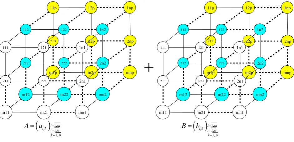
Definition 3.1 3-dimensionalmxnxp matrix will call, a matrix which has: m-
horizontal layers (analogous to m-rows), n-vertical page (analogue with n-col-
umns in the usualmatrices) and p-vertical layers (p − 1 of which are hidden). The set of these matrixes the write how:
( )
{
( )
| -field and 1, ; 1, ; 1,}
m n p× × F = aijk aijk∈F i= m j= n k= p
Definition 3.2 The addition of two matrices A B, ∈m n p× ×
( )
F we will call the matrix:( )
{
| , 1, ; 1, ; 1,}
m n p× × = cijk cijk =aijk+bijk ∀ =i m j= n k= p
C
The appearance of the addition of mxnxp, 3D matrices will be as in Figure 3, where matrices A and B have the following appearance,
( )
{
}
( )
{
}
| 1, ; 1, ; 1,
| 1, ; 1, ; 1,
m n p ijk m n p ijk
a i m j n k p
b i m j n k p
× × × ×
= = = =
= = = =
A
B
Definition 3.3 3-D, Zero matrix m n× ×p, we will called the matrix that has all its elements zero.
( )
{
0 | 1, ; 1, ; 1,}
m n p× × ijk i m j n k p
= = = = =
O O
Definition 3.4 The opposite matric of anmatrice
( )
{
| 1, ; 1, ; 1,}
( )
m n p× × = aijk i= m j= n k= p ∈ m n p× × F
A
111
231 221
211
131 121
mn1 m21
m11 112
2n2 222
212
1n2 122
mn2 m22
m12
11p
2np 22p
213
1np 12p
mnp m2p
m1p 121
221 2n1 1n1
( )
1, 1, 1,i m ijk i n k p
A
a
= = ==
+
111
231 221
211
131 121
mn1 m21
m11 112
2n2 222
212
1n2 122
mn2 m22
m12
11p
2np 22p
213
1np 12p
mnp m2p
m1p 121
221 2n1 1n1
( )
1, 1, 1,i m ijk i n k p
B
b
= = = [image:5.595.62.533.71.298.2]=
Figure 3. The addition of mxnxp, 3D matrices.
( )
{
| 1, ; 1, ; 1,}
( )
m n p× × aijk i m j n k p m n p× × F
−A = − = = = ∈
(where −aijk is a opposite element of element aijk∈F, so aijk+ −
( )
aijk =0Fand
(
F, ,+ ⋅)
is field), which satisfies the condition(
)
{
(
(
)
)
}
( )
{
}
| 1, ; 1, ; 1,
0 | 1, ; 1, ; 1,
m n p m n p ijk ijk
ijk
a a i m j n k p
i m j n k p
× × + − × × = + − = = =
= = = = =
A A
O
Theorem 3.1
(
m n p× ×( )
F ,+)
is abeliangrup.Proof: Truly from the definition 3.2, of additions the 3-D matrices, we see that
addition is the sustainable inm n p× ×
( )
F , because, , 1, ; 1, ; 1,
ijk ijk ijk ijk ijk
a ∈F b ∈ ⇒F c =a +b ∈F ∀ =i m j= n k= p
1) Associative property,
( )
aijk ,( )
bijk ,( )
cijk m n p× ×( ) (
F)
(
)
∀ =A B= C= ∈
⇒ A+B + = +C A B+C truly(
)
( ) ( ) ( ) (
) ( ) (
(
)
)
(
)
(
(
)
)
( ) (
)
(
)
ijk ijk ijk ijk ijk ijk ijk ijk ijk ijk ijk ijk ijk ijk ijk ijk ijk ijk
a b c a b c a b c
a b c a b c a b c
+ + = + + = + + = + +
= + + = + + = + + = + +
A B C
A B C
2) ∀ =A
( )
aijk ∈
m n p× ×( )
F ,∃ =O( )
0ijk ∈
m n p× ×( )
F /A O+ = + =O A A.truly,
( )
aijk m n p× ×( )
F ,( )
0ijk m n p× ×( )
F / .∀ =A ∈
∃ =O ∈
A O+ = + =O A A( )
( )
{
}
(
)
{
}
( )
{
}
0 | 1, ; 1, ; 1,
0 | 1, ; 1, ; 1,
| 1, ; 1, ; 1,
ijk ijk
ijk F ijk
ijk
a i m j n k p
a i m j n k p
a i m j n k p
+ = + = = =
= + = = =
= = = = =
A O
3) ∀ =A
( )
aijk ∈
m n p× ×( )
F ,∃ − = −A( )
aijk ∈
m n p× ×( )
F /A+ −( )
A =O.truly, from Definition 2.4, we have
( )
{
(
(
)
)
}
( )
{
}
| 1, ; 1, ; 1,
0 | 1, ; 1, ; 1,
ijk ijk
F ijk
a a i m j n k p
i m j n k p
+ − = + − = = =
= = = = =
A A
O
4) Addition is commutative.
( )
aijk ,( )
bijk m n p× ×( )
F / .∀ =A B= ∈
A+ = +B B Atruly
( ) ( ) (
)
(F, ) is abelian(
) ( ) ( )
ijk ijk ijk ijk ijk ijk ijk ijk
a b a b b a b a
+
+ = + = + = + = + = +
A B B A
4. The “Common” Multiplication of
3 3 3
× ×
, 3-D Matrices
with Elements Froman Field
F
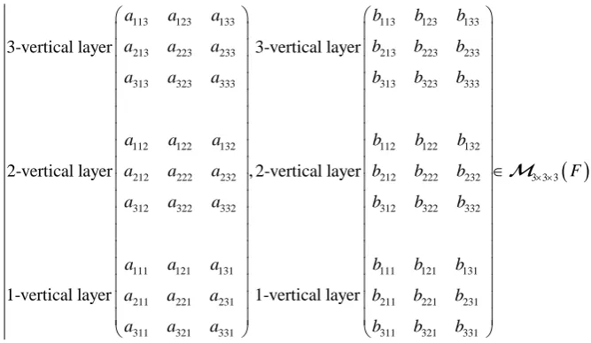
Definition 4.1: The multiplication of two matrices A B, ∈3 3 3× ×
( )
F we willcall the matrix C= ⊗ ∈A B 3 3 3× ×
( )
F calculated as follows:113 123 133
213 223 233
313 323 333
112 122 132
212 222 232
312 322 332
111 121 131
211 221 231
311 321 331
3-vertical layer
3-2-vertical layer
1-vertical layer
,
a a a
a a a
a a a
a a a
a a a
a a a
a a a
a a a
a a a
∀
113 123 133
213 223 233
313 323 333
112 122 132
212 222 232 3 3
312 322 332
111 121 131
211 221 231
311 321 331
vertical layer
2-vertical layer
1-vertical layer
b b b
b b b
b b b
b b b
b b b
b b b
b b b
b b b
b b b
× × ∈
3
( )
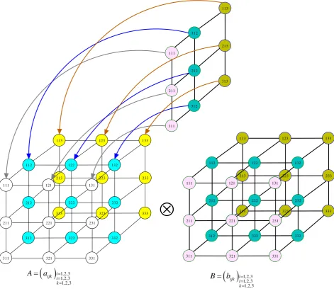
F [image:6.595.203.537.317.511.2]The appearance of the multiplication of 3 × 3 × 3, 3D matrices will be as in
Figure 4.
(
)
(
)
(
)
113 123 133 113
213 223 233
313 323 333
112 122 132
212 222 232
312 322 332
111 121 131
211 221 231
311 321 331
3-vertical layer
2-vertical layer
1-vertical layer
c c c a a
c c c
c c c
c c c
c c c
c c c
c c c
c c c
c c c
= = C
123 133 113 123 133
213 223 233 213 223 233
313 323 333 313 323 333
112 122 132 112 122 132
212 222 232 212 222 232
312 322 332
111 121 131
211 221 231
311 321 331
a b b b
a a a b b b
a a a b b b
a a a b b b
a a a b b b
a a a
a a a
a a a
a a a
⊗
312 322 332
111 121 131
211 221 231
311 321 331
b b b
b b b
b b b
b b b
111
231 221
211
131 121
331 321
311 112
232 222
212
132 122
332 322
312
113
233 223
213
133 123
333 323
313 121
221 231
131 111
231 221
211
131 121
331 321
311 112
232 222
212
132 122
332 322
312
113
233 223
213
133 123
333 323
313 121
221 231 131
( )
1,2,3 1,2,3 1,2,3i ijk i k
A
a
= = ==
( )
1,2,31,2,3 1,2,3
i ijk i k
B
b
= = ==
⊗
111
211
311 112
212
312
113
213
[image:7.595.60.532.76.494.2]313
Figure 4. The multiplication of 3 × 3 × 3, 3D matrices.
111 111 111 121 211 131 311
112 112 112 122 211 132 312
113 113 113 123 213 133 313
;
;
;
c a b a b a b
c a b a b a b
c a b a b a b
= ⋅ + ⋅ + ⋅
= ⋅ + ⋅ + ⋅
= ⋅ + ⋅ + ⋅
211 211 111 221 211 231 311
212 212 112 222 211 232 312
213 213 113 223 213 233 313
;
;
;
c a b a b a b
c a b a b a b
c a b a b a b
= ⋅ + ⋅ + ⋅
= ⋅ + ⋅ + ⋅
= ⋅ + ⋅ + ⋅
311 311 111 321 211 331 311
312 312 112 322 211 332 312
313 313 113 323 213 333 313
;
;
;
c a b a b a b
c a b a b a b
c a b a b a b
= ⋅ + ⋅ + ⋅
= ⋅ + ⋅ + ⋅
= ⋅ + ⋅ + ⋅
the second vertical page is:
121 111 121 121 221 131 321
122 112 122 122 222 132 322
123 113 123 123 223 133 323
;
;
;
c a b a b a b
c a b a b a b
c a b a b a b
= ⋅ + ⋅ + ⋅
= ⋅ + ⋅ + ⋅
221 211 121 221 221 231 321
222 212 122 222 222 232 322
223 213 123 223 223 233 323
;
;
;
c a b a b a b
c a b a b a b
c a b a b a b
= ⋅ + ⋅ + ⋅
= ⋅ + ⋅ + ⋅
= ⋅ + ⋅ + ⋅
321 311 121 321 221 331 321
322 312 122 322 222 332 322
323 313 123 323 223 333 323
;
;
;
c a b a b a b
c a b a b a b
c a b a b a b
= ⋅ + ⋅ + ⋅
= ⋅ + ⋅ + ⋅
= ⋅ + ⋅ + ⋅
and third vertical page is:
131 111 131 121 231 131 331
132 112 132 122 232 132 332
133 113 133 123 233 133 333
;
;
;
c a b a b a b
c a b a b a b
c a b a b a b
= ⋅ + ⋅ + ⋅
= ⋅ + ⋅ + ⋅
= ⋅ + ⋅ + ⋅
231 211 121 221 221 231 321
232 212 122 222 222 232 322
233 213 123 223 223 233 323
;
;
;
c a b a b a b
c a b a b a b
c a b a b a b
= ⋅ + ⋅ + ⋅
= ⋅ + ⋅ + ⋅
= ⋅ + ⋅ + ⋅
331 311 121 321 221 331 321
332 312 122 322 222 332 322
333 313 123 323 223 333 323
;
;
;
c a b a b a b
c a b a b a b
c a b a b a b
= ⋅ + ⋅ + ⋅
= ⋅ + ⋅ + ⋅
= ⋅ + ⋅ + ⋅
It is reduce the above notes through matrix blocks
3 3 3 3 3
2 2 2 2 2
1 1 1 1 1
×
= ⊗ = ×
×
C A B A B
C A B A B
C A B A B
where
111 121 131 112 122 132 113 123 133
1 211 221 231 2 212 222 232 3 213 223 233
311 321 331 312 322 332 313 323 333
111 121 131
1 211 221 231
311 321 331
; ; ;
;
a a a a a a a a a
a a a a a a a a a
a a a a a a a a a
b b b
b b b
b b b
= = =
=
A A A
B
112 122 132 113 123 133
2 212 222 232 3 213 223 233
312 322 332 313 323 333
; ;
b b b b b b
b b b b b b
b b b b b b
= =
B B
3 3 3 3 3
2 2 2 2 2
1 1 1 1 1
×
= ⊗ = ×
×
C A B A B
C A B A B
C A B A B
and
111 121 131 112 122 132 113 123 133
1 211 221 231 2 212 222 232 3 213 223 233
311 321 331 312 322 332 313 323 333
; ;
c c c c c c c c c
c c c c c c c c c
c c c c c c c c c
= = =
C C C
1= 1× 1; 2 = 2× 2; 3 = 3× 3
C A B C A B C A B
Remark 4.1 Two dimensional matrices can think like matrix with size
1
m n× ×
Easy seen from the definition 1, above it that, if aij2=0,aij3=0 and 2 0, 3 0,
ij ij
b = b = ∀i j, ∈
(
1, 2, 3)
we get, the usual 3 × 3-matrix multiplication,would say that: A2=0; A3=0; B2=0; B3=0):
111 111 121 211 131 311 111 121 121 221 131 321 111 131 121 231 131 331
211 111 221 211 231 311 211 121 221 221 231 321 211 121 221 221 231 321
311 111 321 211 331
a b a b a b a b a b a b a b a b a b
a b a b a b a b a b a b a b a b a b
a b a b a b
⋅ + ⋅ + ⋅ ⋅ + ⋅ + ⋅ ⋅ + ⋅ + ⋅
⋅ + ⋅ + ⋅ ⋅ + ⋅ + ⋅ ⋅ + ⋅ + ⋅
⋅ + ⋅ + ⋅ 311 a311 b121 a321 b221 a331 b321 a311 b121 a321 b221 a331 b321
⋅ + ⋅ + ⋅ ⋅ + ⋅ + ⋅
Definition 4.2. The3-D,unit matrix, associated with the “common” multipli-cation, must be:
3 3 3
1 0 0
0 1 0 t vertical layer
vertical layer
t hi
he first vertic rd
0 0 1
1 0 0
0 1 0 the second
0 0 1
1 0 0
0 1 0
0 0
al layer
1
× ×
=
I
or, in the language of matrix blocks:
3 3
3 3 3 3 3
3 3
×
× × ×
×
=
I
I I
I
Easy distinguish that, ∀ ∈A 3 3 3× ×
( )
F /A⊗I3 3 3× × =A.Theorem 4.1
(
3 3 3× ×( )
F ,⊗)
is a unitary semi-Group with regard to this ordinary multiplicationProof: 1) associative property. ∀A B C, , ∈3 3 3× ×
( )
F(
)
(
)
(
)
( )
( )
(
)
(
)
(
)
3 3
3 3 3 3 3 3 3 3 3
2 2 2 2 2 2 2 2 2
1 1 1 1 1 1 1 1 1
3 3 3 3
, is a semigroup
2 2 2 2
1 1 1
F
A B C
A B C
A B C
× ×
× × ×
⊗ ⊗ = × ⊗ = × ×
× × ×
× ×
= × × =
× ×
A B C A B C
A B C A B C
A B C A B C
A B C A
A B C A
A B C
3 3
2 2
1 1 1
.
⊗ ⊗
B C
B C
A B C
2) ∃I3 3 3× × ∈3 3 3× ×
( )
F /∀ ∈A 3 3 3× ×( )
F ⇒ ×A I3 3 3× × = A.( )
( 3 3 )
3 3 3 3 3 3 , is a unitary semigroup 3
2 3 3 2 3 3 2
1 3 3 1 3 3 1 F
×
× × ×
× ×
× ×
×
⊗ = × =
×
A I A I A
A I A I A
A I A I A
Theorem 4.2
(
3 3 3× ×( )
F , ,+ ⊗)
is a unitary Ring.Proof: 1) From Theorem 2.1.
(
3 3 3× ×( )
F ,+)
is abeliangrup.2) From Theorem 4.1.
(
3 3 3× ×( )
F ,⊗)
is a unitary semi-Group, and conse-quently also,(
3 3 3× ×( )
F ,⊗)
is a unitary semi-Group3) ∀A B C, , ∈3 3 3× ×
( )
F ,(
)
(
)
truly
(
)
(
(
)
)
(
)
( )
( 3 3 )
3 3 3 3 3 3 3 3 3
2 2 2 2 2 2 2 2 2
1 1 1 1 1 1 1 1 1
3 3 3 3
, , is a unitary Ring
2 2 2 2
1 1
F
× + ×
+ × +
⊗ + = ⊗ + = ⊗ + = × + + × +
× + ×
= × + ×
× +
A B C A B C A B C
A B C A B C A B C A B C
A B C A B C A B C
A B A C
A B A C
A B A
3 3 3 3
2 2 2 2
1 1 1 1 1 1
3 3 3 3
2 2 2 2
1 1 1 1
.
× ×
= × + ×
× × ×
= ⊗ + ⊗ = ⊗ + ⊗
A B A C
A B A C
C A B A C
A B A C
A B A C A B A C
A B A C
In a similar manner proved the point (b).
5. Multiplication of a 3-D,
3 3 3
× ×
-Matrix by a Scalar
Definition 5.1 The multiplication of matrix A∈3 3 3× ×
( )
F with scalar Fλ ∈ , is matrix C=λA∈3 3 3× ×
( )
F :113 123 133 113 123 133
213 223 233 213 223 233
313 323 333 313 323
112 122 132
212 222 232
312 322 332
111 121 131
211 221 231
311 321 331
a a a a a a
a a a a a a
a a a a a a
a a a
a a a
a a a
a a a
a a a
a a a
λ λ λ
λ λ λ
λ λ λ
λ
⋅ ⋅ ⋅
⋅ ⋅ ⋅
⋅ ⋅ ⋅
= =
C
333
112 122 132
212 222 232
312 322 332
111 121 131
211 221 231
311 321 331
a a a
a a a
a a a
a a a
a a a
a a a
λ λ λ
λ λ λ
λ λ λ
λ λ λ
λ λ λ
λ λ λ
⋅ ⋅ ⋅
⋅ ⋅ ⋅
⋅ ⋅ ⋅
⋅ ⋅ ⋅
⋅ ⋅ ⋅
⋅ ⋅ ⋅
So
( )
( )
(
)
3 3 3 3 3 3
:
,
F F F
λ
λ
× × × ×
× →
A A
Theorem 5.1
(
3 3 3× ×( )
F , ,+ F)
is a vector spaceProof. is evident because,
(
3 3×( )
F , ,+ F)
it is the vector space, see [6][8][9][10].
Definition 5.2 The multiplication of matrix A∈m n p× ×
( )
F with scalar Fλ ∈ , is matrix C=λA∈m n p× ×
( )
F :wherein each element of the matrix is multiplied (by multiplication of the field
F) with the element λ ∈F. Well, so we have
( )
(
)
: ( )
,
m n p m n p
F F F
λ λ
× × × ×
× →
A A
Theorem 5.2
(
m n p× ×( )
F , ,+ F)
is a vector spaceProof. Is evident because,
(
m n×( )
F , ,+ F)
it is the vector space, see [6][8]6. Conclusion
In this article, based on geometric considerations, and mostly considering the cube, we managed to develop the idea of the 3D matrix doing so a generalization of the 2D matrices, step by step. Furthermore, we gave a unitary ring with the elements of a field F. Initially we gave the ring 3 3 3× × , 3D matrices and then
generalized this concept for m n× ×p, 3D matrices. At the end of this article, we present the scalar multiplication with the 3D matrices and we show that the set of 3 3 3× × , 3D matrix, forms a vector space over the field F.
References
[1] Artin, M. (1991) Algebra. Prentice Hall, Upper Saddle River.
[2] Bretscher, O. (2005) Linear Algebra with Applications. 3rd Edition, Prentice Hall, Upper Saddle River.
[3] Connell, E.H. (2004) Elements of Abstract and Linear Algebra.
[4] Schneide, H. and Barker, G.P. (1973) Matrices and Linear Algebra (Dover Books on Mathematics). 2nd Revised Edition.
[5] Lang, S. (1987) Linear Algebra. Springer-Verlag, Berlin, New York.
[6] Nering, E.D. (1970) Linear Algebra and Matrix Theory. 2nd Edition, Wiley, New York.
[7] Zaka, O. and Filipi, K. (2016) The Transform of a Line of Desargues Affine Plane in an Additive Group of Its Points. International Journal of Current Research, 8, 34983-34990.
[8] Zaka, O. (2013) Abstract Algebra II. Vllamasi, Tirana. [9] Zaka, O. (2013) Linear Algebra I. Vllamasi, Tirana. [10] Zaka, O. (2013) Linear Algebra II. Vllamasi, Tirana.
[11] Zaka, O. and Filipi, K. (2016) One Construction of an Affine Plane over a Corps. Journal of Advances in Mathematics, 12.
Submit or recommend next manuscript to OALib Journal and we will pro-vide best service for you:
Publication frequency: Monthly
9 subject areas of science, technology and medicine Fair and rigorous peer-review system
Fast publication process
Article promotion in various social networking sites (LinkedIn, Facebook, Twitter, etc.)
Maximum dissemination of your research work
Submit Your Paper Online: Click Here to Submit