On the predictive power of implied volatility indexes: A comparative analysis with GARCH forecasted volatility

Munich Personal RePEc Archive

On the predictive power of implied

volatility indexes: A comparative analysis

with GARCH forecasted volatility

Bentes, Sonia R and Menezes, Rui

24 October 2012

Online at

https://mpra.ub.uni-muenchen.de/42193/

On the predictive power of implied volatility indexes: A comparative analysis with GARCH forecasted volatility

Sonia R. Bentes1* and Rui Menezes2

¹ISCAL, Av. Miguel Bombarda, 20, 1069-035, Lisbon, Portugal ²ISCTE, Av. das Forças Armadas, 1649-025, Lisbon, Portugal

Abstract

This paper examines the behavior of several implied volatility indexes in order to

compare them with the volatility forecasts obtained from estimating a GARCH model.

Though volatility has always been a prevailing subject of research it has become

particularly relevant given the increasingly complexity and uncertainty of stock

markets in these days. An important measure to assess the market expectations of the

future volatility of the underlying asset is the implied volatility (IV) indexes.

Generally, these indexes are calculated based on the prices of out-of-the money put

and call options on the underlying asset. Sometimes called the “investor fear gauge”,

the IV indexes are a measure of the implied volatility of the underlying index. This

study focuses on the implied and GARCH forecasted volatility of some emerging

countries and some developed countries. More specifically, it compares the predictive

power of the IV indexes with the ones provided by standard volatility models such as

the ARCH/GARCH (Autoregressive Conditional Heteroskedasticity Model/

Generalized Autoregressive Conditional Heteroskedasticity Model) type models.

Finally, a debate of the results is also provided.

Keywords: implied volatility; volatility forecasts, GARCH models, volatility indices

* Corresponding author.

Introduction

Volatility has always been central to financial theory. A number of reasons have been

advanced for that. While Martens and van Dick (2007) considers that assessing

financial volatility is important for portfolio management, risk management and

option pricing, Daly (2008) identifies, in a more extensive way, six reasons for this

interest: (i) first, sharp asset prices fluctuations may lead to an erosion of confidence

in the stock markets and reduced flow of capital into this equity markets; (ii)

secondly, it is an important factor to determine the probability of bankruptcy of

individual firms; (iii) thirdly, it is crucial to determine the bid-ask spread and the

market liquidity; (iv) hedging techniques are affected by the volatility level since the

price of insurance increases with volatility; (v) high volatility may reduce the level of

participation in the economic activity with negative consequences to the investment;

and, (vi) Finally, increased volatility may induce regulatory agencies to force firms to

allocate a larger percentage of capital to cash equivalent investment to the potential

detriment of efficiency in allocations. For a more comprehensive debate on the

subject see also Bollerslev et al. (1992), Figlewski (1997) and Poon and Granger

(2003).

Given the increasing turbulence and instability of stock markets, volatility has become

a very active field of research. An important issue in this debate is how well implied

volatility (IV) predicts future realized volatility (RV). The former is based on the

theory of options by solving the BS model in order to determine the (corresponding)

implied volatility, denoted by  . Sometimes called the “the investor fear gauge”

(Whaley, 2000), IV is widely regarded as the options market’s forecast of future

volatility. Thus, if option markets are efficient, market implied volatility should be an

efficient forecast of future returns volatility. In other words, IV should include the

information contained in all the variables in the market information set (Christensen

and Prabhala, 1998). Thought several studies have addressed this subject no definite

answer has come out as empirical results have been mixed so far. In the light of this,

the purpose of our paper is to examine the predictive power of IV, compare it to the

volatility derived from a GARCH-type model and check which one is more suitable to

Besides the need for a re-assessment of the predictive power of IV our research is

motivated by another shortcoming in the literature: generally, studies on this topic are

mainly devoted to developed economies, with only very few focusing only on

emerging countries. In fact, there is a variety of studies concerning the IV of futures,

individual assets, stock market indexes, oil and some other commodities traded in

developed economies such as US and EU (Blair, 2001, Becker, 2006, Chen, 2007,

Szakmary et al. 2003, inter alia) but very little regarding implied volatility in

emerging markets (e.g., Nam et al., 2006; Vrugt, 2009). This may be due to the fact

that only recently IVs started to be available in some of these countries (see, for

example, India, Korea).

Early papers (e.g. Latane and Rendleman, 1976, Chiras and Manaster, 1978 and

Beckers, 1981) found that implied volatilities are better estimates of future volatility

than the traditional standard deviation. In a subsequent research, Jorion (1995)

documents that IV is an efficient, though biased, predictor of future volatility for

foreign currency futures. In the same line, Fleming et al. (1995) for future markets

indexes, Christensen and Prabhala (1998) for SP 100 index options and Giot (2003)

came to similar results. Subsequently, Szakmary et al. (2003) using data from 35

future option markets concluded that for a large majority of the commodities studied

the implieds outperform the historical volatility as a predictor of RV. Further, GARCH

forecasts are not superior to IVs. A slightly different conclusion arise Agnolucci

(2009) who studied the predictive power of IV and GARCH models. According to this

author while IV does not perform better than GARCH models, there is some

information contained in IV forecasts that is not contained in those obtained from the

GARCH-type models.

In contrast with this stream of research where IV dominates, Day and Lewis (1992),

and Lamoureux and Lastrapes (1993), for SP 100 and options on ten stocks,

respectively, found that implied volatility is biased and inefficient since past

volatilities contains predictive information about future volatility beyond that

provided by implieds. This is in consonance with Kumar and Shastri (1990),

Randolph et al. (1990) and Canina and Fliglewsi (1993) who generally concluded that

IV has little power to predict RV. More specifically, the latter found that there is no

Prabhala (1998), Canina and Figlewski (1993) findings may be due to a shorter time

horizon used in their study, which exactly precedes the October 1987 crash, where a

regime shift occurred. Therefore, implied volatility is expected to be more biased

before the crash than afterwards. Apart from this cause, some other reasons may

explain this kind of results (Agnolucci, 2009): (i) sample selection bias, given the

difficulty in observing IV during periods of high turbulence where stock market

liquidity becomes a problem to investors (Engle and Rosenberg, 2000); (ii) sample

bias, which occurs when IV takes into account the presence of low probability events

which are not too common in the sample. (iii) bid-ask spreads and, finally, (iv) the use

of BS model to get the IV of American options. On the other end, critics of IV argue

consider the latter is not a good predictor of future realized volatility since market

prices are determined by several other factors, which are not included in the BS

formula, such as, market liquidity and the BS assumption of unlimited arbitrage.

Given this controversy further researches seem to be needed. This is specially so as

very few studies address the IV predictive power of emerging economies. In sum, our

paper makes at least three contributions to literature: (i) it updates early researches on

IV; (ii) it focuses on emerging economies and (iii) it applies an alternative approach,

based on ADL and ECM, to assess the information content of implieds in explaining

realized volatility, which to the best of out knowledge has not yet been done so far.

More specifically, the latter model adds by clearly separating the short and long run

effects in explaining the relation between implied and realized volatility.

The remainder of the paper is organized as follows: Section 2 describes the

methodological background. Section 3 presents the empirical results and, finally, in

Section 4 we draw the conclusions.

2. Metodological background

In this section we discuss the theoretical framework that motivates the empirical

analysis. According to the conventional approach the information content of implied

volatility is typically assessed by an OLS regression of the form:

0

t i t t

where RVt denotes the realized volatility for the period t and IVt represents the implied

volatility at the beginning of period t. From expression (1) three hypotheses can be

tested. First (H1) if IV contains at least some information about future realized

volatility, coefficient _i should be nonzero. Second (H2) if IV is an unbiased estimate

of realized volatility then ₀ 0 and _i 1. Finally (H3) if implied volatility is

efficient, the residuals u_t should be white noise, non-auto correlated, and uncorrelated

with any other variable.

Subsequently, to compare the efficiency of implied volatility to that of past realized

volatility a multiple regression of the form is estimated:

0 1

t i t h t t

RV   IV  RV_ u . (2)

Thus (H4) if iIVt is an efficient forecast, h should be not statistically significant

and the values of the R2 and the information criteria of Eq. (2) should be not

significantly different from those of Eq. (1).

Though some literature exists which applies this methodology very few studies cover

the emerging countries. Additionally, we contribute to the existing literature by

introducing an Autoregressive Distributed Lag – ADL(p,q) Model and an Error

Correction Model – ECM to study the above-mentioned relationships, which to the

best of our knowledge has not been done so far.

An ADL (p,q) model is of the form

0 _{0 1} ,

q p

t _k ik t k _j hj t j t

RV  





and is used to assess dynamical relations between the variables. This is useful for our

purposes since it encompasses not only the contemporaneous relations, where a

change in one or more explanatory variables causes instant changes in the dependent

variable, but also lagged relations between the variables.













p

t _k k t k ih t p i t p t

RV _  IV_  RV_  IV_ 

 



where





adjustment speed, that is, how RV changes in response to disequilibrium. In the

context of univariate modeling taking the first differences to get stationarity seems to

be acceptable. However, when the relationship between variables is relevant such a

procedure is inappropriate. This is especially so because first difference models only

capture short run relations, neglecting the long-run effects. To overcome this problem

a solution is to estimate an ECM where both relations are accounted for. Also

denominated Equilibrium Correction Model it is interpreted as follows: RV changes

between t and t1 as a result of 1) changes in the explanatory variable IV between t

and t1 and 2) to correct for any disequilibrium during the previous period.

Alternatively, a GARCH framework can be used to compute the estimated volatility

and compare the results with IVs. This is in line with the work of Engle (1992) who

considers that financial market volatility may be predictable. Bearing on this he

derived the ARCH(q) model. Consider the time series RV_t and the associated

prediction error _t RV_tE RV_{t1 t} where E_t1 is the expectations operator

conditioned on time t1 information. By definition, _t is serially uncorrelated with

mean zero but the conditional variance of the process 2

t

 is changing over time. In the

classic ARCH(q) process proposed by Engle (1982) _t2 is postulated to be a linear

function of the lagged squared innovations implying Markovian dependence dating

back only q periods; that is, _{t i}2_ for i1, 2,...,q. That is:

 

2 2

t L t

     (5)

A Generalized Autoregressive Conditional Heteroskedasticity (GARCH) was then

defined by Bollerslev (1986) so that _t z_t_t, z_t is i.i.d., with zero mean and unit

variance

 

 

2 2 2

,

t L t L t

where 0, 

 

 





order q and p, respectively. For stability and covariance stationarity of the _t

process, all the roots of _1

 

 

 

outside the unit circle.

3. Empirical results

3.1 Data and sampling procedure

To conduct our analysis we gathered data from several different countries, such as:

BRIC (Brazil, Russia, India and China), some Australasian economies (Korea,

Hong-Kong and Australia) and the US, which are used as a benchmark. The choice of these

particular spot indexes had to do with the availability of data of the corresponding

implied volatility indexes, which are not published for all the emerging countries in

the world. This has limited our study to the above-mentioned markets. Thus, the spot

indexes used are: BOVESPA (Brazil), RTS Standard Index (Russia), S&P CNX

NIFTY (India), CSI 300 (China), KOSPI (Korea), Hang-Seng (Hong-Kong),

S&P/ASX (Australia) and SPX (US). The correspondingly IVs indexes comprise:

VBOV (Brasil), RTSVX (Russia), INVIXN (India), IVCSI (China), KIX (Korea),

VHSI (Hong-Kong), AVIX (Australia) and VIX (US), respectively.

Since IVs of each market are not available for the same period and in order not to

waste any information contained in the data, which may be crucial to understand the

volatility phenomenon, different time lengths were considered for each IV. The reason

for this lies in the fact that IVs started to be traded in very different moments in time

according to each Board of Exchange. This is not critical as the aim of our study is to

compare the predictive power of IV with RV and GARCH forecasts within each

country and not amongst countries. Therefore, our empirical analysis is based on the

following time spans: Brazil – Oct 2003 to July 2012; Russia – Feb 2006 to July

2012; India – Dec 2007 to July 2012; China – Feb 2005 to July 2012; Korea and

Hong Kong – Oct 2003 to July 2012; Australia – Feb 2008 to July 2012 and US – Oct

2003 to July 2012. For the same reason, the different calculating methods of IVs do

on the BS formula. In brief, it represents the expected volatility of the underlying

index (SP 100) over the next 30 days. It was calculated by inverting the BS formula in

order to determine _t. In September 2003 the method of calculation of VIX changed.

There are mainly two differences between the old and the new VIX: (i) first, it is

based on the SP 500, which is considered a benchmark for the US market; and, (ii)

second it is model free, which constitutes its major advantage over the former.

Notwithstanding these changes, some emerging countries still rely on the old method.

Another issue which arises when analyzing stock market volatility refers to the

method of measuring it. This occurs because volatility is a latent variable. As a result

a proxy needs to be computed so that comparisons may be performed (Agnolucci,

2009). Following the established practice in literature (e.g., Christensen and Prabhala,

1998) monthly realized volatility is utilized in our study as a proxy:

2 22

1 1

260

100 ln

22

t i i t i

P RV

P

   

  

  _{  }

 

 



To determine the 30 days realized volatility non-overlapping observations were used.

Data was collected from the Bloomberg database.

3.2 Descriptive statistics

The descriptive statistics for the realized, implied and GARCH volatility for each

Table 1

Descriptive statistics of realized volatilities

Brazil Russia India China Korea Hong-Kong Australia US

Mean 26.66169 32.34871 25.65043 27.93043 22.04173 22.42545 19.93018 17.15169 Median 24.40421 25.47996 20.52604 23.93731 19.15381 17.99045 18.36917 13.59675 Maximum 110.3256 144.1859 79.00021 60.21619 85.31131 109.4227 59.98454 82.27708 Minimum 13.28732 12.19904 10.05383 11.46747 9.797445 7.141296 8.629115 6.493272 Std. Dev. 13.22811 21.84182 14.08291 11.70870 11.13861 14.45839 9.694242 12.29182 Skewness 3.272464 2.869206 1.778287 0.911113 2.750250 2.848526 2.000438 2.687427 Kurtosis 18.68150 13.05460 6.238763 2.925273 13.80391 14.94017 8.361718 12.00547

Jarque-Bera 1275.293 435.5790 53.99054 12.47286 649.1618 773.0224 100.6988 485.7782 Probability 0.000000 0.000000 0.000000 0.001957 0.000000 0.000000 0.000000 0.000000

Observations 106 78 56 90 106 106 54 106

Table 2

Descriptive statistics of implied volatilities

Brazil Russia India China Korea Hong-Kong Australia US

Mean 47.21525 40.78711 29.18929 39.16783 24.62170 25.49745 25.45017 20.89925 Median 51.86696 32.83595 25.90500 44.93935 22.70500 21.46000 24.23500 17.79000 Maximum 72.59250 167.8919 69.32000 68.05720 81.27000 79.95000 54.12580 59.89000 Minimum 16.01067 18.85370 16.56000 7.753600 14.68000 11.72000 14.56530 10.42000 Std. Dev. 16.95852 25.41428 10.64901 20.10892 9.360423 11.75645 8.614555 9.558026 Skewness -0.262687 3.199907 1.459176 -0.318112 3.011471 1.775554 1.220109 1.744656 Kurtosis 1.641992 15.03222 5.464257 1.616900 15.89406 6.880860 4.224089 6.399371 Jarque-Bera 9.364230 603.6286 34.04180 8.691549 894.5192 122.2155 16.76937 104.8120 Probability 0.009259 0.000000 0.000000 0.012961 0.000000 0.000000 0.000228 0.000000

Observations 106 78 56 90 106 106 54 106

Table 3

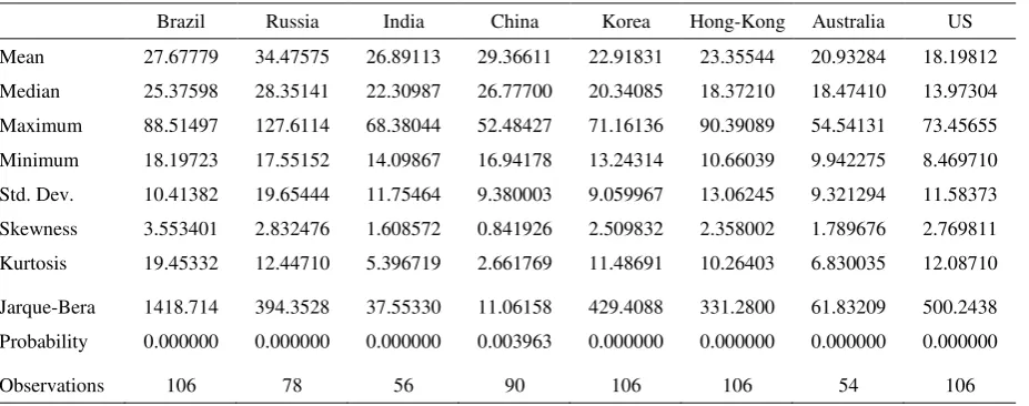
Descriptive statistics of the GARCH forecasted volatilities

Brazil Russia India China Korea Hong-Kong Australia US Mean 27.67779 34.47575 26.89113 29.36611 22.91831 23.35544 20.93284 18.19812 Median 25.37598 28.35141 22.30987 26.77700 20.34085 18.37210 18.47410 13.97304 Maximum 88.51497 127.6114 68.38044 52.48427 71.16136 90.39089 54.54131 73.45655 Minimum 18.19723 17.55152 14.09867 16.94178 13.24314 10.66039 9.942275 8.469710 Std. Dev. 10.41382 19.65444 11.75464 9.380003 9.059967 13.06245 9.321294 11.58373 Skewness 3.553401 2.832476 1.608572 0.841926 2.509832 2.358002 1.789676 2.769811 Kurtosis 19.45332 12.44710 5.396719 2.661769 11.48691 10.26403 6.830035 12.08710

Jarque-Bera 1418.714 394.3528 37.55330 11.06158 429.4088 331.2800 61.83209 500.2438 Probability 0.000000 0.000000 0.000000 0.003963 0.000000 0.000000 0.000000 0.000000

As we are dealing with different time horizons, the number of observations for each

index varies. Thus, while Brazil, Korea, Hong-Kong and the US total 106

observations, Russia adds up to 78, India to 56, China to 90 and Australia to 54.

Starting with the mean average we find that implied volatilities exceed the

corresponding realized volatility for all the time series considered. This finds support

in Corrado and Miller (2003) and Christensen and Prabhala (1998), where similar

results were documented. Furthermore, the mean difference between realized and

implied volatility is substantially greater for Brazil, China and Russia whereas Hong

Kong, US and Korea present the shortest differences. Regarding the standard

deviation, results are somewhat mixed: India, Korea, Hong-Kong, Australia and US

implied volatility show lower dispersion than the realized ones. The opposite holds

for the remainder countries. When we take into consideration the GARCH estimates a

similar pattern to the realized volatility arises for the mean and standard deviation.

In addition, all the three proxies considered generally show positive skewness

(exception made for VBOV and IVCSI) and excess kurtosis. This statistic is only

lower than 3 for China realized and implied volatilities and the GARCH volatility

estimates and for Brazil implied volatility, which may suggest that these countries

might have distinct volatility behaviour when compared to the remainder ones. As

expected all volatility series show significant departures from normality as indicated

by the Jarque Bera test and may exhibit fat tails since most of them are leptokurtic.

Figures A1-A8 (Appendix A) provide a graphical analysis of the implied, realized and

GARCH volatilities for each country. Apart from Brazil and China, whose descriptive

statistics have already denoted a distinct behaviour, some common patterns seem to

arise: (i) volatility series appear to be synchronized since realized volatility in month

m is aligned with implied in the last trading day of month m1. The same occurs

with GARCH volatilities. Differences that might occur in this pattern may be due to

forecasting errors. (ii) Generally, a consistent behaviour is found for all the proxies

considered. (iii) Moreover, RV and GARCH volatilities are closer to each other than

the IVs, which might suggest that GARCH volatility is apparently a better predictor of

the realized ones than the IV. (iv) Implied volatilities do not anticipate RVs when

3.3 Results

3.3.1 Implied Volatility

Table 4 presents the estimates of ₀ and _i (Eq. 1) for the four emergent markets

(Brazil, Russia, India and China), and for Korea, Hong-Kong, Australia and US.

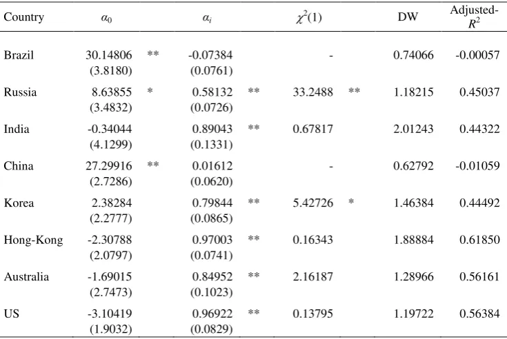
Table 4

OLS Implied volatility estimates (Eq. 1)

Country α0 αi 2

(1) DW

Adjusted-R2

Brazil 30.14806 ** -0.07384 - 0.74066 -0.00057

(3.8180) (0.0761)

Russia 8.63855 * 0.58132 ** 33.2488 ** 1.18215 0.45037 (3.4832) (0.0726)

India -0.34044 0.89043 ** 0.67817 2.01243 0.44322

(4.1299) (0.1331)

China 27.29916 ** 0.01612 - 0.62792 -0.01059

(2.7286) (0.0620)

Korea 2.38284 0.79844 ** 5.42726 * 1.46384 0.44492

(2.2777) (0.0865)

Hong-Kong -2.30788 0.97003 ** 0.16343 1.88884 0.61850 (2.0797) (0.0741)

Australia -1.69015 0.84952 ** 2.16187 1.28966 0.56161 (2.7473) (0.1023)

US -3.10419 0.96922 ** 0.13795 1.19722 0.56384

(1.9032) (0.0829)

Standard error estimates are in brackets ** Statistically significant at the 1% level * Statistically significant at the 5% level

The results above show that, for the BRIC countries, the constant term 0 is

non-significantly different from zero except for India. For the same subset, the slope

coefficient _i only appears significantly in the regressions for Russia (0.58132) and

India (0.89043). A 2(1) test for the null hypothesis that _i 1 was also performed and the null was not only rejected for India. Thus, for the BRIC countries, H1 (IV

contains at least some information about future RV) is only statistically confirmed for

Russia and India. On the other hand, H2 (IV is an unbiased estimate of the future RV),

does not appear to contain any information that can be useful to predict future RV, at

least in the long-run equilibrium relationship.

Turning now to the estimates of ₀ and _i (Eq. 1) for Korea, Hong-Kong, Australia

and the US, Table 4 show that the null hypothesis of ₀ 0 is not rejected in every

case, whereas _i 0 is rejected at 1% or lower in all cases. Furthermore, the 2(1)

test for the null hypothesis of _i 1 is only rejected (at the 5% level) for Korea, thus

supporting the conclusion that IV contains at least some information about future RV

(H1) in all these cases, and that IV is an unbiased estimate of the future RV (H2) in

Hong-Kong (αi=0.97003), Australia (αi=0.84952) and the US (αi=0.969).

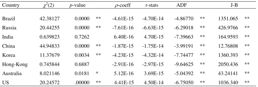
Finally, regarding H3 (IV is efficient if the residuals ut are white noise, non-auto

correlated and uncorrelated with any other variable). Table 5 presents the residual’s

diagnostics of autocorrelation [Breusch-Godfrey serial correlation LM test - 2(2)] and Pearson correlation with the explanatory variable for each regression. ADF tests

on the residuals rejected the null of a unit root in all cases. Likewise, tests for

residual’s normality also rejected the null for all countries. Therefore, apart from stationarity and the evidence of no correlation of the residuals with other variables, H3

is not (globally) confirmed in any of the estimated regressions.

Table 5

OLS Implied volatility residual’s diagnostics (Eq. 1)

Country 2(2) p-value -coeff t-stats ADF J-B

Brazil 42.38127 0.0000 ** -4.61E-15 -4.70E-14 -4.86770 ** 1351.065 ** Russia 20.44255 0.0000 ** -7.61E-16 -6.63E-15 -6.29018 ** 426.9766 ** India 0.639823 0.7262 6.40E-16 4.70E-15 -7.39663 ** 164.9593 ** China 44.94833 0.0000 ** -1.87E-15 -1.75E-14 -3.99191 ** 12.76808 ** Korea 11.37679 0.0034 ** -4.23E-15 -4.32E-14 -7.74477 ** 1360.393 ** Hong-Kong 0.745844 0.6887 -2.91E-16 -2.97E-15 -9.64625 ** 2050.436 ** Australia 8.021146 0.0181 * 5.12E-16 3.69E-15 -5.04392 ** 43.24141 ** US 20.24572 .00000 ** 4.41E-15 4.50E-14 -6.75050 ** 1036.340 ** ** Statistically significant at the 1% level

Table 6 exhibits the estimates of ₀, _i and _h (Eq. 2) for the countries considered

in this study.

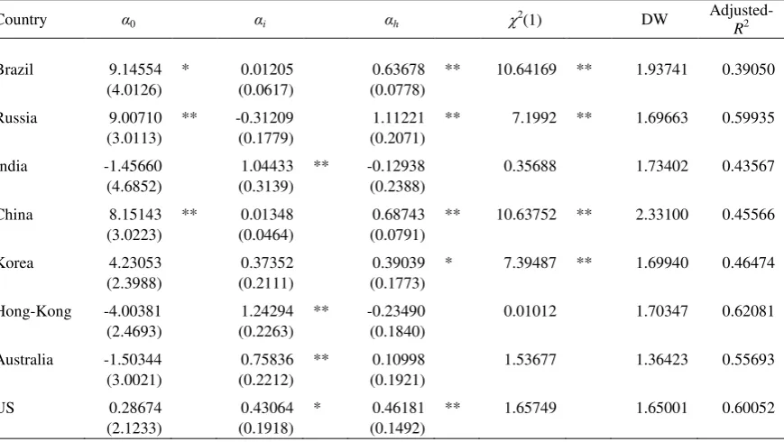
Table 6

AR(1) Implied volatility estimates (Eq. 2)

Country α0 αi αh 2_{(1) DW}

Adjusted-R2

Brazil 9.14554 * 0.01205 0.63678 ** 10.64169 ** 1.93741 0.39050

(4.0126) (0.0617) (0.0778)

Russia 9.00710 ** -0.31209 1.11221 ** 7.1992 ** 1.69663 0.59935

(3.0113) (0.1779) (0.2071)

India -1.45660 1.04433 ** -0.12938 0.35688 1.73402 0.43567

(4.6852) (0.3139) (0.2388)

China 8.15143 ** 0.01348 0.68743 ** 10.63752 ** 2.33100 0.45566

(3.0223) (0.0464) (0.0791)

Korea 4.23053 0.37352 0.39039 * 7.39487 ** 1.69940 0.46474

(2.3988) (0.2111) (0.1773)

Hong-Kong -4.00381 1.24294 ** -0.23490 0.01012 1.70347 0.62081

(2.4693) (0.2263) (0.1840)

Australia -1.50344 0.75836 ** 0.10998 1.53677 1.36423 0.55693

(3.0021) (0.2212) (0.1921)

US 0.28674 0.43064 * 0.46181 ** 1.65749 1.65001 0.60052

(2.1233) (0.1918) (0.1492)

Standard error estimates are in brackets ** Statistically significant at the 1% level * Statistically significant at the 5% level

The hypothesis to be tested in this regression consists in comparing the efficiency of

the IV to that of the past RV, with the null _h 0. This only holds for India,

Hong-Kong and Australia. For these countries we also found out that the R2 coefficients are

not significantly different between both regressions (India: 0.44322 vs. 0.43567;

Hong-Kong: 0.61850 vs. 0.62081; Australia: 0.56161 vs. 0.55693). Similarly,

Schwarz Information Criterion provided the same conclusions (India: 7.64961 vs.

7.73650; Hong-Kong: 7.28572 vs. 7.32426; Australia: 6.66631 vs. 6.74229). A 2(1) test for the null hypothesis that  _i _h 1 was performed and the null was not

rejected for India, Hong-Kong and Australia.

Although the residuals of the estimated regressions are stationary for all countries

(ADF tests were performed and the null hypothesis of a unit root was rejected at the

1% level or lower, in all cases), it is worthy to note that the residual’s serial

RV in Eq. (1) and additionally, to some extent, in Eq. (2). This is evidenced by the low

DW statistics obtained in all cases except for India (2.01243) in Eq. (1) and, to some

extent, for Hong-Kong (1.88884). Nevertheless, the AR(1) results obtained from

estimating Eq. (2), for these two countries, did not improve the DW statistic, on the

contrary they turned out to be worse. In the attempt to avoid this problem we

estimated eight ADL(p,q) models for the same financial markets analyzed before.

This was conducted by estimating Eq. (3), where the number of lags on RV (p) and IV

(q) were chosen in order to eliminate the residual’s autocorrelation. For our purpose, p

= q≤ 2 was enough to eliminate the autocorrelation (the number of lags used in each

case differ from country to country). A summary of the results is presented in Table 7.

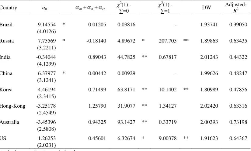
Table 7

ADL(p,q) [p≤ 2 and q≤ 2] Implied volatility estimates (Eq. 3)

Country α0 i0i1i2

2

(1) -

∑=0 

2

(1) -

∑=1 DW Adjusted-R2

Brazil 9.14554 * 0.01205 0.03816 - 1.93741 0.39050

(4.0126)

Russia 7.75569 * -0.18140 4.89672 * 207.705 ** 1.89863 0.63435 (3.2211)

India -0.34044 0.89043 44.7825 ** 0.67817 2.01243 0.44322

(4.1299)

China 6.37977 * 0.00442 0.00929 - 1.99626 0.48247

(3.1241)

Korea 4.46194 0.71499 63.8171 ** 10.1402 ** 1.80989 0.47856 (2.3415)

Hong-Kong -3.25178 1.25790 31.9077 ** 1.34127 2.02420 0.63316 (2.4549)

Australia -3.45396 0.94325 93.1427 ** 0.33719 2.00393 0.73198 (2.5808)

US 1.26253 0.45601 6.32674 * 9.00378 ** 1.91623 0.64367

(2.0231)

Standard error estimates are in brackets ** Statistically significant at the 1% level * Statistically significant at the 5% level

To verify H1 in this model, we should test whether i0 iq 0. A 

2

(1) test for

the null hypothesis of _i0 _iq 0 (q = 0, , 2) was performed. The null was

not only rejected for Brazil and China. To verify H2, 0 0 and i0 iq 1 (q =

Hong-Kong and Australia however the null _i0 _iq 1 was rejected at less than 1%

for the US.

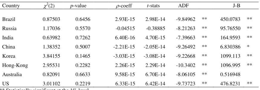
Finally, H3 can be verified by looking at the properties of the residuals ut (Table 8).

Serial correlation, correlation with the explanatory variable and stationarity are no

longer a problem. However, normality is not only rejected for Australia. Despite this

limited evidence, we believe that ADL regressions provide a better framework for the

type of analysis under consideration than static OLS regressions.

Table 8

ADL(p,q) [p≤ 2 and q≤ 2] Implied volatility residual’s diagnostics (Eq. 3)

Country 2_{(2) p-value }_{-coeff t-stats ADF J-B}

Brazil 0.87503 0.6456 2.93E-15 2.98E-14 -9.84962 ** 450.0783 ** Russia 1.17036 0.5570 -0.04515 -0.38885 -8.21263 ** 95.76550 ** India 0.63982 0.7262 6.40E-16 4.70E-15 -7.39663 ** 164.9593 ** China 1.38352 0.5007 -2.21E-15 -2.05E-14 -9.26492 ** 6.830386 * Korea 3.84155 0.1465 -3.03E-15 -3.08E-14 -9.22668 ** 1099.113 ** Hong-Kong 2.95531 0.2282 2.26E-15 2.29E-14 -10.3402 ** 1096.995 ** Australia 0.82091 0.6633 9.58E-15 6.70E-14 -8.06105 ** 0.516948

US 3.01102 0.2219 6.33E-15 6.42E-14 -9.73723 ** 476.8231 **

** Statistically significant at the 1% level * Statistically significant at the 5% level

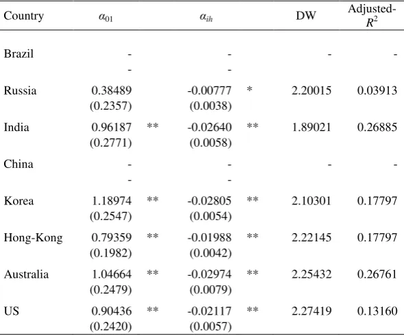
On the basis of the ADL(1,1) model one can obtain the corresponding ECM for the

countries with significant _i in the static OLS regression. This leads us to the

exclusion of Brazil and China from this analysis. Table 9 shows the ECM implied

volatility estimates ₀₁ and _ih for all the other countries. The ₀₁ coefficient

provides information about the short-run adjustment of RV on IV while _ih indicates

Table 9

ECM Implied volatility estimates (Eq. 4)

Country α01 αih DW

Adjusted-R2

Brazil - - - -

- -

Russia 0.38489 -0.00777 * 2.20015 0.03913

(0.2357) (0.0038)

India 0.96187 ** -0.02640 ** 1.89021 0.26885 (0.2771) (0.0058)

China - - - -

- -

Korea 1.18974 ** -0.02805 ** 2.10301 0.17797 (0.2547) (0.0054)

Hong-Kong 0.79359 ** -0.01988 ** 2.22145 0.17797 (0.1982) (0.0042)

Australia 1.04664 ** -0.02974 ** 2.25432 0.26761 (0.2479) (0.0079)

US 0.90436 ** -0.02117 ** 2.27419 0.13160

(0.2420) (0.0057)

Standard error estimates are in brackets ** Statistically significant at the 1% level * Statistically significant at the 5% level

As can be seen, there are both significant short- and long-run adjustments in the

relationship between IV and RV for India, Korea, Hong-Kong, Australia and US. For

Russia there are only significant long-run adjustments. The short-run coefficients span

from 0.79 to 1.19, whereas the speed of adjustment coefficient ranges from 0.01 to

0.03. This means that a deviation from the long-run relationship between RV and IV

takes a very short time to re-attain equilibrium, with the lowest duration occurring for

Russia.

3.3.2 GARCH Forecasted Volatility

This subsection focus on the results obtained from regressing the realized volatility

(RV) on the GARCH forecasted volatility (GV). Table 10 presents the estimates of ₀'

and _i' (Eq. 1) for all the countries under consideration. The models used in these

computations are those defined in Section 2, Eq. (2-4). To compute these estimates

volatility was obtained by the model _t2   

 

 

estimates the monthly time series was constructed by

22 2

1

260 100

22 i t

GV 



 



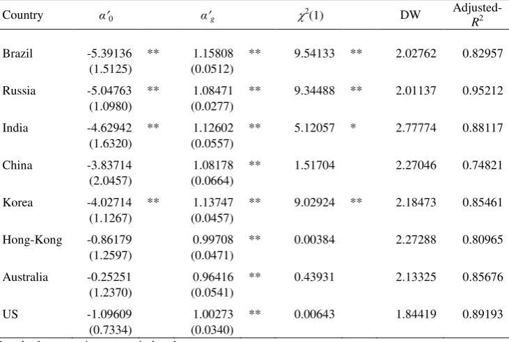
Table 10

OLS GARCH volatility estimates (Eq. 1)

Country α0 αg 2(1) DW

Adjusted-R2

Brazil -5.39136 ** 1.15808 ** 9.54133 ** 2.02762 0.82957 (1.5125) (0.0512)

Russia -5.04763 ** 1.08471 ** 9.34488 ** 2.01137 0.95212 (1.0980) (0.0277)

India -4.62942 ** 1.12602 ** 5.12057 * 2.77774 0.88117 (1.6320) (0.0557)

China -3.83714 1.08178 ** 1.51704 2.27046 0.74821

(2.0457) (0.0664)

Korea -4.02714 ** 1.13747 ** 9.02924 ** 2.18473 0.85461 (1.1267) (0.0457)

Hong-Kong -0.86179 0.99708 ** 0.00384 2.27288 0.80965 (1.2597) (0.0471)

Australia -0.25251 0.96416 ** 0.43931 2.13325 0.85676 (1.2370) (0.0541)

US -1.09609 1.00273 ** 0.00643 1.84419 0.89193

(0.7334) (0.0340)

Standard error estimates are in brackets ** Statistically significant at the 1% level * Statistically significant at the 5% level

It is worthy to note that the constant term estimates α0 are significantly different from

zero (1%) in the regressions for Brazil, Russia, India and Korea, while the slope

coefficient estimates αi are significantly non-zero (1%) in all regressions. For the null

'

1

i

  , the 2(1) test denotes non-rejection for China, Hong-Kong, Australia and the

US, and rejection at 5% for India. Thus, H1 is confirmed in all cases and H2 is

confirmed for China, Hong-Kong, Australia and the US. Although these results do not

depart much from those obtained by implied volatility (IV), the overall performance

of the models is greatly improved, as can be seen by the R2 coefficients obtained.

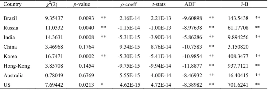
Regarding H3, Table 11 presents the residual’s diagnostics as described above. There

serial correlation is still present in the regressions for Brazil, Russia, India, Korea and

US.

Table 11

OLS GARCH volatility residual’s diagnostics (Eq. 1)

Country 2(2) p-value -coeff t-stats ADF J-B

Brazil 9.35437 0.0093 ** 2.16E-14 2.21E-13 -9.60898 ** 143.5438 ** Russia 11.0332 0.0040 ** -1.15E-14 -1.00E-13 -8.97638 ** 61.17708 ** India 14.3631 0.0008 ** -5.31E-15 -3.90E-14 -5.86286 ** 9.894256 ** China 3.46968 0.1764 9.34E-15 8.76E-14 -10.7583 ** 3.150820 Korea 16.7471 0.0002 ** -5.30E-15 -5.41E-14 -10.9854 ** 408.3477 ** Hong-Kong 3.85708 0.1454 -9.75E-15 -9.94E-14 -11.8877 ** 937.7121 ** Australia 0.78049 0.6769 5.55E-15 4.00E-14 -8.46932 ** 16.40415 ** US 7.69442 0.0213 * 4.62E-15 4.72E-14 -8.38982 ** 701.6241 ** ** Statistically significant at the 1% level

* Statistically significant at the 5% level

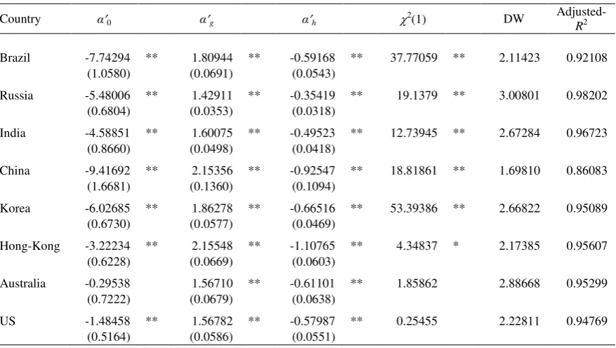
Table 12 presents the estimates of ₀', _g' and _h' (Eq. 2) for every country. The null

hypothesis in H4 that implies that h' 0 is rejected at less than 1% in all regressions,

which indicates that GV is not completely efficient to forecast current RV, and, past

RV also plays a predictive role in this relationship. In all cases, the R2 coefficient is

significantly higher for Eq. (2) than for Eq. (1). The usual 2(1) test for the null hypothesis of _g' _h' 1 does not only reject the null for Australia and the US.

Residuals of the estimated regressions are stationary in all cases (ADF tests were

performed and the null hypothesis of a unit root was rejected at the 1% level or lower

Table 12

AR(1) GARCH volatility estimates (Eq. 2)

Country α0 αg αh 2(1) DW

Adjusted-R2

Brazil -7.74294 ** 1.80944 ** -0.59168 ** 37.77059 ** 2.11423 0.92108

(1.0580) (0.0691) (0.0543)

Russia -5.48006 ** 1.42911 ** -0.35419 ** 19.1379 ** 3.00801 0.98202

(0.6804) (0.0353) (0.0318)

India -4.58851 ** 1.60075 ** -0.49523 ** 12.73945 ** 2.67284 0.96723

(0.8660) (0.0498) (0.0418)

China -9.41692 ** 2.15356 ** -0.92547 ** 18.81861 ** 1.69810 0.86083

(1.6681) (0.1360) (0.1094)

Korea -6.02685 ** 1.86278 ** -0.66516 ** 53.39386 ** 2.66822 0.95089

(0.6730) (0.0577) (0.0469)

Hong-Kong -3.22234 ** 2.15548 ** -1.10765 ** 4.34837 * 2.17385 0.95607

(0.6228) (0.0669) (0.0603)

Australia -0.29538 1.56710 ** -0.61101 ** 1.85862 2.88668 0.95299

(0.7222) (0.0679) (0.0638)

US -1.48458 ** 1.56782 ** -0.57987 ** 0.25455 2.22811 0.94769

(0.5164) (0.0586) (0.0551)

Standard error estimates are in brackets ** Statistically significant at the 1% level * Statistically significant at the 5% level

In order to sort out the problem of residual’s serial correlation, eight ADL(p,q)

models were estimated, whose results are depicted in Table 13. This was

accomplished by replacing IV by GV in Eq. (3). In our case, p ≤ 3 and q ≤ 2 was

Table 13

ADL(p,q) [p≤ 3 and q≤ 2] GARCH volatility estimates (Eq. 3)

Country α0 g0g1g2 

2

(1) -

∑=0 

2

(1) -

∑=1 DW Adjusted-R2

Brazil -7.74294 ** 1.80944 686.063 ** 137.293 ** 2.11423 0.92108 (1.0580)

Russia -11.5229 ** 2.69817 189.124 ** 74.9155 ** 2.06632 0.98879 (1.0940)

India -7.1071 ** 2.10772 96.7281 ** 26.7169 ** 2.01079 0.97390 (1.0747)

China -10.1483 ** 2.52649 308.007 ** 112.438 ** 2.14820 0.88909 (1.5142)

Korea -9.5874 ** 2.80174 207.754 ** 85.9169 ** 2.02757 0.96077 (0.9878)

Hong-Kong -2.2921 ** 1.88005 482.785 ** 105.786 ** 2.28625 0.96426 (0.6164)

Australia -0.4461 2.41304 131.199 ** 44.9894 ** 1.83396 0.96466 (0.6824)

US -1.8259 ** 2.00076 96.1435 ** 24.0541 ** 1.87717 0.95177

(0.5970)

Standard error estimates are in brackets ** Statistically significant at the 1% level * Statistically significant at the 5% level

In this model, H1 can be tested by the null

' '

0 0

g gq

    (q = 0, , 2). The usual

2

(1) test indicates that the null is rejected in all cases at less than 1%. Thus we may

conclude that GARCH forecasted volatility contains information about future realized

volatility for every country. Likewise, to verify H2 we test whether 0' 0 and

' '

0 1

g gq

    (q = 0, , 2). The former is only not rejected at standard levels for

Australia. The latter is rejected in all cases at 1% or less and, therefore, H2 is not

confirmed for the GARCH volatility regressions. On the other hand, H3 can be

verified by looking at the properties of the residuals u_t (Table 14). Serial correlation,

correlation with the explanatory variable and stationarity is no problem. Likewise,

normality is also no longer problematic for Russia, India and Australia, but

non-normality still characterizes the remaining countries. Once again, we believe that

ADL regressions provide a better framework for the type of analysis under

Table 14

ADL(p,q) [p≤ 3 and q≤ 2] GARCH volatility residual’s diagnostics (Eq. 3)

Country 2(2) p-value -coeff t-stats ADF J-B

Brazil 0.82682 0.6614 3.65E-14 3.71E-13 -10.7569 ** 35.44590 ** Russia 1.15281 0.5619 -2.74E-14 -2.36E-13 -9.08405 ** 1.859056 India 1.15066 0.5625 2.45E-14 1.77E-13 -7.89035 ** 0.104006 China 2.21118 0.3310 -1.03E-14 -9.52E-14 -10.0058 ** 33.74189 ** Korea 3.62617 0.1632 -5.13E-15 -5.18E-14 -10.2485 ** 19.48201 ** Hong-Kong 3.56876 0.1679 -2.84E-14 -2.85E-13 -11.6241 ** 28.87801 ** Australia 1.93026 0.3809 9.05E-15 6.40E-14 -6.61707 ** 4.122975

US 3.96744 0.1376 1.16E-15 1.17E-14 -9.52131 ** 535.8316 **

** Statistically significant at the 1% level * Statistically significant at the 5% level

Finally, on the basis of the ADL(1,1) model one can obtain the corresponding ECM

for the eight countries analyzed in the static OLS regression. For all countries, the

ECM GARCH forecasted volatility estimates ₀₁' and '_gh were computed, where the

former provides information on the short-run adjustment of RV on GV and the latter

indicates the speed of adjustment to deviations in the long-run relationship between

GV and RV. The results are shown in Table 15.

Table 15

ECM GARCH volatility estimates (Eq. 4)

Country α01 αgh DW

Adjusted-R2

Brazil 1.71900 ** -0.03889 ** 2.64499 0.75896 (0.0965) (0.0034)

Russia 1.46472 ** -0.03374 ** 2.77331 0.87702 (0.0633) (0.0035)

India 1.59326 ** -0.04401 ** 2.69773 0.81420 (0.0666) (0.0032)

China 2.28956 ** -0.05091 ** 2.55984 0.81420 (0.1250) (0.0030)

Korea 1.65314 ** -0.04758 ** 2.85364 0.77048 (0.0890) (0.0042)

Hong-Kong 1.58826 ** -0.03391 ** 2.57388 0.68991 (0.1075) (0.0031)

Australia 1.51654 ** -0.06366 ** 2.50565 0.83180 (0.0970) (0.0060)

US 1.45231 ** -0.05003 ** 2.57758 0.68852

(0.0958) (0.0059)

All the coefficients are significantly different from zero at less than 1% both for short-

and long-run adjustments in the relationship between GV and RV. The short-run

coefficients span 1.45-2.29, whereas the speed of adjustment coefficient spans

0.03-0.06. Although a deviation from the long-run relationship between RV and GV still

takes a very short time to re-attain equilibrium, with the lowest duration occurring for

Russia, these coefficients are higher than those obtained for the implied volatility.

However, the results for the GV models appear to be more consistent across countries

than those for the IV models.

4. Conclusions

This paper analyzes the ability of implied and GARCH forecasted volatility to predict

realized volatility in eight stock markets over the world. These markets include the

four BRIC countries, Korea, Hong-Kong, Australia and US. The implied volatility

(IV) and the GARCH forecasted volatility (GV) are used separately as regressors in

several model specifications which attempt to capture the behavior of realized

volatility from October 2003 until July 2012. In addition to the static Ordinary Least

Squares [OLS] and the first order Autoregressive [AR(1)] regressions, we also use

Autoregressive Distributed Lag [ADL(p.q)] models and Error Correction models

[ECM] to capture the dynamic properties of these relations. ADL(p.q) models allow

us to remove the residual’s autocorrelation that is evident in the static OLS

regressions. In addition, the ECM enables us to separate the short-run from the

long-run dynamics. This is important insofar it allows us to understand whether the

“predictors” (implied and GARCH forecasted) are able to “adapt” themselves to the

actual evolution of the realized volatility and how fast do they adapt.

The methodological framework used in this paper allows us to infer about four main

hypotheses that are important in the relationship between the implied and the realized

volatility: 1) implied volatility contains information about future realized volatility; 2)

implied volatility is an unbiased estimate of realized volatility 3) implied volatility is

volatility. The same hypotheses apply also to the relationship between the GARCH

forecasted and the realized volatility.

Generally, our results show that the first hypothesis holds in almost all cases both for

the implied volatility and the GARCH forecasted volatility. However, for the implied

volatility, the second hypothesis is confirmed only for India, Hong-Kong, Australia

and US. For the GARCH forecasted volatility, the second hypothesis is confirmed for

China, Hong-Kong, Australia and the US. That is, not surprisingly, IV and GV are

“more reliable” predictors of RV in the developed economies than in the emergent economies analyzed in this study, but IV also performs well for India and GV for

China.

The third hypothesis is not confirmed in the OLS neither in the ADL implied

volatility regressions. Although the ADL(p,q) specification could remove the

residual’s serial correlation in all cases, the third hypothesis is only holds for Australia in the implied volatility model. For the GARCH forecasted volatility, the third

hypothesis is bear out in the OLS model for China and in the ADL model for Russia,

India and Australia.

Finally, regarding the fourth hypothesis, our results show that implied volatility is

more efficient than past realized volatility to forecast current realized volatility in

India, Hong-Kong and Australia. For the GARCH forecasted volatility model our

results show that both GV and past RV add information to explain the variation of

current RV in all the cases. In the overall, however, the GARCH forecasted volatility

model performs better than the implied volatility model. When deviations from the

long-run equilibrium relationship between realized volatility and implied volatility (or

GARCH forecasted volatility) occur, the time to readjust to equilibrium is quite short,

that is, there is a fast (almost immediate) reaction of the predictors to changes in the

realized volatility.

To summarize, our results are not in accordance with some researches which lead to

the conclusion that implied volatility is an unbiased estimate of future realized

volatility. We found that GARCH forecasted volatility is a better predictor than

dynamic modeling framework (ADL and ECM) in order to correct for residual

autocorrelation and the dependence of current realized volatility on past realized and

current and past implied volatility (GARCH forecasted volatility). To the best of our

knowledge this has not yet been done so far in the context of IV, RV and GARCH

References:

Agnolucci, P. (2009). Volatility in crude oil futures: A comparison of the predictive

ability of GARCH and implied volatility models, Energy Economics 31, 316-321.

Becker, R., Clements, A.E. and White, S.I. (2006). On the informational efficiency of

S&P500 implied volatility, The North American Journal of Economics and Finance

17, 139-153.

Beckers, S. (1981). Standard deviation implied in options prices as prdictors of future

stock price variability, Journal of Banking and Finance 5, 363-381.

Blair, J.B., Poon, S.-H. and Taylor, S.J. (2001). Forecasting S&P 100 volatility: the

incremental information content of implied volatilities and high-frequency index

returns, Journal of Econometrics 105, 5-26.

Bollerslev, T. (1986). Generalized autoregressive conditional heteroskedasticity,

Journal of Econometrics . 31, 307-327.

Bollerslev, T., Chou, R.K. and Kroner, K.F. (1992). ARCH modeling in finance: A

review of the theory and empirical evidence, Journal of Econometrics 52, 5-59.

Canina, L. and Fliglewsi, S. (1993). The informational content of implied volatility,

Review of Financial Studies 6 (3), 659-681.

Chen, E.-T, and Clements, A. (2006). S&P 500 implied volatility and monetary policy

announcements, Finance Research Letters 4, 227-232.

Chiras, D.P. and Manaster, S., (1978). The information content of option prices and a

test of market efficiency, Journal of Financial Economics 6 (2/3), 213-234.

Christensen, B.J. and Prabhala, N.R. (1998). The relation between implied and

Daly, K. (2008). Minireview: Financial volatility: Issues and measuring techniques,

Physica A 387, 2377-2393.

Day, T. and Lewis, C. (1992). Stock market volatility and the information content of

stock index options, Journal of Econometrics 52, 267-287.

Engle, R.F. and Rosenberg, J. (2000). Testing the volatility term structure using

option hedging criteria, Journal of Derivatives 8, 10-28.

Figlewski, S. (1997). Forecasting volatility, Financial Markets Institutions and

Instruments 6, 1-88.

Fleming, J., Ostdiek, B., and Whaley, R.E. (1995). Predicting stock market volatility:

a new measure, Journal of Futures Markets 15, 265-302.

Giot, P. (2003). The information content of implied volatility in agricultural

commodity markets, The Journal of Future Markets 23, 441-454.

Kumar, R. and Shastri, K. (1990). The predictive ability of stock prices implied in

option premia, Advances in Futures and Options Research 4 (1), 165-176.

Lamoureux, C.G. and Lastrapes, W. (1993). Forecasting stock returns variance:

towards understanding stochastic implied volatility, Review of Financial Studies 6,

293-326.

Latane, H.A. and Rendleman, Jr. J.R., (1976). Standard deviations of stock price

ratios implied in option prices, Journal of Finance 31 (2), 369-381.

Martens, M. and Dick, D. (2007). Measuring volatility with realized range, Journal of

Econometrics 1438 (2007), 181-207.

Nam, S.O, Oh, S.Y., Kim, H.K. and Kim, B.C. (2006). An empirical analysis of price

discovery and pricing bias in KOSPI 200 stock index derivatives markets,

Poon, S.H. and Granger, C.W.J. (2003). Forecasting volatility in financial markets: A

review, Journal of Economic Literature 41, 478-488.

Randolph, W.L., Rubin, B.L. and Cross, E.M. (1990). The response of implied

standard deviations to changing market conditions, Advances in Futures and Options

Research 4 (1), 265-280.

Vrught, E.B. (2009). US and Japanese macroeconomic news and stock market

volatility in Asia-Pacific, Pacific-Basin Finance Journal 17, 611-627.

Whaley, R.E. (2000). The investor fear gauge, Journal of Portfolio Management 23,

Appendix A

0 20 40 60 80 100 120

2003 2004 2005 2006 2007 2008 2009 2010 2011 2012

Realized Implied GARCH

Fig. A1. Realized, Implied and GARCH volatility of Brazil

0 20 40 60 80 100 120 140 160 180

2006 2007 2008 2009 2010 2011 2012

Realized Implied GARCH

0 10 20 30 40 50 60 70 80

IV I II III IV I II III IV I II III IV I II III IV I II III 2008 2009 2010 2011 2012

Realized Implied GARCH

Fig. A3. Realized, Implied and GARCH volatility of India

0 10 20 30 40 50 60 70

2005 2006 2007 2008 2009 2010 2011 2012

Realized Implied GARCH

0 10 20 30 40 50 60 70 80 90

2003 2004 2005 2006 2007 2008 2009 2010 2011 2012

Realized Implied GARCH

Fig. A5. Realized, Implied and GARCH volatility of Korea

0 20 40 60 80 100 120

2003 2004 2005 2006 2007 2008 2009 2010 2011 2012

Realized Implied GARCH

0 10 20 30 40 50 60 70

I II III IV I II III IV I II III IV I II III IV I II III 2008 2009 2010 2011 2012

Realized Implied GARCH

Fig. A7. Realized, Implied and GARCH volatility of Australia

0 10 20 30 40 50 60 70 80 90

2003 2004 2005 2006 2007 2008 2009 2010 2011 2012

Realized Implied GARCH