Medium Term Load Forecasting for Jordan Electric Power System Using Particle Swarm Optimization Algorithm Based on Least Square Regression Methods

http://www.scirp.org/journal/jpee ISSN Online: 2327-5901

ISSN Print: 2327-588X

Medium Term Load Forecasting for Jordan

Electric Power System Using Particle

Swarm Optimization Algorithm

Based on Least Square

Regression Methods

Mohammed Hattab

, Mohammed Ma’itah

, Tha’er Sweidan

, Mohammed Rifai

,

Mohammad Momani

1_{Electrical Power Engineering Department, Yarmouk University, Irbid, Jordan} 2_{Electrical Engineering Department, The Hashemite University, Zarqa, Jordan}

Abstract

This paper presents a technique for Medium Term Load Forecasting (MTLF) using Particle Swarm Optimization (PSO) algorithm based on Least Squares Regression Methods to forecast the electric loads of the Jordanian grid for year of 2015. Linear, quadratic and exponential forecast models have been examined to perform this study and compared with the Auto Regressive (AR) model. MTLF models were influenced by the weather which should be consi-dered when predicting the future peak load demand in terms of months and weeks. The main contribution for this paper is the conduction of MTLF study for Jordan on weekly and monthly basis using real data obtained from Na-tional Electric Power Company NEPCO. This study is aimed to develop prac-tical models and algorithm techniques for MTLF to be used by the operators of Jordan power grid. The results are compared with the actual peak load data to attain minimum percentage error. The value of the forecasted weekly and monthly peak loads obtained from these models is examined using Least Square Error (LSE). Actual reported data from NEPCO are used to analyze the performance of the proposed approach and the results are reported and compared with the results obtained from PSO algorithm and AR model.

Keywords

Medium Term Load Forecasting, Particle Swarm Optimization, Least Square Regression Methods

How to cite this paper: Hattab, M., Ma’itah, M., Sweidan, T., Rifai, M. and Momani, M. (2017) Medium Term Load Forecasting for Jordan Electric Power System Using Par-ticle Swarm Optimization Algorithm Based on Least Square Regression Methods. Jour- nal of Power and Energy Engineering, 5, 75-96.

https://doi.org/10.4236/jpee.2017.52005

Received: January 25, 2017 Accepted: February 20, 2017 Published: February 23, 2017

Copyright © 2017 by authors and Scientific Research Publishing Inc. This work is licensed under the Creative Commons Attribution International License (CC BY 4.0).

http://creativecommons.org/licenses/by/4.0/

1. Introduction

MTLF is extremely important for energy suppliers and other participants in electric energy generation, transmission, distribution and markets. It helps make decisions, including decisions on purchasing and generating electric power sys-tem utilities. The main role of electric load forecasting in the electric syssys-tem is to help the energy companies to plant the purchasing and generating of electric power needed. Load forecasting studies can be categorized based on forecasting period into three categories: short term load forecast (STLF) from one hour to a week, medium term load forecast (MTLF) from one week to a year and long term load forecast (LTLF) longer than one year [1]. These categories of forecasts are different as well, for example for a particular region it is possible to predict the next three days peak load with accuracy (1% - 2%), but it is impossible to predict the next year peak load with similar accuracy because we do not have weather observations [2]. MTLF is one of the most difficult problems in distri-bution power system planning and analysis [3]. There are many factors affecting the load forecasting such as historical load data, population growth and eco-nomic development. MTLF is not easy due to: firstly, because the load series is complex and shows vacillating behavior [4]; secondly, there are many important variables that must be considered, including weather data. To determine the ac-curacy of MTLF, a comparison between the actual load taken by NEPCO and the approximation load calculated by LSRM and PSO algorithm must be achieved. To achieve a good forecasting prediction many approaches have to deal with

programmed power network [5]. Accurate tracking of weekly demand and

2. Forecasting Procedure

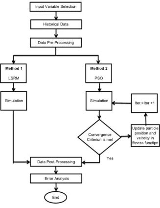
The MTLF procedure for the models can be viewed in Figure 1.

2.1. Data Source

Input variable selection, including: month type, peak load, average electrical de- mand, humidity and temperature data, and weather influences of previous time.

2.2. Historical Data

The monthly or weekly peak load demand data recorded from NEPCO for the years (2008-2014) taking into account external variables like holidays, weather and population growth.

2.3. Data Pre-Processing

It may be inevitable to have improperly recorded data and observation error.

Therefore the monthly and weekly reported data from NEPCO used to initialize the simulation results.

2.4. Simulation

In this part, the peak load forecasting output is simulated using Matlab.

2.5. Convergence Criteria

The stopping criterion is met when the parameters of PSO are achieving a global forecasting error within an efficient computation time. The convergence error must be less than 0.01% to make a sufficiently good fitness value.

2.6. Post Processing

The LSRM and PSO coefficients require calculations to prompt the desired fore-casted load results.

2.7. Error Analysis

As characteristics of load changes, error observations become more significant for the forecasting process. LSE is used to improve the accuracy of these models.

3. Forecasting Methodology

Regression analysis is widely used in the analysis of data for any design. Regres-sion models one of the most commonly used statistical analysis techniques in any research [6]. Typically, regression analysis is used to discover the relation-ships between a dependent variable and a set of independent variables based on a sample from input data [7]. We will study the method in the context of a re-gression problem, where the variation in one variable, called the response varia-ble Y, can be partly explained by the variation in the other variavaria-bles, called co-variables X. For example, variation in exam results Y are mainly caused by variation in abilities X of the students [8]. The least squares estimates used to minimize the error sum of squares:

(

)

^ 1

LSE n _{i i}

i= Y Y

=

∑

where: Yi: Actual load value in MW for week or month,

^ i

Y : Predicted load

value in MW for week or month, n: Number of samples (weeks or months).

3.1. Least Square Regression Methods

Regression analysis is the study of the action of the time series or process in the past and it is mathematical model, therefore the future behavior can be expected from it. In the forecasting process of medium term peak load, least squares regres-sion methods are used by different relations between the input and output [9].

3.1.1. Linear Regression

regres-sion method LRM model is designed to study the relationship between a pair of variables that appear in a data set. It is a model based on the linear relationship between the total demand y and month x as shown in Equations (2)-(4) [10].

y=ax b+ (2)

where: a: The slope, b: The interception point at y axis.

The least squares criterion is used to generate the line y=ax b+ that fits a

set of n data points.

By using the least square error approach [10], a and b coefficients can be

given by:

(

)(

)

(

)

(

)

(

) (

)

2

1 1 1

2 2

1 1

n n n

i i i i

i i i

n n

i

i i

x y x y x

a

n x x

= = = = = − = −

∑

∑

∑

∑

∑

(

) (

)(

)

(

) (

)

1 1

n n n

i i i i

i i i

n n

i

i i

n x y x y

b

n x x

= = = = = − = −

∑

∑

∑

∑

∑

where: n: The number of months which the forecasting is based on, yi: The

total load demand for all period for forecasting, xi: The total sum of months.

When a and b coefficients are obtained, the load forecasting is performed

by Equation (2.2).

3.1.2. Quadratic Regression

In this approach the parabolic function which is given in Equation (5) is used

2

.

y=ax +bx+c (5)

After applying least square error we can find a, b and c parameters in

matrix form [10].

4 3 2 2

3 2

2

i i i i i

i i i i i

i i i

x x x a x y

x x x b x y

x x n c y

 _{ }    _{  =}         _{ }      

∑

∑

∑

∑

∑

∑

∑

∑

∑

∑

∑

When a, b and c coefficients obtained the load forecasting is performed

by Equation (5).

3.1.3. Exponential Regression

In this method the exponential function is obtained through Equations (8)-(15) to get Equation (7).

x

y=ab (7)

By writing the equation in logarithmic form, the equation becomes:

log_y=log_abx. (8)

The properties of algorithms give

logy=loga+xlog .b (9)

This expresses logy as a linear function of x with slope.

Intercept=loga=A (11)

Therefore, if we find the best line using logy as A function the slope and

intercept will be gives as linear regression, so that the coefficients m and A

de-rives as linear equation.

(

)

(

)

(

)

(

)

(

)

(

)

i i i

i i

x y x

x x y x m n − = −

∑

∑

∑

∑

∑

(

) (

)(

)

(

)

(

)

i i i i

i i

x y x y

x n A n x − = −

∑

∑

∑

∑

∑

After linearization, a and b coefficients are shown in Equations (12) and

(13).

10A

a= (14)

10m

b= (15)

When a and b coefficients are obtained the load forecasting is performed

by Equation (7) [10].

3.2. Particle Swarm Optimization

A Particle swarm optimization PSO technique is used to find the optimal para-meters for different forecasting methods. This algorithm is used to solve a wide class of complex optimization problems in engineering and science. Both linear and nonlinear models will be used in the system and the results will be obtained using PSO. Through the implementation of PSO all particles are kept as mem-bers of the population. The basic idea of the PSO is the mathematical modeling and simulation of the food searching activities of a swarm of birds in the multi- dimensional space where the optimal solution is sought. Each particle in the swarm is moved towards a point where it obtains optimal solution by the influ-ence of its velocity. The velocity of a particle is affected by three factors; inertial momentum, cognitive and social [11]. The goal of PSO is to find the optimal va-riable values for a certain function. Each particle knows its optimal value (pbest)

and its velocity and position. Also, each particle knows the optimal value in the group (gbest) among pbests. Each particle seeks to adjust its position using the

current velocity and the distance obtained from the pbest and gbest. Based on

the above discussion, the mathematical model for PSO is represented as velocity update equation given by Equations (16)-(18).

(

)

(

)

1

1 1 2 2

k k k k k k

i i i i i i

v + =wv +c r pbest −x +c r gbest −x (16)

1 1

k k k

i i i

x+ =x +v+ (17)

where:

i

v: The velocity of particle.

i

x : The current position of particle.

1

c and c2 are positive constants, used to pull each particle to pbest and

best

1

r and r2 are two randomly generated numbers with a range [0 1].

w is the inertia weight and it keeps balance between exploration and

exploi-tation.

( )

max

Max.Iter.

w w

w k =w −  − _k

  (18)

min

w : The initial weight.

max

w : The final weight.

i

pbest : The best particle position i achieved. i

gbest : The best position of all particles achieved. k: The iteration index.

In this work, PSO is employed to minimize the LSE between the real values and prediction values. To evaluate the forecasting process for each model, LSE error can be used.

3.3. Auto Regressive (AR) Model

The AR model was developed by Box and Jenkins in 1970 to analyze historical data that had relations within it. In this study, the parameters were obtained from NEPCO. The AR process utilizes the least squares (LS) method, and it is an analogous way to fit a model by minimizing the sum of square errors for esti-mating parameters. The LSE uses the normal equations to implement the poly-nomial system. The parameters can be solved by Matlab. The purpose of this study was to implement the discounted least squares method with direct smoothing for estimating autoregressive model parameters [12].

The AR model structure is given by Equation (19)

( ) ( ) ( )

A q ∗y t =e t (19)

( )

A q : The parameters that are estimated using variants of the least-squares

method.

( )

y t : iddata object that contains the time-series data (one output channel).

( )

e t : Random Error.

The parameters of A q

( )

( )

1

1 i i i 1, 2, ,

i

A q a q− i q

=

= +

∑

i

a : The coefficients for each order.

q: Scalar that specifies the order of the model you want to estimate (the

number of A parameters in the AR model).

i

 : Random error.

4. Results and Discussions

for different forecasting models. Linear, quadratic, exponential and AR models are used in the system and the results obtained using PSO are compared with those of LSRM. A Matlab code was generated to execute the PSO Algorithm and LSRM Using the peak data of NEPCO grid. For PSO, all particles start at a ran-dom position in the range [0, 1] for each dimensions. The swarm size was li-mited to 250 particles. The selections of some parameters to carry out the pro-cedures of the work successfully has great effect on the model, these parameters are maximum speed, inertia weight and acceleration constants. The most suita-ble values for maximum speed is set to be 2, wmax and wmin are 0.9 and 0.4, C1

and C2 are 2.

Key parameters of PSO algorithm used in this paper are presented in Table 1.

4.1. Case One: MTLF Based on Peak Load Data

Peak Loads of NEPCO recorded in the years [2008-2014] are used to estimate the coefficients of linear, quadratic and exponential models for MTLF. The in-puts of these models are the number of weeks or months and the peak loads rec-orded in the years [2008-2014], whereas the output is the monthly or weekly peak loads predicted for the year 2015.

4.1.1. Monthly Forecasting

PSO and LSRM techniques are used to estimate models parameters. Horizon and the computed parameters are tabulated in Table 2.

Since the forecasting in this work is carried out on monthly bases, monthly least square error is performed and calculated by Equation (21). The equation used is given by:

Forecasted peak loads

LSE 1 100%

Actual peak loads

 

= −_{ }∗

  (21)

Table 1. PSO parameters.

Parameter Value

Population 250 particles Stop criterion 500 iterations Velocity Vmax = 2, Vmin = 0

Acceleration constants C1 = 2, C2 = 2

Inertia weight wmax = 0.9, wmin = 0.4

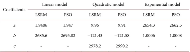
Table 2. Monthly estimated coefficients based on LSRM and PSO.

Coefficients Linear model Quadratic model Exponential model LSRM PSO LSRM PSO LSRM PSO a 1.9406 1.947 9.96 9.91 2654.3 2662.5 b 2685.6 2695.82 −121.43 −121.58 1.0006 1.0008

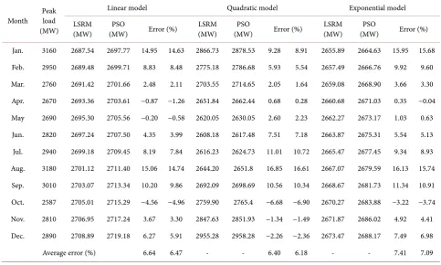
The monthly forecasted peak loads based on the parameters of linear, qua-dratic and exponential models and monthly least square error are shown in Ta-ble 3.

It can be concluded from the tables that the results computed by PSO are more close to the peak load and have less error. In both approaches, the monthly peak load is increased continuously from January till December when using li-near or exponential models. In quadratic model, the peak load is decreased con-tinuously from January till June and increased from June till December. The fo-recasted monthly peak load using different models are shown in Figure 2.

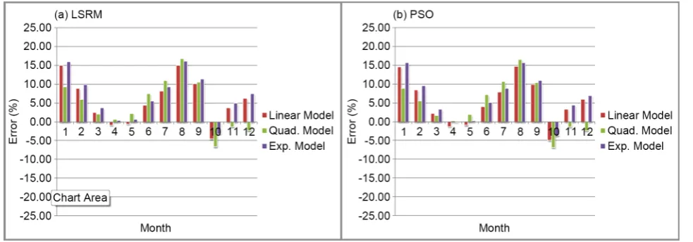
It can be seen from the figure that the PSO and LSRM are close to each other. In each model the difference between LSRM and PSO is arranged from [10][11] [12] MW. This difference make LSRM very close to the real peak load in April, May and October, otherwise the PSO achieves better estimation for the pre-dicted peak load. The results show that the PSO model is more accurate than LSRM and moreover, it is closer to the real peak load data for the year 2015. The monthly error performed by LSRM and PSO algorithm is shown in Figure 3.

From Figure 3, it can be observed that the Error for 2015 with LSRM and PSO is arranged from 0.04% to 16.85%. The Error less than 10% for nine months in LSRM and PSO approaches. The average error in LSRM for linear model is 6.64%, for quadratic model is 6.40%, and for exponential is 7.41%. So it can be seen that the best represented model between the months and peak load in LSRM is the quadratic regression model. The average error in PSO for linear model is 6.47%, for quadratic model is 6.18%, and for exponential is 7.09%.

Table 3. Monthly morning peak loads for the year 2015 compared with the actual readings.

Month Peak load (MW)

Linear model Quadratic model Exponential model LSRM

(MW) (MW) PSO Error (%) (MW) LSRM (MW) PSO Error (%) LSRM (MW) (MW) PSO Error (%) Jan. 3160 2687.54 2697.77 14.95 14.63 2866.73 2878.53 9.28 8.91 2655.89 2664.63 15.95 15.68 Feb. 2950 2689.48 2699.71 8.83 8.48 2775.18 2786.68 5.93 5.54 2657.49 2666.76 9.92 9.60 Mar. 2760 2691.42 2701.66 2.48 2.11 2703.55 2714.65 2.05 1.64 2659.08 2668.90 3.66 3.30 Apr. 2670 2693.36 2703.61 −0.87 −1.26 2651.84 2662.44 0.68 0.28 2660.68 2671.03 0.35 −0.04 May 2690 2695.30 2705.56 −0.20 −0.58 2620.05 2630.05 2.60 2.23 2662.27 2673.17 1.03 0.63 Jun. 2820 2697.24 2707.50 4.35 3.99 2608.18 2617.48 7.51 7.18 2663.87 2675.31 5.54 5.13 Jul. 2940 2699.18 2709.45 8.19 7.84 2616.23 2624.73 11.01 10.72 2665.47 2677.45 9.34 8.93 Aug. 3180 2701.12 2711.40 15.06 14.74 2644.20 2651.8 16.85 16.61 2667.07 2679.59 16.13 15.74

Figure 2. Monthly forecasted peak load using LSRM and PSO.

Figure 3. Monthly error associated with LSRM and PSO.

Therefore the best represented model between the months and peak load in PSO is the quadratic regression model.

4.1.2. Weekly Forecasting

Weekly real peak demands recorded in the years [2008-2014] are used in this section. The data set is used to establish an over determined system of equations. This system of equations is LSRM and PSO technique. The weekly real peak loads are used to find the coefficients for linear, quadratic and exponential mod-els. PSO and LSRM techniques are used to estimate models parameters for the same time horizon and the computed parameters are tabulated in Table 4.

The forecasted loads based on the parameters of linear, quadratic and expo-nential models and weekly least square error are shown in Table 5.

It can be concluded from the tables that the error computed by PSO are less than LSRM. In linear and exponential models, the weekly prediction load is in-creased from the first week till last week of the year 2015. In quadratic model, the weekly prediction load has vertex point [minimum peak value] occurs at week number 26. The peak load demand expected using LSRM and PSO shown

Table 4. Weekly estimated coefficients based on PSO and LSRM.

Coefficients Linear model Quadratic model Exponential model

LSRM PSO LSRM PSO LSRM PSO

a 0.8704 0.931 0.523 0.551 2524.8 2532.4

b 2531 2652.3 −26.8491 −26.95 1.0003 1.0005

c - - 2780.4 2794.6 - -

Table 5. Weekly peak loads for the year 2015 compared with the actual readings.

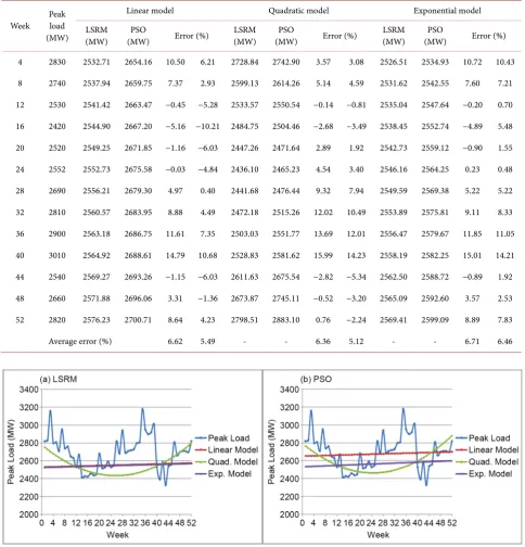
Week Peak load (MW)

Linear model Quadratic model Exponential model LSRM

(MW) (MW) PSO Error (%) LSRM (MW) (MW) PSO Error (%) LSRM (MW) (MW) PSO Error (%) 4 2830 2532.71 2654.16 10.50 6.21 2728.84 2742.90 3.57 3.08 2526.51 2534.93 10.72 10.43

8 2740 2537.94 2659.75 7.37 2.93 2599.13 2614.26 5.14 4.59 2531.62 2542.55 7.60 7.21

12 2530 2541.42 2663.47 −0.45 −5.28 2533.57 2550.54 −0.14 −0.81 2535.04 2547.64 −0.20 0.70

16 2420 2544.90 2667.20 −5.16 −10.21 2484.75 2504.46 −2.68 −3.49 2538.45 2552.74 −4.89 5.48

20 2520 2549.25 2671.85 −1.16 −6.03 2447.26 2471.64 2.89 1.92 2542.73 2559.12 −0.90 1.55

24 2552 2552.73 2675.58 −0.03 −4.84 2436.10 2465.23 4.54 3.40 2546.16 2564.25 0.23 0.48

28 2690 2556.21 2679.30 4.97 0.40 2441.68 2476.44 9.32 7.94 2549.59 2569.38 5.22 5.22

32 2810 2560.57 2683.95 8.88 4.49 2472.18 2515.26 12.02 10.49 2553.89 2575.81 9.11 8.33

36 2900 2563.18 2686.75 11.61 7.35 2503.03 2551.77 13.69 12.01 2556.47 2579.67 11.85 11.05

40 3010 2564.92 2688.61 14.79 10.68 2528.83 2581.62 15.99 14.23 2558.19 2582.25 15.01 14.21

44 2540 2569.27 2693.26 −1.15 −6.03 2611.63 2675.54 −2.82 −5.34 2562.50 2588.72 −0.89 1.92

48 2660 2571.88 2696.06 3.31 −1.36 2673.87 2745.11 −0.52 −3.20 2565.09 2592.60 3.57 2.53

52 2820 2576.23 2700.71 8.64 4.23 2798.51 2883.10 0.76 −2.24 2569.41 2599.09 8.89 7.83

Average error (%) 6.62 5.49 - - 6.36 5.12 - - 6.71 6.46

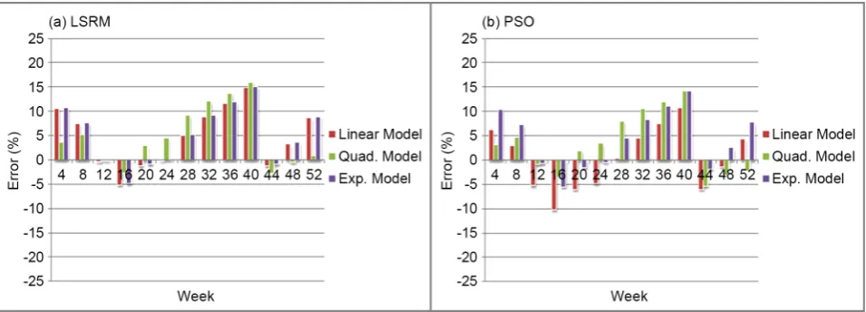
From Figure 4, it can be concluded that the PSO technique gives more accu-rate results than LSRM. In LSRM model, the prediction of the weekly peak load data gives results close to the real value in the weeks number 20, 24 and 44, oth-erwise the PSO technique represent the best model for all weeks in the year 2015. The weekly error performed by LSRM and PSO algorithm is shown in Figure 5.

From Figure 5, it can be seen that the error has minimum values for 20 weeks and maximum values for 10 weeks arranged from 0.0% to 15.99%. From average error point of view it is found that PSO method has produced better estimates than the LSRM and the quadratic model has the least error. Therefore, the best represented model between the weeks and peak load in LSRM and PSO is the quadratic regression model.

4.2. Case Two: MTLF Based on Weather Effect

Weather is the most important independent variable for MTLF. In this section, MTLF models used weather influence to predict the future peak load demand in terms of month and week. Various weather variables could be considered for MTLF. Temperature is the most commonly used for load predictors. The result of the previous section shows that there is a high positive correlation between temperature and peak load during summer and there is a negative correlation between temperature and peak load during winter. For these positive and nega-tive correlations, LSRM used to predict the peak load in the hot and cold days. Because the relation between temperature and peak load is very complicated in nature and cannot be analyzed with ordinary mathematical models, the qua-dratic model used for data obtained in summer and winter seasons.

4.2.1. Monthly Forecasting

Peak loads of NEPCO are used to estimate the coefficients of quadratic model for MTLF in summer and winter season. Summer season extends from June till September; winter season extends from December till March. Long studies in-vestigated that the changing of the temperature affects the peak load. The re-searches focused on the effect of the higher and lower temperatures on electricity

consumption using peak load data and temperature influence. The studies indi-cate that the impact of a one-degree in temperature higher than 25˚C, the peak load predicted will increase by 8 MW and a one-degree in temperature lower than 15˚C, the peak load predicted will increase by 6 MW [13].

The inputs of this model is the number of months per each season and the peak loads recorded in the years [2008-2014], whereas the output is the monthly peak loads predicted for the year 2015 after taking the temperature effect by each season. PSO and LSRM techniques are used to estimate quadratic model para-meters for winter and summer season. The quadratic parapara-meters are tabulated in

Table 6.

Table 7 represents the adjusted forecasted loads based on the parameters of

quadratic model after taking the temperature effect by each season and monthly least square error.

It can be concluded from the table that in summer season, the peak load is in-creased continuously from June till August and dein-creased from August till

Table 6. Monthly estimated coefficients for LSRM and PSO based on temperature effect.

Coefficients Summer Winter

LSRM PSO LSRM PSO

a 1.439 1.428 −55.07 −56.07 b 93.82 93.71 447.28 446.21

c 2536.2 2532 2144 2142

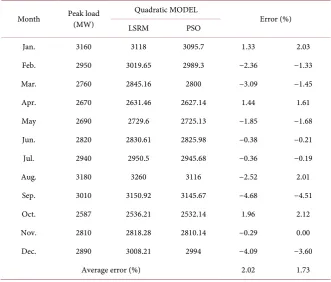
Table 7. Monthly forecasted peak load by quadratic model based on temperature effect.

Month Peak load _(MW) Quadratic MODEL Error (%) LSRM PSO

Jan. 3160 3118 3095.7 1.33 2.03 Feb. 2950 3019.65 2989.3 −2.36 −1.33 Mar. 2760 2845.16 2800 −3.09 −1.45 Apr. 2670 2631.46 2627.14 1.44 1.61 May 2690 2729.6 2725.13 −1.85 −1.68 Jun. 2820 2830.61 2825.98 −0.38 −0.21 Jul. 2940 2950.5 2945.68 −0.36 −0.19 Aug. 3180 3260 3116 −2.52 2.01

Sep. 3010 3150.92 3145.67 −4.68 −4.51 Oct. 2587 2536.21 2532.14 1.96 2.12 Nov. 2810 2818.28 2810.14 −0.29 0.00 Dec. 2890 3008.21 2994 −4.09 −3.60

September, while in winter season the peak load is increased continuously from December till January and decreased continuously from January till March. The forecasted monthly peak load using quadratic model and PSO algorithm based on temperature effect is shown in Figure 6.

It can be observed from Figure 6 that the results obtained by the PSO are very close to the real values and more accurate than the results obtained by LSRM. The prediction load obtained by LSRM is very close to the real peak load in Jan-uary, April and October, otherwise the PSO made better estimation for the pre-dicted peak load. Figure 7 is shown the monthly least square error based on temperature effect.

From Figure 7, it can be noticed that the error for 2015 with quadratic model and PSO algorithm is less than 5% for every month. The minimum error 0.0% is happened in November, while the maximum error 4.68% is happened in Sep-tember. The average error in Quadratic model is 2.02% and in PSO algorithm is 1.73%. Therefore, the PSO approach gives the best represented model between the months and peak load based on temperature effect.

4.2.2. Weekly Forecasting

The historical and weather data for the period [2008-2014] are used for estima-tion the models parameters for winter and summer seasons. Data for the year

Figure 6. Monthly peak load using quadratic model based on temperature effect.

2015 are used for testing LSRM and PSO models. The inputs of this model is the number of weeks per each season, whereas the output is weekly peak loads pre-dicted for the year 2015 after taking the temperature effect by each season. The quadratic parameters are tabulated in Table 8.

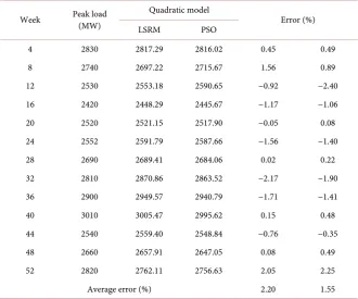
The weekly forecasted peak load using quadratic model and PSO algorithm based on temperature effect is shown in Figure 8.

From Figure 8, it can be noticed that the PSO results are very close to the real peak load data for the most weeks in the year 2015. The maximum peak loads in 2015 are happened in the weeks representing the summer and winter seasons, therefore the difference in values between real and prediction load data has the maximum in these weeks. The adjusted forecasted loads based on the parameters of quadratic model and weekly least square error are shown in Table 9.

It can be concluded from the table that in summer season, the peak load is in-creased continuously from the 22nd _{week till the 35}th _{week and decreased from}

the 36th _{week till the 39}th _{week (the weeks representing summer semester), while}

in winter season the peak load is increased continuously from the 48th _{week till}

the 3rd _{week and decreased continuously from the 4}th _{week till the 12}th _{week (the}

weeks representing the winter semester). The weekly least square error depends on the temperature effect is shown in Figure 9.

From Figure 9, it can be observed that the error has minimum values for 45 weeks and maximum values for 7 weeks arranged from 0.02% to 2.25%. The av-erage error in Quadratic model is 2.20% and in PSO algorithm is 1.55%. From

Table 8. Weekly estimated coefficients for LSRM and PSO based on temperature effect.

Coefficients Summer Winter

LSRM PSO LSRM PSO

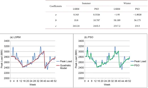
a 0.343 0.3326 −1.95 −1.8028 b 10.8 10.787 58.189 56.175 c 2412.8 2410.3 2317.2 2313

Figure 9. Weekly forecasting error using quadratic model based on temperature effect.

Table 9. Weekly forecasted peak load by quadratic model based on temperature effect.

Week Peak load _(MW) Quadratic model Error (%) LSRM PSO

4 2830 2817.29 2816.02 0.45 0.49 8 2740 2697.22 2715.67 1.56 0.89 12 2530 2553.18 2590.65 −0.92 −2.40 16 2420 2448.29 2445.67 −1.17 −1.06 20 2520 2521.15 2517.90 −0.05 0.08 24 2552 2591.79 2587.66 −1.56 −1.40 28 2690 2689.41 2684.06 0.02 0.22 32 2810 2870.86 2863.52 −2.17 −1.90 36 2900 2949.57 2940.79 −1.71 −1.41 40 3010 3005.47 2995.62 0.15 0.48 44 2540 2559.40 2548.84 −0.76 −0.35 48 2660 2657.91 2647.05 0.08 0.49 52 2820 2762.11 2756.63 2.05 2.25 Average error (%) 2.20 1.55

average error point of view it is found that PSO method has produced better es-timation than the LSRM.

4.3. MTLF Using AR Model

4.3.1. Monthly Forecasting Using AR Model

Monthly real peak demands recorded in the years [2008-2014] are used to im-plement AR model and the real data for 2015 is used to test this model. The monthly AR model parameters which are estimated using variants of the least- squares method are given by the following equation.

( )

6 7 8 9

10 11 12 13

1 0.2104 0.03418 0.2267 0.1482 0.1307

0.1791 0.2062 0.05049 0.2337

0.0805 0.3338 0.2585 0.198

A q q q q q q

q q q q

q q q q

− − − − −

− − − −

− − − −

= − − − + −

− + + +

− − − +

(22)

The monthly forecasted loads based on the parameters of AR model and monthly least square error are shown in Table 10.

It can be concluded from the table that the error computed by AR model is high compared with other techniques. In February, March and May the AR model gives good results, otherwise the results gives unacceptable prediction of peak load data. By using Equation (19) in Matlab, The monthly forecasted peak load using AR model can be shown in Figure 10.

From Figure 10, it can be observed that the difference between the results ob-tained by AR model for monthly peak load and the real data is relatively high. This difference makes an average error high compared with the LSRM and PSO techniques used in previous section. The monthly least square error using AR model is shown in Figure 11.

From Figure 11, it can be observed that the error is very high shown in 6 months for the year 2015. The AR model gives the maximum error 17.96% in January while gives the minimum error 2.35% in March with an average error equal to 8.88% for this model.

Table 10. Monthly forecasted peak load using AR model.

Month Peak load (MW) AR (MW) Error (%)

Jan. 3160 2592.40 17.96

Feb. 2950 2858.26 3.11

Mar. 2760 2695.13 2.35

Apr. 2670 2852.50 −6.84

May 2690 2758.84 −2.56

Jun. 2820 2442.88 13.37

Jul. 2940 2645.44 10.02

Aug. 3180 2784.94 12.42

Sep. 3010 2811.21 6.60

Oct. 2587 2957.33 −14.32

Nov. 2810 2666.22 5.12

Dec. 2890 2547.89 11.84

Figure 10. Monthly peak load using AR model.

Figure 11. Monthly forecasting error using AR model.

4.3.2. Weekly Forecasting Using AR Model

Weekly real peak demands recorded in the years [2008-2014] are used in this section. The data set is used to establish AR model. The weekly AR model para-meters which are estimated using variants of the least-squares method are given by the following equation.

( )

6 7 8 9 10

11 12 13

1 0.1912 0.1514 0.0119 0.1326 0.0704

0.06091 0.06546 0.0622 0.04643 0.09075

0.05682 0.07205 0.01145

A q q q q q q

q q q q q

q q q

− − − − −

− − − − −

− − −

= − − + − −

− − − − −

− − −

(23)

The weekly forecasted loads using AR model and weekly least square error are shown in Table 11.

a big difference compared with real value shown in many weeks for this year. By using Equation (19) in Matlab, The weekly forecasted peak load using AR model can be shown in Figure 12.

From Figure 12, it can be noticed that the results obtained by AR have a big difference with the real peak load data for the most weeks in the year 2015, therefore the difference in values between real and prediction load data has maximum for this model. The weekly least square error using AR model is shown in Figure 13.

Table 11. Weekly forecasted peak load using AR model.

Week Peak load (MW) AR (MW) Error (%)

4 2830 2659.93 6.01

8 2740 2692.87 1.72

12 2530 2691.63 −6.39

16 2420 2686.27 −11.00

20 2520 2686.21 −6.60

24 2552 2684.31 −5.18

28 2690 2684.72 0.20

32 2810 2683.94 4.49

36 2900 2683.42 7.47

40 3010 2683.23 10.86

44 2540 2682.58 −5.61

48 2660 2682.15 −0.83

52 2820 2681.49 4.91

Average error (%) 8.12

Figure 13. Weekly forecasting error using AR model.

From Figure 13, it can be observed that the error has minimum values for 10 weeks and maximum values for 25 weeks arranged from 0.2% to 18.99%. From average error point of view it is found that AR model has produced least esti-mates than the LSRM and PSO with an average error equal to 8.12%.

5. Conclusion

Table 12. The monthly and weekly average error for each model covered in this work (%).

Forecasting type

Forecasting depends on peak load

Forecasting depends on peak load adjusted

considering weather

effects Forecasting _{by using} AR model Linear model Quadratic model Exponential model Quadratic model

LSRM PSO LSRM PSO LSRM PSO LSRM PSO

Monthly 6.64 6.47 6.40 6.18 7.41 7.09 2.02 1.73 8.88

Weekly 6.62 5.49 6.36 5.12 6.71 6.46 2.20 1.55 8.12

effects. The average error for LSRM and PSO for the three models and forecast-ing usforecast-ing AR model are represented in Table 12.

References

[1] Alfares, H. and Nazeeruddin, M. (2002) Electric Load Forecasting: Literature Survey and Classification of Methods. International Journal of Systems Science, 33, 23-34. https://doi.org/10.1080/00207720110067421

[2] Chow, J., Wu, F. and Momoh, J. (2005) Applied Mathematics for Restructured Electric Power Systems. Springer, New York.

[3] Hahn, H., Meyer-Nieberg, S. and Pickl, S. (2009) Electric Load Forecasting Me-thods: Tools for Decision Making. European Journal of Operational Research, 199, 902-907. https://doi.org/10.1016/j.ejor.2009.01.062

[4] Espinoza, M., Suykens, J., Belmans, R. and De Moor, B. (2007) Electric Load Fore-casting-Using Kernel Based Modeling for Nonlinear System Identification. IEEE Control Systems Magazine Special Issue on Applications of System Identification, 27, 43-57.

[5] NEPCO (2016) Private Communication. http://www.nepco.com.jo/en/Default_en.aspx

[6] Schachter, J. and Mancarella, P. (2014) A Short-Term Load Forecasting Model for Demand Response Applications. 11th International Conference on the European Energy Market, Krakow, 28-30 May 2014, 1-5.

https://doi.org/10.1109/EEM.2014.6861220

[7] Ding, C.S. (2006) Using Regression Mixture Analysis in Educational Research. Practical Assessment Research & Evaluation, 11, 1-11.

[8] Van De Geer, S.A. (2005) Least Squares Estimation. Encyclopedia of Statistics in Behavioral Science, 2, 1041-1045.

[9] Willis, H. and Northcote-Green, J.D. (1984) Comparison Tests of Fourteen Distri-bution Load Forecasting Methods. IEEE Transactions on Power Apparatus and Systems, 103, 1190-1197.https://doi.org/10.1109/TPAS.1984.318448

[10] Canale, P. (2006) Numerical Methods for Engineers. 6th Edition, McGraw-Hill Science, New York, 451-484.

[11] Tomar, S.K. and Prasad, R. (2009) Conventional and PSO Based Approaches for Model Order Reduction of SISO Discrete Systems. International Journal of Electric-al and Electronics Engineering, 2, 45-50.

Sys-tems, 2, 122-135.

[13] Momani, M., Yatim, B. and Ali, M. (2009) The Impact of the Daylight Saving Time on Electricity Consumption—A Case Study from Jordan. Energy Policy, 37, 2042- 2051.https://doi.org/10.1016/j.enpol.2009.02.009

Submit or recommend next manuscript to SCIRP and we will provide best service for you:

Accepting pre-submission inquiries through Email, Facebook, LinkedIn, Twitter, etc. A wide selection of journals (inclusive of 9 subjects, more than 200 journals)

Providing 24-hour high-quality service User-friendly online submission system Fair and swift peer-review system

Efficient typesetting and proofreading procedure

Display of the result of downloads and visits, as well as the number of cited articles Maximum dissemination of your research work