Developing an Integrated Complementary Relationship for Estimating Evapotranspiration

http://www.scirp.org/journal/nr ISSN Online: 2158-7086 ISSN Print: 2158-706X

DOI: 10.4236/nr.2018.94007 Apr. 17, 2018 89 Natural Resources

Developing an Integrated Complementary

Relationship for Estimating Evapotranspiration

Homin Kim

_{, Jagath J. Kaluarachchi}

1_{Utah Water Research Laboratory, Utah State University, Logan, UT, USA}

2_{College of Engineering, Utah State University, Logan, UT, USA}

Abstract

The complementary relationship for estimating evapotranspiration (ET) is a simple approach requiring only commonly available meteorological data; however, most complementary relationship models decrease in predictive power with increasing aridity. In this study, a previously developed Granger and Gray (GG) model by using Budyko framework is further improved to es-timate ET under a variety of climatic conditions. This updated GG model, GG-NDVI, includes Normalized Difference Vegetation Index (NDVI), preci-pitation, and potential evapotranspiration based on the Budyko framework. The Budyko framework is consistent with the complementary relationship and performs well under dry conditions. We validated the GG-NDVI model under operational conditions with the commonly used remote sensing-based Operational Simplified Surface Energy Balance (SSEBop) model at 60 Eddy Covariance AmeriFlux sites located in the USA. Results showed that the Root Mean Square Error (RMSE) for GG-NDVI ranged between 15 and 20 mm/month, which is lower than for SSEBop every year. Although the magni-tude of agreement seems to vary from site to site and from season to season, the occurrences of RMSE less than 20 mm/month with the proposed model are more frequent than with SSEBop in both dry and wet sites. Another find-ing is that the assumption of symmetric complementary relationship is a defi-ciency in GG-NDVI that may introduce an inherent limitation under certain conditions. We proposed a nonlinear correction function that was incorpo-rated into GG-NDVI to overcome this limitation. As a result, the proposed model produced much lower RMSE values, along with lower RMSE across more sites, as compared to SSEBop.

Keywords

Evapotranspiration, NDVI, Complementary Relationship, SSEBop How to cite this paper: Kim, H. and

Ka-luarachchi, J.J. (2018) Developing an Inte-grated Complementary Relationship for Estimating Evapotranspiration. Natural Re-sources, 9, 89-109.

https://doi.org/10.4236/nr.2018.94007

Received: February 24, 2018 Accepted: April 14, 2018 Published: April 17, 2018

Copyright © 2018 by authors and Scientific Research Publishing Inc. This work is licensed under the Creative Commons Attribution International License (CC BY 4.0).

http://creativecommons.org/licenses/by/4.0/

DOI: 10.4236/nr.2018.94007 90 Natural Resources

1. Introduction

According to the U.S. Geological Survey (USGS) Famine Early Warning Systems Network [1], the rate and amount of evapotranspiration (ET) plays a considera-ble role in the monitoring of water loss from agricultural lands. As noted by Se-nay et al.[2], ET may be used to show the current vegetation condition com-pared to the historical records. This comparison has the potential to help identi-fy vegetation stress in time and space. ET estimation methods can be divided in-to two types: (1) ground-based ET methods that use standard meteorological data; and (2) ET models that use remote sensing data that must be combined with retrieval algorithms to estimate ET.

McMahon [3] classified the ground-based ET methods into six classes on the basis of application: 1) potential evapotranspiration (ETP); 2) reference evapo-transpiration; 3) actual evapoevapo-transpiration; 4) open water evaporation; 5) lake/ storage evaporation; and 6) pan evaporation. We have focused on actual ET in this study because it can be representative of actual conditions, whereas refer-ence evapotranspiration would require a vegetation resistance parameter and deep lakes would require water temperature data. In addition, we use the term “evapotranspiration (ET)” in this paper to include actual evapotranspiration ex-cept in places where the term “reference (crop) evapotranspiration” is used by other authors.

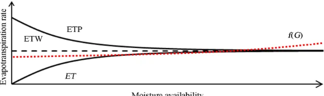
One approach to estimating ET with ground-based methods is the comple-mentary relationship proposed by Bouchet [4]. The primary advantage of the complementary relationship is that it generally requires only meteorological da-ta. Bouchet [4] suggested that as a surface dries, the decrease in ET is matched with an increase in potential evapotranspiration (ETP) as shown in Figure 1. Such a relationship offers a simple and attractive approach for estimating ET using ETP without the detailed knowledge of surface properties. Examples of widely known models using this concept are the Advection-Aridity (AA) model by Brutsaert [5], the Complementary Relationship Areal Evapotranspiration (CRAE) by Morton [6], and the GG model proposed by Granger [7]. These three models have been widely applied to a broad range of surface and atmospheric conditions [8][9][10][11][12].

Granger [13], however, argued that the symmetric relationship in Bouchet [4]

DOI: 10.4236/nr.2018.94007 91 Natural Resources

lacked a theoretical background and proved that the symmetric condition is only true when the temperature is near 6˚C. Hence, the author developed a new com-plementary relationship with the psychrometric constant and the slope of the saturation vapor pressure curve. Later, Crago [14] showed that the radiometric surface temperature measurements can be successfully incorporated into Gran-ger [13] equation. Similar to Crago [14], Anayah [15] proposed a modified ver-sion of the GG model using Priestley [16] equation instead of Penman [17] equ-ation. The model proposed by Anayah [15] is hereafter called the modified GG model. The results of the modified GG model showed a decrease in Root Mean Square Error (RMSE) from 20% to as much as 80% compared to the recent stu-dies of Mu [18], Mu [19], Han [20], and Thompson et al. [21]. On the other hand, Kahler [10] proposed an empirical constant, b, in Bouchet [4] hypothesis and demonstrated that b is generally greater than 1, based on their theoretical and experimental evidence, while the symmetric condition of Bouchet [4] hypo-thesis requires b = 1. More recently, Aminzadeh [22] extended the asymmetric complementary relationship with an analytical prediction of b for Kahler [10]. Furthermore, Venturini [23][24] applied surface temperature of Moderate Res-olution Imaging Spectroradiometer (MODIS) data into the GG model and showed a good agreement between their approach and measured ET. Especially, Szilagyi [25] developed a calibration free version of the complementary rela-tionship.

DOI: 10.4236/nr.2018.94007 92 Natural Resources

with estimated ET, showing a correlation coefficient of 60% compared to 37% in Allam [30].

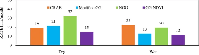
Figure 2 presents the results obtained from Kim [26]. These results are in agreement with Anayah [15], which showed that the modified GG model needs further improvements in dry conditions, and showed the lowest mean RMSE in both dry and wet sites. Overall, these results indicate that, among the ground- based methods [26], model can be used as a powerful methodology to estimate ET.

While these findings are good within the realm of complimentary methods (or ground-based methods), some of the more commonly used ET estimation me-thods now use remote sensing data. If the complementary relationship and the corresponding methods, such as the model proposed by Kim [26], are to be ac-cepted as operational models in field conditions, then the results should be compared and validated with remote sensing-based ET estimation methods. Taking into consideration of the improvements made with complementary rela-tionship-based methods, this study examines the work of Kim [26] in compari-son with a commonly used remote sensing method and measured ET data from 60 EC flux tower sites located across the USA.

Biggs et al.[31] grouped the remote sensing-based methods into three classes: vegetation-based methods, radiometric land surface temperature-based me-thods, and triangle/trapezoid or scatterplot inversion methods. Among them, the radiometric land surface temperature-based methods have a number of attrac-tive features compared to the other classes: minimal ground data, ease of imple-mentation, and operational application over large areas.

Radiometric land surface temperature-based methods use the fact that ET is a change of state in water that uses energy in the environment for vaporization and reduces surface temperature [32]. A subset of these methods is often called energy balance methods since they solve the energy balance equation. Moreover, these methods do not directly measure ET but must be combined with retrieval algorithms since data and technical requirements to solve the full energy balance equation can be challenging, especially in large regions. For example, the Surface Energy Balance Algorithm for Land (SEBAL) model [33][34] requires the mea-surements of wind speed, iterative calibration, and review by an expert operator. Mapping EvapoTranspiration at high Resolution with Internalized Calibration

Figure 2. Comparison of RMSE (mm/month) between different complementary rela-tionship models for 29 dry and 30 wet sites in the US. NGG and GG-NDVI refer to the models of Han [20] and Kim [26], respectively.

19 21 22

13 32

20 15

12

0 10 20 30 40 50

Dry Wet

R

M

S

E

[

mm/

mo

n

th

DOI: 10.4236/nr.2018.94007 93 Natural Resources

(METRIC) [35] needs high-quality meteorological data such as net radiation, air temperature, wind speed, and humidity. According to Allen [35], METRIC has higher accuracy for hourly reference ET than SEBAL, but the processing cost of METRIC is high.

As an alternative, FWESNET (USGS) has produced ET measurements from MODIS using the operational Simplified Surface Energy Balance (SSEBop) model [2]. The SSEBop setup uses the Simplified Surface Energy Balance (SSEB) approach developed by Senay [36]. The SSEB approach estimates ET using ET fraction scaled from thermal imagery in combination with a spatially explicit maximum reference ET. SSEB has an advantage in that it does not require air temperature and the knowledge of land cover types. Instead, the method uses the “hot” and “cold” pixel approach of Bastiaanssen [33] to calculate the ET fraction. Later, Senay [37] enhanced SSEB to accommodate diverse vegetation and topo-graphic conditions using a lapse rate correction factor. They successfully eva-luated the results by comparing with METRIC and ET values computed from the water balance approach. As a result of the work by Senay [37], the enhanced SSEB model increased the correlation with METRIC from 0.83 to 0.90. Fur-thermore, Senay et al.[38] proposed a revised SSEB to handle both elevation and latitude effects on surface temperature using the difference between Land Sur-face Temperature (LST) and air temperature. Recently, Senay et al.[2] proposed an operational SSEB, renamed as SSEBop, which uses predefined boundary con-ditions for hot and cold reference pixels so that ET can be calculated as a func-tion of LST and reference ET. The SSEBop approach has been validated com-prehensively by comparing with 45 EC flux tower observations [2] and then with both MOD16 and 60 EC flux tower observations [39]. Later, Bastiaanssenet al. [40] applied SSEBop to determine ET in the Nile Basin, Ethiopia, for mapping water production and consumption zones. SSEBop ET data is now freely availa-ble through the USGS Geo Data Portal.

Despite the general consensus of using SSEBop for estimating ET, a detailed study of SSEBop conducted by Senay et al.[2] showed that the use of reference ET can introduce a significant difference of up to 20% in the magnitude of ET. They also showed that the use of constant pre-defined differential temperature between the hot and cold boundary conditions can also create an inherent inac-curacy. Thus, it is important that SSEBop ET be validated and calibrated with available data such as EC flux tower data before using it to model ET.

DOI: 10.4236/nr.2018.94007 94 Natural Resources

2. Methodology and Data

2.1. Methodology

GG-NDVI is the most updated model using the original GG model. GG-NDVI uses historical annual Normalized Difference Vegetation Index (NDVI) data and precipitation to improve the ET estimates of the modified GG model proposed by Anayah [15]. We then used the SSEBop model (Senay et al.[2]) to further va-lidate GG-NDVI in comparison to an operational remote sensing model.

2.1.1. GG-NDVI Model

The first complementary relationship was proposed by Bouchet [4], who post-ulated that, as a surface dries, the actual ET decrease is matched by an equivalent increase in ETP. In spite of the fact that ET is negatively correlated with ETP, Morton [6] showed that the relationship has no defined shape. Granger [13] showed that the symmetrical relationship between ET and ETP only occurs when the temperature is near 6˚C and suggested the following complementary relationship formulation:

ET+

γ

γ

∆  ∆ (1)

where ET, ETP, and ETW are in mm/day, γ is the psychrometric constant (kPa/˚C), and ∆ is the slope of saturation vapor pressure-temperature (kPa/˚C) relationship. Thereafter, [7] developed the GG model based on Equation (1) us-ing the concept of relative evaporation. Recently, Anayah [15] developed the modified GG model using the work of Granger [7]. The performance of the modified GG model improves when the Priestley [16] equation shown in Equa-tion (2) is used to calculate ETW instead of Penman [17].

(

)

ETW

α

γ

∆ ∆

= −

+ (2)

where α is a coefficient equal to 1.28, Rn−Gsoil is net radiation (mm/day), and

soil

G is soil heat flux density (mm/day). Note that soil heat flux density is

neg-ligible compared to net radiation when calculated at daily or monthly time-scale [9].

ET is then estimated as a fraction of ETW using Equation (3): 2

ET ETW

1

G G

=

+ (3)

where G is the relative evaporation parameter derived from [7]. They proposed a unique relationship with a parameter called relative drying power (D). The unique relationship between G and D are described in Equations (4) and (5), re-spectively.

8.045

ET 1

ETP 1 0.028e D

G= =

DOI: 10.4236/nr.2018.94007 95 Natural Resources a

a n

E D

E R

=

+ (5)

where Ea is drying power of air (mm/day) given in Equation (6).

(

)

(

)

0.35 1 0.54

a s a

E = + U e −e (6)

where U is wind speed at 2 m above ground level (m/s), which is adjusted using the work of Allen [41]; es is saturation vapor pressure (mmHg); and ea is

vapor pressure of air (mmHg).

The performance of the GG model, including the modified GG model pro-posed later, decreased with increasing aridity. A possible reason is G in Equation (4), which was empirically derived from 158 sites representing wet environments in Canada. To improve the parameter G, GG-NDVI model (Kim [26]) used the latest version of the Fu equation (Li [27]). In particular, the Fu [42] equation is one of the formulations of the Budyko curve [43] and it is consistent with the complementary relationship [28][29]. The corresponding analytical formulation of the Fu equation is given in Equation (7).

1 ET

1 1

ETP ETP ETP

P   P ϖ ϖ = + − + _{ } 

 

 

  (7)

where P is precipitation (mm) and ETP is estimated using Penman [17]. Para-meter ϖ is a constant and represents the land surface conditions of the basin, especially the vegetation cover [27]. Furthermore, Li [27] showed that ϖ is li-nearly correlated with the long-term average annual vegetation cover that can help improve ET estimates. Reference Yang et al. [44] showed that vegetation cover defined by M is calculated using Equation (8).

min

max min

NDVI NDVI NDVI NDVI

M = −

− (8)

where NDVImin and NDVImax are chosen to be 0.05 and 0.8, respectively. An

op-timal 𝜛𝜛 value for the basin can be derived through a curve fitting procedure that minimizes RMSE between the measured and predicted evaporation ratio [27].

Li [27] proposed parameterization that is simply a linear regression between optimal ϖ and the long-term average M given as

a M b

ϖ

DOI: 10.4236/nr.2018.94007 96 Natural Resources

shows the Fu equation with the updated G now defined as Gnew. 1

ET P P

1 1

ETP ETP ETP

new

G

ϖ ϖ

 _{ } 

= = + − + _{ } 

 

 

  (10)

Note Gnew is the updated definition of relative evaporation, G, which

in-cludes the Budyko hypothesis and the vegetation index. To estimate Gnew, ETP

is required and can be estimated using Equation (11) [17].

(

)

ETP R_n G_soil

γ

γ

γ

∆ _{− +}

+∆ +∆

= (11)

Having found Gnew from Equation (11) and estimated ETW from Equation

(2), we can estimate ET of the proposed model from Equation (12). 2

ET ETW

1

new

new G G

=

+ (12)

2.1.2. SSEBop Model

The SSEBop algorithm (Senay et al.[2]) does not solve the full energy balance equation. This approach assumes that for a given time and location, the temper-ature difference between the hot and cold reference values of each pixel remains nearly constant throughout the year under clear sky conditions. Furthermore, the major simplification of SSEBop is based on the knowledge that the surface energy balance process is mostly driven by net radiation. With this simplifica-tion, the ET fracsimplifica-tion, ETf, is calculated using Equation (13).

ETf Th Ts Th Ts

dT Th Tc

− −

= =

− (13)

Here, ETf is between 0 and 1, with negative ETf values set to zero; Ts is sur-face temperature derived from MODIS LST; Th is hot reference value representing the temperature of hot conditions; and Tc is the cold reference val-ue derived as a fraction of maximum air temperature [2]. The difference between Th and Tc is dT with temperature units in Kelvin.

ET is estimated using Equation (14) as a fraction of reference ET.

o

ET=ETf×kET (14)

where ETo is reference ET, which is calculated from the Penman-Monteith

equa-tion [45][46], and k is a coefficient that scales ETo into the level of maximum ET

experienced by an aerodynamically rougher crop. A recommended value of k for the United States is 1.2.

2.2. Data

First, we used the SSEBop ET data set from the USGS Geo Data Portal

DOI: 10.4236/nr.2018.94007 97 Natural Resources

Among these, net radiation (Rn) was calculated using the equations recom-mended by Allen [45], similar to the SSEBop model. Air temperature, elevation, and precipitation data were obtained from the Parameter-elevation Regressions on Independent Slopes Model (PRISM) (http://www.prism.oregonstate.edu/, last accessed on Nov 23, 2015). As part of the input data for the GG-NDVI method, we used the 16-day Normalized Difference Vegetation Index (NDVI) data from MODIS (http://daac.ornl.gov/MODIS/modis.shtml, last accessed on Oct 23, 2015).

We collected the level 4 meteorological data including latent heat flux (LE) from 76 AmeriFlux stations (Oak Ridge National Laboratory’s AmeriFlux web-site, http://ameriflux.ornl.gov/, last accessed on Nov 23, 2015) then, we excluded those stations with actual vegetation type different from the MODIS global land cover product (MOD12) at any of surrounding 500 m by 500 m spatial resolu-tion. Also, we further excluded those stations with fewer than half a year of measurements during 2000-2007. As a result, 60 stations were used in this study as shown in Figure 3. The measured monthly latent heat flux data were used to calculate the corresponding ET using latent heat of vaporization of water.

We defined the climate class of each site using the aridity index of the United Nations Environment Programme (UNEP) proposed by Barrow [47]. The aridi-ty index divided climate conditions to six classes: hyper-arid, arid, semi-arid, dry sub-humid, wet sub-humid, and humid. However, this work simplified the cli-mate class definition to two classes, similar to the work of Anayah [15]: dry and wet. Using this simplification, 24 sites were identified as dry, compared to 36 sites under the wet class.

3. Results and Discussion

This study was conducted in two phases. Phase 1 is the validation stage in which comparisons are made between the SSEBop model and measured ET to assess the accuracy of the remote sensing method to estimate ET. In Phase 2, a com-parison of estimated ET from GG-NDVI with observed data will be performed

DOI: 10.4236/nr.2018.94007 98 Natural Resources

to identify the weaknesses of the GG-NDVI model, especially relative to the complementary relationship, and appropriate corrections will be proposed.

3.1. Phase 1: Validation of GG-NDVI

Capturing inter-annual variations of ET estimates is important. Although such variations are not significant when water is unlimited, estimating these varia-tions in water-limited condivaria-tions is essential for water resources management. In this phase, ET has been estimated from both SSEBop and GG-NDVI and com-pared against measured monthly ET data from 2000 to 2007.

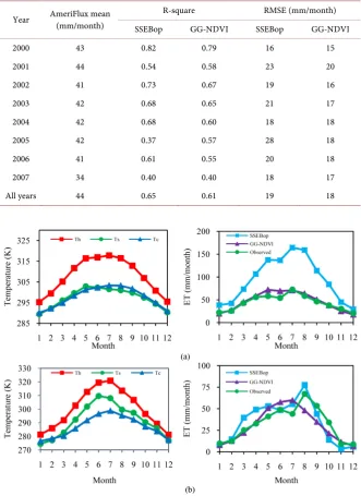
Table 1 presents the yearly comparison of results between the SSEBop and GG-NDVI estimates. Compared with measured ET, the results indicate that the accuracy of SSEBop and GG-NDVI estimates show satisfactory R-square and RMSE values. R-square values for SSEBop and GG-NDVI are 0.65 and 0.61, re-spectively. The results demonstrate that the ET estimates from GG-NDVI ET at an annual time-scale are reasonable. Figure 4, however, shows the 1:1 scatter of yearly variability of both models with GG-NDVI showing a tendency to unde-restimate in the higher ET range. In contrast, SSEBop tends to oveunde-restimate ET in the same higher ET range. Generally, higher ET occurs mostly in wet condi-tions, and underestimating ET in moist regions is a characteristic of the com-plementary relationship [9][48][49].

Figure 5 shows the poor results of SSEBop with the temporal variation in Th, Tc, and Ts on the left and the corresponding SSEBop, GG-NDVI, and measured ET values on the right. For example, at Austin Cary in Florida (Figure 5(a)), RMSE ranged from 29 to 164 mm/month for SSEBop and 17 to 70 mm/month for GG-NDVI. Moreover, SSEBop showed significant deviations from measured ET throughout the year, and RMSE varied from 29 to 164 mm/month. Where SSEBop shows low RMSE values in Figure 5(a) and Figure 5(b), a possible rea-son for these significant deviations could be the concept of ET faction (ETf) in SSEBop. ETf is calculated using Th, Tc, and Ts, and the Ts curve lies mostly be-tween the boundary conditions (Th and Tc). However, Ts in Figure 5(a) is close

Figure 4. Validation results of monthly ET estimates form SSEBop and GG-NDVI against AmerFlux ET data between 2000 and 2007.

0 50 100 150 200

0 20 40 60 80 100 120 140 160 180 200

Observed ET [mm/month]

SSE B o p E T [ m m /m o nt h]

R2 _{= 0.65}

0 50 100 150 200

0 20 40 60 80 100 120 140 160 180 200

Observed ET [mm/month]

G G -N D V I E T [m m /m o n th ]

DOI: 10.4236/nr.2018.94007 99 Natural Resources

Table 1. Comparison of monthly ET estimates between SSEBop and GG-NDVI using AmeriFlux data from 2000 to 2007.

Year AmeriFlux mean _(mm/month) R-square RMSE (mm/month) SSEBop GG-NDVI SSEBop GG-NDVI

2000 43 0.82 0.79 16 15

2001 44 0.54 0.58 23 20

2002 41 0.73 0.67 19 16

2003 42 0.68 0.65 21 17

2004 42 0.68 0.60 18 18

2005 42 0.37 0.57 28 18

2006 41 0.61 0.55 20 18

2007 34 0.40 0.40 18 17

All years 44 0.65 0.61 19 18

Figure 5. Temporal variation of 8-day average Ts, Th, Tc (left) and monthly ET estimates from SSEBop and GG-NDVI and measured ET at (a) Austin Cary in Florida and (b) Flagstaff in Arizona for 2005.

to the predefined cold boundary (Tc), which brings ETf closer to 1.0, resulting in a corresponding ET that is close to the maximum ET.

DOI: 10.4236/nr.2018.94007 100 Natural Resources

(a)

(b)

Figure 6. Histogram of RMSE (mm/month) of SSEBop and GG-NDVI for (a) dry and (b) wet sites.

is more frequent than with SSEBop in both dry and wet sites. The averages of RMSE across 24 dry sites for GG-NDVI and SSEBop are 19 mm/month and 22 mm/month, respectively. For 36 wet sites, GG-NDVI and SSEBop showed an average RMSE of 17 mm/month and 20 mm/month, respectively. These results indicate that GG-NDVI ET estimates improve with wetness, which is similar to the previous studies of Hobbins [9], Xu [12], and Anayah [15].

DOI: 10.4236/nr.2018.94007 101 Natural Resources

Figure 7. Comparisons of monthly ET between SSEBop and GG-NDVI against measured ET (a) and

time-series of NDVI at Brookings in South Dakota (b).

to Yang et al.[44], the relative infiltration capacity and the average topographic slope need to be taken into consideration when using the Fu equation, especially in small catchments. Therefore, more work is needed to generalize the relation-ship for the use of NDVI with changing vegetation cover within the Budyko framework. The next section will discuss options to improve the GG-NDVI model.

3.2. Phase 2: Enhancement to GG-NDVI

As described earlier, GG-NDVI performed slightly better than SSEBop in both dry and wet climate conditions, and GG-NDVI increased the predictive power with increasing humidity. One interesting finding is that RMSE from GG-NDVI increases slightly with the relative evaporation parameter as shown in Figure 8. Considering this observation, Phase 2 then focused on the relationship between the performance of GG-NDVI and Gin the context of using the complementary relationship.

DOI: 10.4236/nr.2018.94007 102 Natural Resources

Figure 8. RMSE from GG-NDVI versus relative evaporation (G = ET/ETP).

( )

2

ET ETW

1

new

new G

f G G

= × ×

+ (17)

where f(G) is the correction function. We expect the correction function to be nonlinear, similar to an exponential function, since the magnitude of the differ-ence between ET and ETW decreases exponentially as shown in Figure 1. In this work, we fitted 2772 data points to an exponential function similar to Equation (18). Multiple regression analysis was conducted to compute the values of the α and β coefficients.

( )

f G =

α

Regression analysis found that α is 0.7895 and β is 0.9655. Hereafter, the GG-NDVI model with the proposed correction function given as Equation (17) is called the Adjusted GG-NDVI model.

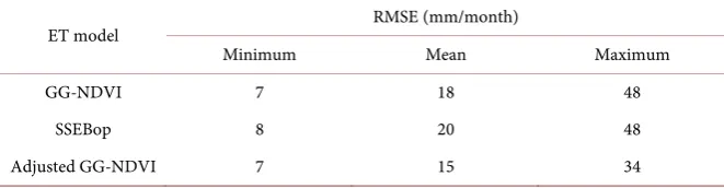
To determine the accuracy of Adjusted GG-NDVI, comparisons were made between the results from the Adjusted GG-NDVI and GG-NDVI and between measured ET data and ET values from SSEBop. These comparisons are shown in Figure 9 and Table 2 across 60 sites. While ET from GG-NDVI at Blodgett in California (Figure 9) showed deviations from measured ET, we can see that the Adjusted GG-NDVI produced ET estimates close to measured ET and reduced mean RMSE from 33 to 22 mm/month for Mize and 17 to 10 mm/month for Blodgett. In Table 2, overall RMSE across 60 sites for GG-NDVI and Adjusted GG-NDVI were found to be 18 mm/month and 15 mm/month, respectively. Figure 10, which presents a histogram of RMSE from the different ET models, shows a significant improvement attributed to the Adjusted GG-NDVI model. With Adjusted GG-NDVI, 38 sites have less than 15 mm/month of RMSE, com-pared to 26 sites with GG-NDVI. These results suggest that the use of the cor-rection function in GG-NDVI can significantly improve accuracy in estimating ET. In addition, Equation (17) can be updated with the new definition of G as

( )

ET+ETP=2f G ETW (19)

where the value of 2f(G) can vary between 1.64 and 3.04 as G varies based on site-specific conditions. The new formulation of the Adjusted GG-NDVI model described in Equation (19) clearly shows that the relationship between ET and ETP is not symmetric with respect to ETW, further confirming the earlier con-clusions that the hypothesis of Bouchet [4] needs to be extended and applied

0 20 40 60

0.00 0.20 0.40 0.60 0.80 1.00 1.20 1.40

R

M

S

E

(

mm/

mo

n

th

)

DOI: 10.4236/nr.2018.94007 103 Natural Resources

Figure 9. Comparison of monthly ET values of GG-NDVI and Adjusted GG-NDVI with measured ET at Boldgett, California from 2000 to 2006.

Figure 10. Comparison of RMSE values between different ET models.

Table 2. Comparison of RMSE between GG-NDVI, SSEBop, and Adjusted GG-NDVI acorss 60 sites.

ET model RMSE (mm/month)

Minimum Mean Maximum

GG-NDVI 7 18 48

SSEBop 8 20 48

Adjusted GG-NDVI 7 15 34

with appropriate corrections.

4. Summary and Conclusions

ET estimation models using the complementary relationship are able to estimate ET in most instances. In particular, the model proposed by Anayah [15] showed excellent performance compared to recently published studies. However, the predictive power of this model and other similar models decreases with increas-ing aridity [9] [12] [15]. In the case of the modified GG model proposed by Anayah [15], a reason may be that relative evaporation in the original GG model was derived using 158 sites in Canada under mostly humid conditions. To over-come this limitation, the previously revised GG model, GG-NDVI (Kim [26]), used the Fu equation to describe relative evaporation on the basis that the Bu-dyko framework can support the complementary relationship [28][29]. The re-sults of GG-NDVI showed improved accuracy compared to other complementary

0 30 60 90 120 150 180 210

2000 2000 2001 2002 2003 2004 2005 2006

E

T

[

mm/

mo

n

th

]

Year

GG-NDVI Observed ET Adjusted GG-NDVI

26 38

0 10 20 30 40 50

0-15 15-30 30-45 45<

N

um

be

r of

s

it

es

RMSE [mm/month]

DOI: 10.4236/nr.2018.94007 104 Natural Resources

relationship models but also showed the need for further refinements, especially under dense vegetation conditions. On the other hand, remote sensing methods are more common as operational models under field conditions. In order to de-termine whether complementary methods such as GG-NDVI can compete and deliver accuracy similar to remote sensing methods, it is important to make ap-propriate comparisons. The objectives of this work were therefore twofold: (1) evaluate the recently developed ET estimation method, GG-NDVI, to see if it could deliver similar accuracy to the commonly used operational remote sensing method, SSEBop and (2) identify the inherent weaknesses of the original com-plementary relationship and make appropriate refinements to further improve the GG-NDVI model, especially under dense vegetation conditions. For this purpose, we selected 60 AmeriFlux sites located across the US.

The first phase of the analysis showed that the GG-NDVI model with the Bu-dyko framework and relative evaporation was found to work reasonably well. Validation with 60 AmeriFlux sites indicated similar levels of accuracy for both SSEBop and GG-NDVI. R-square between GG-NDVI and measured ET ranged from 0.40 to 0.79, overall RMSE of GG-NDVI ranged between 15 and 20 mm/month, and GG-NDVI showed lower RMSE than SSEBop every year. Fur-thermore, the occurrences of RMSE less than 20 mm/month with GG-NDVI were more frequent than SSEBop. Based on these results, we concluded that GG-NDVI is a reliable approach for estimating ET.

The second phase of the analysis showed that the predictive power of GG-NDVI decreased with relative evaporation possibly due to the use of the symmetric complementary relationship in estimating ET. In order to identify the true rela-tionship between ET and ETP with respect to ETW, an exponential correction function was proposed. This phase demonstrated that the inclusion of relative evaporation with a correction function greatly improved the performance of the Adjusted GG-NDVI. For example, 68% of Adjusted GG-NDVI sites had RMSE less than 15 mm/month compared 43% with GG-NDVI.

In essence, this study strengthens the idea that the use of vegetation cover in-formation in the complementary relationship has increased ET estimation pow-er. More importantly, this work showed that the symmetric relationship typically assumed with the complementary relationship may not be valid. Instead, the re-sults show that the symmetrical relationship needs to be updated with a nonli-near correction function as proposed here. A key strength of this study is that the latest proposed version of the GG model, Adjusted GG-NDVI, overcomes limitations of both relative evaporation as proposed by Granger [7] and the as-sumption of a symmetric complementary relationship from the work of Bouchet [4]. Consequently, Adjusted GG-NDVI can lead to significantly increased accu-racy of ET estimates under diverse climate conditions while producing compa-rable or even better results than the SSEBop operational remote sensing model.

References

DOI: 10.4236/nr.2018.94007 105 Natural Resources http://earlywarning.usgs.gov/fews/

[2] Senay, G.B., Bohms, S., Singh, R.K., Gowda, P.H., Velpuri, N.M., Alemu, H. and Verdin, J.P. (2013) Operational Evapotranspiration Mapping Using Remote Sensing and Weather Datasets: A New Parameterization for the SSEB Approach. Journal of the American Water Resources Association, 49, 577-591.

https://doi.org/10.1111/jawr.12057

[3] McMahon, T.A., Finlayson, B.L. and Peel, M.C. (2016) Historical Developments of Models for Estimating Evaporation Using Standard Meteorological Data. WIREs Water, 3, 788-818. https://doi.org/10.1002/wat2.1172

[4] Bouchet, R.J. (1963) Évapotranspiration réelle et potentielle signification climatique.

International Association of Hydrological Sciences, 62, 134-142.

[5] Brutsaert, W. and Stricker, H. (1979) An Advection-Aridity Approach to Estimate Actual Regional Evapotranspiration. Water Resources Research,15, 443-450. https://doi.org/10.1029/WR015i002p00443

[6] Morton, F.I. (1983) Operational Estimates of Areal Evapotranspiration and Their Significance to the Science and Practice of Hydrology. Journal of Hydrology, 66, 1-76. https://doi.org/10.1016/0022-1694(83)90177-4

[7] Granger, R.J. and Gray, D.M. (1989) Evaporation from Natural Nonsaturated Sur-faces.Journal of Hydrology, 111, 21-29.

https://doi.org/10.1016/0022-1694(89)90249-7

[8] Crago, R., Szilagyi, J., Qualls, R.J. and Huntington, J. (2016) Rescaling the Comple-mentary Relationship for Land Surface Evaporation. Water Resources Research, 52, 8461-8471. https://doi.org/10.1002/2016WR019753

[9] Hobbins, M.T., Ramirez, J.A., Brown, T.C. and Classens, L.H.J.M. (2001) The plementary Relationship in Estimation of Regional Evapotranspiration: The Com-plementary Relationship Areal Evapotranspiration and Advection-Aridity Models.

Water Resources Research, 37, 1367-1387. https://doi.org/10.1029/2000WR900358

[10] Kahler, D.M. and Brutsaert, W. (2006) Complementary Relationship between Daily Evaporation in the Environment and Pan Evaporation. Water Resources Research, 42, W05413. https://doi.org/10.1029/2005WR004541

[11] Szilagyi, J. and Jozsa, J. (2008) New Findings about the Complementary Relation-ship Based Evaporation Estimation Methods. Journal of Hydrology,354, 171-186. https://doi.org/10.1016/j.jhydrol.2008.03.008

[12] Xu, C.Y. and Singh, V.P. (2005) Evaluation of Three Complementary Relationship Evapotranspiration Models by Water Balance Approach to Estimate Actual Region-al Evapotranspiration in Different Climate Regions. Journal of Hydrology, 308, 105-121.

[13] Granger, R.J. (1989) A Complementary Relationship Approach for Evaporation from Nonsaturated Surfaces. Journal of Hydrology, 111, 31-38.

https://doi.org/10.1016/0022-1694(89)90250-3

[14] Crago, R. and Crowley, R. (2005) Complementary Relationship for Near-Instantaneous Evaporation. Journal of Hydrology, 300, 199-211.

https://doi.org/10.1016/j.jhydrol.2004.06.002

[15] Anayah, F.M. and Kaluarachchi, J.J. (2014) Improving the Complementary Methods to Estimate Evapotranspiration under Diverse Climatic and Physical Conditions.

DOI: 10.4236/nr.2018.94007 106 Natural Resources [16] Priestley, C.H.B. and Taylor, R.J. (1972) On the Assessment of Surface Heat Fluxes and Evaporation Using Large-Scale Parameters. Monthly Weather Review, 100, 81-92. https://doi.org/10.1175/1520-0493(1972)100<0081:OTAOSH>2.3.CO;2 [17] Penman, H.L. (1948) Natural Evaporation from Open Water, Bare and Grass.

Pro-ceedings of the Royal Society A: Mathematical, Physical and Engineering Sciences, 193, 120-145. https://doi.org/10.1098/rspa.1948.0037

[18] Mu, Q., Zhao, M. and Running, S.W. (2007) Development of a Global Evapotrans-piration Algorithm Based on MODIS and Global Meteorological Data. Remote Sensing of Environment, 111, 519-536. https://doi.org/10.1016/j.rse.2007.04.015 [19] Mu, Q., Zhao, M. and Running, S.W. (2011) Improvements to a MODIS Global

Terrestrial Evapotranspiration Algorithm. Remote Sensing of Environment, 115, 1781-1800. https://doi.org/10.1016/j.rse.2011.02.019

[20] Han, S., Hu, H. and Yang, D. (2011) A Complementary Relationship Evaporation Model Referring to the Granger Model and the Advection-Aridity Mode. Hydro-logical Processes, 25, 2094-2101. https://doi.org/10.1002/hyp.7960

[21] Thompson, S.E., Harman, C.J., Konings, A.G., Sivapalan, M., Neal, A. and Troch, P.A. (2011) Comparative Hydrology across AmeriFlux Sites: The Variable Roles of Climate, Vegetation, and Groundwater. Water Resources Research, 47, W00J07. https://doi.org/10.1029/2010WR009797

[22] Aminzadeh, M., Roderick, M.L. and Or, D. (2016) A Generalized Complementary Relationship between Actual and Potential Evaporation Defined by a Reference Surface Temperature. Water Resources Research, 52, 385-406.

https://doi.org/10.1002/2015WR017969

[23] Venturini, V., Islam, S. and Rodríguez, L. (2008) Estimation of Evaporative Fraction and Evapotranspiration from MODIS Products Using a Complementary Based Model. Remote Sensing of Environment, 112, 132-141.

[24] Venturini, V., Rodriguez, L. and Bisht, G. (2011) A Comparison among Different Modified Priestley and Taylor Equation to Calculate Actual Evapotranspiration with MODIS Data. International Journal of Remote Sensing, 32, 1319-1338. https://doi.org/10.1080/01431160903547965

[25] Szilagyi, J., Crago, R. and Qualls, R.J. (2017) A Calibration-Free Formulation of the Complementary Relationship of Evaporation for Continental-Scale Hydrology.

Journal of Geophysical Research Atmospheres, 122, 264-278. https://doi.org/10.1002/2016JD025611

[26] Kim, H. and Kaluarachchi, J.J. (2017) Estimating Evapotranspiration Using the Complementary Relationship and the Budyko Framework. Journal of Water and Climate Change, 8, 771-790. https://doi.org/10.2166/wcc.2017.148

[27] Li, D., Pan, M., Cong, Z., Zhang, L. and Wood, E. (2013) Vegetation Control on Water and Energy Balance within the Budyko Framework. Water Resources Re-search, 49, 969-976. https://doi.org/10.1002/wrcr.20107

[28] Yang, D., Sun, F., Liu, Z., Cong, Z. and Lei, Z. (2006) Interpreting the Complemen-tary Relationship in Non-Humid Environments Based on the Budyko and Penman Hypotheses. Geophysical Research Letters,33, L18402.

https://doi.org/10.1029/2006GL027657

[29] Zhang, L., Hickel, K., Dawes, W.R., Chiew, F.H.S., Western, A.W. and Briggs, P.R. (2004) A Rational Function Approach for Estimating Mean Annual Evapotranspi-ration. Water Resources Research,40, W02502.

DOI: 10.4236/nr.2018.94007 107 Natural Resources [30] Allam, M.M., Jain Figueroa, A., McLaughlin, D.B. and Eltahir, E.A.B. (2016) Esti-mation of Evaporation over the Upper Blue Nile Basin by Combining Observations from Satellites and River Flow Gauges. Water Resources Research,52, 644-659. https://doi.org/10.1002/2015WR017251

[31] Biggs, T.W., Petropoulos, G.P., Velpuri, N.M., Marshall, M., Glenn, P., Nagler, P. and Messina, A. (2015) Remote Sensing of Actual Evapotranspiration from Crop-lands. CRC Press, Boca Raton.

[32] Su, H., McCabe, M.F., Wood, E.F., Su, Z. and Prueger, J.H. (2005) Modeling Evapo-transpiration during SMACEX: Comparing Two Approaches for Local- and Re-gional-Scale Prediction. Journal of Hydrometeorology, 6, 910-922.

https://doi.org/10.1175/JHM466.1

[33] Bastiaanssen, W.G.M., Menenti, M., Feddes, R.A. and Holtslag, A.A.M. (1998) The Surface Energy Balance Algorithm for Land (SEBAL). 1. Formulation. Journal of Hydrology, 212-213, 198-212. https://doi.org/10.1016/S0022-1694(98)00253-4 [34] Bastiaanssen, W.G.M., Noordman, E.J.M., Pelgrum, H., Davids, G., Thoreson, B.P.

and Allen, R.G. (2005) SEBAL Model with Remotely Sensed Data to Improve Wa-ter-Resources Management under Actual Field Conditions. Journal of Irrigation and Drainage Engineering, 131, 85-93.

https://doi.org/10.1061/(ASCE)0733-9437(2005)131:1(85)

[35] Allen, R.G., Pereira, L.S., Howell, T.A. and Jensen, M.E. (2011) Evapotranspiration Information Reporting: I. Factors Governing Measurement Accuracy. Agricultural Water Management, 98, 899-920. https://doi.org/10.1016/j.agwat.2010.12.015 [36] Senay, G., Budde, M., Verdin, J. and Melesse, A. (2007) A Coupled Remote Sensing

and Simplified Surface Energy Balance Approach to Estimate Actual Evapotranspi-ration from Irrigated Fields. Sensors, 7, 979-1000. https://doi.org/10.3390/s7060979 [37] Senay, G.B., Budde, M.E. and Verdin, J.P. (2011) Enhancing the Simplified Surface

Energy Balance (SSEB) Approach for Estimating Landscape ET: Validation with the METRIC Model. Agricultural Water Management, 98, 606-618.

https://doi.org/10.1016/j.agwat.2010.10.014

[38] Senay, G.B., Leake, S., Nagler, P.L., Artan, G., Dickinson, J., Cordova, J.T. and Glenn, E.P. (2011) Estimating Basin Scale Evapotranspiration (ET) by Water Bal-ance and Remote Sensing Methods. Hydrological Processes, 25, 4037-4049. https://doi.org/10.1002/hyp.8379

[39] Velpuri, N.M., Senay, G.B., Singh, R.K., Bohms, S. and Verdin, J.P. (2013) A Com-prehensive Evaluation of Two MODIS Evapotranspiration Products over the Con-terminous United States: Using Point and Gridded FLUXNET and Water Balance ET. Remote Sensing of Environment, 139, 35-49.

https://doi.org/10.1016/j.rse.2013.07.013

[40] Bastiaanssen, W.G.M., Karimi, P., Rebelo, L.-M., Duan, Z., Senay, G.B., Muttuwatte, L. and Smakhtin, V. (2014) Earth Observation-Based Assessment of the Water Production and Water Consumption of Nile Basin Agro-Ecosystems. Remote Sens-ing, 6, 10306-10334. https://doi.org/10.3390/rs61110306

[41] Allen, R.G., Pereira, L.S., Raes, D. and Smith, M. (1998) Crop Evapotranspira-tion—Guidelines for Computing Crop Water Requirements—FAO Irrigation and Drainage Paper 56. Food and Agriculture Organization of the United Nations, Rome.

[42] Fu, B.P. (1981) On the Calculation of the Evaporation from Land Surface. Chinese Journal of Atmospheric Sciences, 5, 23-31. (In Chinese)

DOI: 10.4236/nr.2018.94007 108 Natural Resources [44] Yang, D., Shao, W., Yeh, P.J.F., Yang, H., Kanae, S. and Oki, T. (2009) Impact of

Vegetation Coverage on Regional Water Balance in the Nonhumid Regions of Chi-na. Water Resources Research, 45, W00A14.

https://doi.org/10.1029/2008WR006948

[45] Allen, R.G., Tasumi, M., Morse, A. and Trezza, R. (2007) Satellite-Based Energy Balance for Mapping Evapotranspiration with Internalized Calibration (METRIC)—Model. Journal of Irrigation and Drainage Engineering, 133, 380-394. https://doi.org/10.1061/(ASCE)0733-9437(2007)133:4(380)

[46] Senay, G.B., Verdin, J.P., Lietzow, R. and Melesse, A.M. (2008) Global Daily Refer-ence Evapotranspiration Modeling and Evaluation. Journal of the American Water Resources Association, 44, 969-979.

https://doi.org/10.1111/j.1752-1688.2008.00195.x

[47] Barrow, C.J. (1992) World Atlas of Desertification. United Nations Environment Programme, Edited by N. Middleton and D. S. G. Thomas, Edward Arnold, Lon-don.

[48] Han, S., Tian, F. and Hu, H. (2014) Positive or Negative Correlation between Actual and Potential Evaporation? Evaluating Using a Nonlinear Complementary Rela-tionship Model. Water Resources Research,50, 1322-1336.

https://doi.org/10.1002/2013WR014151

[49] Roderick, M.L., Hobbins, M.T. and Farquhar, G.D. (2009) Pan Evaporation Trends and the Terrestrial Water Balance. II: Energy Balance and Interpretation. Geogra-phy Compass, 3, 761-780. https://doi.org/10.1111/j.1749-8198.2008.00214.x

[50] Pettorelli, N., Vik, J.O., Mysterud, A., Gaillard, J.M., Tucker, C.J. and Stenseth, N.C. (2005) Using the Satellite-Derived NDVI to Assess Ecological Responses to Envi-ronmental Change. Trends in Ecology and Evolution, 20, 503-510,

https://doi.org/10.1016/j.tree.2005.05.011

[51] Yuan, W.P., Liu, S.G., Yu, G.R., Bonnefond, J.M., Chen, J.Q., Davis, K., Resai, A.R., Goldstein, A.H., Gianelle, D., Rossi, F., Suker, A.E. and Verma, S.B. (2010) Global Estimates of Evapotranspiration and Gross Primary Production Based on MODIS and Global Meteorology Data. Remote Sensing of Environment, 114, 1416-1431. https://doi.org/10.1016/j.rse.2010.01.022

[52] Zhang, S., Yang, H., Yang, D. and Jayawardena, A.W. (2016) Quantifying the Effect of Vegetation Change on the Regional Water Balance within the Budyko Frame-work. Geophysical Research Letters, 43, 1140-1148.

DOI: 10.4236/nr.2018.94007 109 Natural Resources

Abbreviation List

AA: The Advection-Aridity model by [5]

CRAE: The Complementary Relationship Areal Evapotranspiration model by [6] ET: Evapotranspiration

ETP: Potential Evapotranspiration

ETW: Wet Environment Evapotranspiration GG: Granger and Gray Model by [7]

GG-NDVI: The ET model developed by [26]

METRIC: Mapping EvapoTranspiratrion at high Resolution with Internalized Calibration model by [35]

Modified GG: The ET model developed by [15] NDVI: Normalized Difference Vegetation Index NGG: The Normalized GG model by [20]

SEBAL: The Surface Energy Balance Algorithm for Land model by [33] and [34] SSEB: The Simplified Surface Energy Balance model by [36]