© 2019, IRJET | Impact Factor value: 7.211 | ISO 9001:2008 Certified Journal
| Page 851
Music Genre Classification using Machine Learning Algorithms: A
comparison
Snigdha Chillara
1, Kavitha A S
2, Shwetha A Neginhal
3, Shreya Haldia
4, Vidyullatha K S
51,2,3,4,5
Department of Information Science and Engineering,
Dayananda Sagar College of Engineering, Bangalore
– 560078, Karnataka, India
---***---Abstract -
Music plays a very important role in people’slives. Music bring like-minded people together and is the glue that holds communities together. Communities can be recognized by the type of songs that they compose, or even listen to. The purpose of our project and research is to find a better machine learning algorithm than the pre-existing models that predicts the genre of songs. In this project, we built multiple classification models and trained them over the Free Music Archive (FMA) dataset. We have compared the performances of all these models and logged their results in terms of prediction accuracies. Few of these models are trained on the mel-spectrograms of the songs along with their audio features, and few others are trained solely on the spectrograms of the songs. It is found that one of the models, a convolutional neural network, which was given just the spectrograms as the dataset, has given the highest accuracy amongst all other models.
Key Words: Music Information Retrieval, spectrograms,
neural networks, feature extraction, classification
1. INTRODUCTION
Sound is represented in the form of an audio signal having parameters like frequency, decibel, bandwidth etc. A typical audio signal can be expressed as a function of Amplitude and Time. These audio signals come in various different formats which make it possible and easy for the computer to read and analyze them. Some formats are: mp3 format, WMA (Windows Media Audio) format and wav (Waveform Audio File) format.
Companies (such as Soundcloud, Apple Music, Spotify, Wynk etc) use music classification, either to place recommendations to their customers, or simply as a product (like Shazam). To be able to do any of the above two mentioned functions, determining music genres is the first step. To achieve this, we can take the help of Machine Learning algorithms. These machine learning algorithms prove to be very handy in Music Analysis too.
Music Analysis is done based on a song’s digital signatures for some factors, including acoustics, danceability, tempo, energy etc., to determine the kind of songs that a person is interested to listen to.
Music is characterized by giving them categorical labels called genres. These genres are created by humans. A music
genre is segregated by the characteristics which are commonly shared by its members. Typically, these characteristics are related to the rhythmic structure, instrumentation, and the harmonic content of the music. To categorize music files into their respective genres, it is a very challenging task in the area of Music Information Retrieval (MIR), a field concerned with browsing, organizing and searching large music collections.
Classification of genre can be very valuable to explain some interesting problems such as creating song references, tracking down related songs, discovering societies that will like that specific song, sometimes it can also be used for survey purposes.
Automatic musical genre classification can assist humans or even replace them in this process and would be of a very valuable addition to music information retrieval systems. In addition to this, automatic classification of music into genres can provide a framework for development and evaluation of features for any type of content-based analysis of musical signals
The concept of automatic music genre classification has become very popular in recent years as a result of the rapid growth of the digital entertainment industry.
Dividing music into genres is arbitrary, but there are perceptual criteria that are related to instrumentation, structure of the rhythm and texture of the music that can play a role in characterizing particular genre. Until now genre classification for digitally available music has been performed manually. Thus, techniques for automatic genre classification would be a valuable addition to the development of audio information retrieval systems for music.
1.1 Problem Statement
Music plays a very important role in people’s lives. Music bring like-minded people together and is the glue that holds communities together. Communities can be recognized by the type of songs that they compose, or even listen to. Different communities and groups listen to different kinds of music. One main feature that separates one kind of music from another is the genre of the music.
© 2019, IRJET | Impact Factor value: 7.211 | ISO 9001:2008 Certified Journal
| Page 852
1. To build a machine learning model which classifiesmusic into its respective genre.
2. To compare the accuracies of this machine learning model and the pre-existing models, and draw the necessary conclusions.
1.2 Objectives
1. Developing a machine learning model that classifies music into genres shows that there exists a solution which automatically classifies music into its genres based on various different features, instead of manually entering the genre.
2. Another objective is to reach a good accuracy so that the model classifies new music into its genre correctly
3. This model should be better than at least a few pre-existing models.
2. RELATED WORK
Some works published in last two years show that investigations related to musical genre in music information retrieval scenario are not exhausted, and they still remain as an active research topic, as one can note in the following:
I. In Hareesh Bahuleyan, (2018). Music Genre Classification using Machine Learning techniques, the work conducted gives an approach to classify music automatically by providing tags to the songs present in the user’s library. It explores both Neural Network and traditional method of using Machine Learning algorithms and to achieve their goal. The first approach uses Convolutional Neural Network which is trained end to end using the features of Spectrograms (images) of the audio signal. The second approach uses various Machine Learning algorithms like Logistic Regression, Random forest etc, where it uses hand-crafted features from time domain and frequency domain of the audio signal. The manually extracted features like Mel-Frequency Cepstral Coefficients (MFCC), Chroma Features, Spectral Centroid etc are used to classify the music into its genres using ML algorithms like Logistic Regression, Random Forest, Gradient Boosting (XGB), Support Vector Machines (SVM). By comparing the two approaches separately they came to a conclusion that VGG-16 CNN model gave highest accuracy. By constructing ensemble classifier of VGG-16 CNN and XGB the optimised model with 0.894 accuracy was achieved.
II. In Tzanetakis G. et al., (2002). Musical genre classification of audio signals, they have mainly explored about how the automatic classification of audio signals into a hierarchy of musical genres is to be done. They believe that these music genres are categorical labels that are created by humans just to categorise pieces of music. They are categorised by some of the common characteristics. These characteristics are typically related to the instruments that
are used, the rhythmic structures, and mostly the harmonic music content. Genre hierarchies are usually used to structure the very large music collections which is available on web. They have proposed three feature sets: timbral texture, the rhythmic content and the pitch content. The investigation of proposed features in order to analyse the performance and the relative importance was done by training the statistical pattern recognition classifiers by making use of some real-world audio collections. Here, in this paper, both whole file and the real time frame-based classification schemes are described. Using the proposed feature sets, this model can classify almost 61% of ten music genre correctly.
III. In Lu L. et al., (2002). Content analysis for audio classification and segmentation, they have presented their study of segmentation and classification of audio content analysis. Here an audio stream is segmented according to audio type or speaker identity. Their approach is to build a robust model which is capable of classifying and segmenting the given audio signal into speech, music, environment sound and silence. This classification is processed in two major steps, which has made it suitable for various other applications as well. The first step is speech and non- speech discrimination. In here, a novel algorithm which is based on KNN (K- nearest- neighbour) and linear spectral pairs-vector quantization (LSP-VQ) is been developed. The second step is to divide the non-speech class into music, environmental sounds, and silence with a rule- based classification method. Here they have made use of few rare and new features such as noise frame ratio, band periodicity which are not just introduced, but discussed in detail. They have also included and developed a speaker segmentation algorithm. This is unsupervised. It uses a novel scheme based on quasi - GMM and LSP correlation analysis. Without any prior knowledge of anything, the model can support the open-set speaker, online speaker modelling and also the real time segmentation.
IV.
In Tom LH Li et al., (2010). Automatic musicalpattern feature extraction using convolutional
neural network, they made an effort to understand the
© 2019, IRJET | Impact Factor value: 7.211 | ISO 9001:2008 Certified Journal
| Page 853
rate 22050 Hz at 16 bits. The musical patterns wereevaluated using WEKA tool where multiple classification models were considered. The classifier accuracy was 84 % and eventually got higher. In comparison to the MFCC, chroma, temp features, the features extracted by CNN gave good results and was more reliable. The accuracy can still be increased by parallel computing on different combination of genres.
3. DATASET
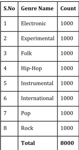
We make use of a subset of the Free Music Archive dataset [FMA paper link], an open and easily accessible database of songs that are helpful in evaluating several tasks in MIR. The subset is called fma_small, a balanced dataset which contains audio from 8000 songs arranged in a hierarchical taxonomy of 8 genres. It provides 30 seconds length of high-quality audio, pre-computed features, together with track-level and user-level metadata, tags and free-form text such as biographies.
The number of audio clips in each category has been tabulated in Table1. Each audio file is about 1 megabyte, hence the entire fma_small dataset is about 8 GB. There are other variants of FMA dataset available too, as shown in Table 2, which are the fma_medium dataset (25,000 tracks of 30s, 16 unbalanced genres (23 GiB)), fma_large dataset (106,574 tracks of 30s, 161 unbalanced genres (98 GiB), fma_full dataset (106,574 tracks of 30s, 161 unbalanced genres (917 GiB)).
The dataset also provides a metadata that allows the users to experiment without dealing with feature extraction. These are all the features the librosa Python library, version 0.5.0 was able to extract. Each feature set (except zero-crossing rate) is computed on windows of 2048 samples spaced by hops of 512 samples. Seven statistics were then computed over all windows: the mean, standard deviation, skew, kurtosis, median, minimum and maximum. Those 518 pre-computed features are distributed in features.csv (present in the fma metadata) for all tracks.
Other datasets that are open source and freely available are shown in the Table 3
4. METHODOLOGY
This section gives the details of data pre-processing followed by a description about the proposed approach to this classification problem.
4.1 Deep Neural Networks
With deep learning algorithms, we can achieve the task of music genre classification without hand-crafted features. Convolutional neural networks (CNNs) prove to be a great choice for classifying images. The 3-channel (R-G-B) matrix of an image is given to a CNN which then trains itself on those images. In this study, the sound wave can be
represented as a spectrogram, which can be treated as an image (Nanni et al., [4]) (Lidy and Schindler, [15]). The task of the CNN is to use the spectrogram to predict the genre label (one of eight classes).
S.No Genre Name Count
1 Electronic 1000
2 Experimental 1000
3 Folk 1000
4 Hip-Hop 1000
5 Instrumental 1000
6 International 1000
7 Pop 1000
8 Rock 1000
[image:3.595.369.505.148.406.2]Total 8000
Table -1: Number of instances in each genre class
dataset clips genres Length [s] Size [
GiB] Size #days
small 8000 8 30 7.4 2.8
medium 25000 16 30 23 8.7
large 106574 161 30 98 37
full 106574 161 278 917 343 Table -2: Variants of FMA dataset
dataset #clips #artists year audio
GTZAN 1000 ~300 2002 yes
MSD 1,000,000 44745 2011 no
AudioSet 2,084,320 - 2017 no
Artist20 1413 20 2007 yes
[image:3.595.307.556.428.747.2]AcousticBrainz 2,524,739 - 2017 no
© 2019, IRJET | Impact Factor value: 7.211 | ISO 9001:2008 Certified Journal
| Page 854
4.1.1 Spectrogram Generation
A spectrogram is a 2D representation of a signal, having time on the x-axis and frequency on the y-axis. In this study, each audio signal was converted into a MEL spectrogram (having MEL frequency bins on the y-axis). The parameters used to generate the power spectrogram using STFT are listed below:
Sampling rate (sr) = 22050
Window size (n_fft) = 2048
Hop length = 512
X_axis: time
Y_axis: MEL
Highest Frequency (f_max) = 8000
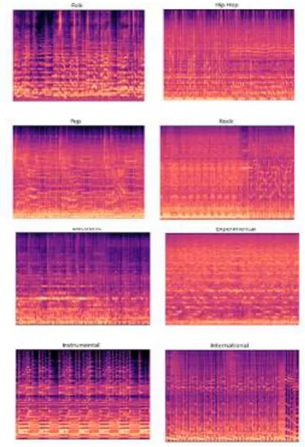
[image:4.595.48.269.302.626.2]The spectrograms from each genre are shown in Figure 1.
Fig- 1: Sample spectrograms for 1 audio track from each music genre
4.1.2 Convolutional Neural Networks
From Figure 2, we can see that there exist some characteristic patterns in the spectrograms of the audio signals belonging to different classes. Hence spectrograms can be considered as ‘images’ and can be given as input to a CNN. A rough framework of the CNN model is shown in Figure 3.
4.1.2.1 Feed Forward Network
[image:4.595.312.557.376.475.2]A CNN is a feed-forward network, that is, input examples are fed to the network and transformed into an output; with supervised learning, the output would be a label, a name applied to the input. That is, they map raw data to categories, recognizing patterns that may signal, for example, that an input image should be labeled “folk” or “experimental”. A feedforward network is trained on labeled images until it minimizes the error it makes when guessing their categories. With the trained set of parameters (or weights, collectively known as a model), the network sallies forth to categorize data it has never seen. A trained feedforward network can be exposed to any random collection of photographs, and the first photograph it is exposed to will not necessarily alter how it classifies the second. Seeing spectrogram of a folk song will not lead the net to perceive a spectrogram of an experimental song next. That is, a feedforward network has no notion of order in time, and the only input it considers is the current example it has been exposed to. Feedforward networks are amnesiacs regarding their recent past; they remember nostalgically only the formative moments of training.
Fig -2: CNN Framework
4.1.2.2 Operations Of CNN
Each block in a CNN consists of the following operations:
Convolution: This step involves a matrix filter (say 3x3 size) that is moved over the input image which is of dimension image width x image height. The filter is first placed on the image matrix and then we compute an element-wise multiplication between the filter and the overlapping portion of the image, followed by a summation to give a feature value.
Pooling: This method is used to reduce the dimension of the feature map obtained from the convolution step. By max pooling with 2x2 window size, we only retain the element with the maximum value among the 4 elements of the feature map that are covered in this window. We move this window across the feature map with a pre-defined stride.© 2019, IRJET | Impact Factor value: 7.211 | ISO 9001:2008 Certified Journal
| Page 855
powerful, we need to introduce some non-linearity. Forthis purpose, we can apply an activation function such as Rectifier Linear Unit (ReLU) on each element of the feature map.
The model consists of 3 convolutional blocks (conv base), followed by a flatten layer which converts a 2D matrix to a 1D array, which is then followed by a fully connected layer, which outputs the probability that a given image belongs to each of the possible classes.
The final layer of the neural network outputs the class probabilities (using the softmax activation function) for each of the eight possible class labels. The cross-entropy loss is computed as shown below:
where, M is the number of classes; yo,c is a binary indicator whose value is 1 if observation o belongs to class c and 0 otherwise; po,c is the model’s predicted probability that observation o belongs to class c. This loss is used to backpropagate the error, compute the gradients and thereby update the weights of the network. This iterative process continues until the loss converges to a minimum value.
4.1.3 Convolutional Recurrent Neural Network
To compare the performance improvement that can be achieved by the CNNs, we train a Convolutional Recurrent Neural Network, which is a combination of convolutional neural networks and recurrent neural networks.
4.1.3.1 Recurrent Neural Networks
Recurrent nets are a type of artificial neural network designed to recognize patterns in sequences of data, such as textual data, genomes, audio, video, or numerical times series data emanating from sensors, stock markets and government agencies. These algorithms take time and sequence into account, they have a temporal dimension. RNNs are applicable even to images, which can be decomposed into a series of patches and treated as a sequence.
Recurrent networks are distinguished from feedforward networks by that feedback loop connected to their past decisions, ingesting their own outputs moment after moment as input. It is often said that recurrent networks have memory. Adding memory to neural networks has a purpose: There is information in the sequence itself, and recurrent nets use it to perform tasks that feedforward networks can’t.
Long Short-Term Memory networks – usually just called “LSTMs” – are a special kind of RNN, capable of learning
long-term dependencies. They were introduced by Hochreiter & Schmidhuber (1997).
4.1.3.2 CRNN Model Details
The CNN-RNN model, shortly called as CRNN model has 3 1-dimensional Convolution Layers followed by an LSTM layer of the RNN, which is then followed by a fully connected dense layer, which is the output layer. The batch size used in this model is 32, number of epochs is maintained as 30, to keep the evaluation and comparison fair. The activation function used is ReLU. To avoid overfitting of the data, Dropout of 0.2 is implemented in the hidden layers.
4.1.4 CNN-RNN Parallel Model
This model runs the CNN model and the RNN model in parallel, keeping all the metrics and regularization factors the same as implemented in the previous models. The idea is to compare a simple CNN model with these robust, complex models to assess the performance metrics and compare the models.
4.1.5 Implementation Details
The spectrogram images have a dimension of 150 x 150. For the feed-forward network connected to the conv base, a 512-unit hidden layer is implemented. Over-fitting is a common issue in neural networks. In order to prevent this, we adopted the following strategy:
Dropout [21]: This is a regularization mechanism in which we shut-off some of the neurons (set their weights to zero) randomly during training. In each iteration, we use a different combination of neurons to predict the final output, thereby randomizing the training cycles. A dropout rate of 0.2 is used, i.e., a given weight is set to zero during an iteration, with a probability of 0.2.
The dataset is randomly split into training set (80%), validation set (10%), testing set (10%). The same split is used for all the comparisons.
The neural networks are implemented in Python using Tensorflow. All models were trained for 30 epochs with a batch size of 64. The optimizer used in these neural networks was the ADAM optimizer. One epoch refers to one iteration over the entire training set.
4.2 Feature Extraction
© 2019, IRJET | Impact Factor value: 7.211 | ISO 9001:2008 Certified Journal
| Page 856
4.2.1 Time Domain Features
These are the features which were extracted from the raw audio signal.
Central moments: This consists of the mean, standard deviation, skewness and kurtosis of the amplitude of the signal.
Zero Crossing Rate (ZCR): This point is where the signal changes sign from positive to negative. The entire 30 second signal is divided into smaller frames, and the number of zero-crossings present in each frame are determined. The average and standard deviation of the ZCR across all frames are chosen as representative features.
Root Mean Square Energy (RMSE): The energy signal in a signal is calculated as
RMSE is calculated frame by frame and then the average and standard deviation across all frames is taken.
Tempo: Tempo refers to the how fast or slow a piece of music is. Tempo is expressed in terms of Beats Per Minute (BPM). We take the aggregate mean of the Tempo as it varies from time to time.
4.2.2 Frequency Domain Features
The audio signal is first transformed into the frequency domain using the Fourier Transform. Then the following features are extracted.
Mel-Frequency Cepstral Coefficients (MFCC): Introduced in the early 1990s by Davis and Mermelstein, MFCCs have been very useful features for tasks such as speech recognition.
Chroma Features: This is a vector which corresponds to the total energy of the signal in each of the 12 pitch classes. (C, C#, D, D#, E ,F, F#, G, G#, A, A#, B). Then the aggregate of the chroma vectors is taken to get the mean and standard deviation.
Spectral Centroid: This corresponds to the frequency around which most of the energy is centered. It is a magnitude weighted frequency calculated as:
where S(k) is the spectral magnitude of frequency bin k and f(k) is the frequency corresponding to bin k.
Spectral Contrast: Each frame is divided into a pre-specified number of frequency bands. And, within each frequency band, the spectral contrast is calculated as the difference between the maximum and minimum magnitudes.
Spectral Roll-off: This feature corresponds to the value of frequency below which 85% of the total energy in the spectrum lies.
For each of the spectral features described above, the mean and standard deviation of the values taken across frames is considered as the representative final feature that is fed to the model.
These definitions are taken from the work of (Hareesh Bahuleyan [3]).
4.3 Classifier
This section provides a brief overview of the machine learning classifier adopted in this study.
Logistic Regression (LR): This linear classifier is generally used for binary classification tasks. For this multi-class classification task, the LR is implemented as a one-vs-rest method. That is, 8 separate binary classifiers are trained. During test time, the class with the highest probability from among the 8 classifiers is chosen as the predicted class.
Simple Artificial Neural Network (ANN): An artificial neuron network (ANN) is a computational model based on the structure and functions of biological neural networks. Information that flows through the network affects the structure of the ANN because a neural network changes - or learns, in a sense - based on that input and output. ANNs are considered nonlinear statistical data modelling tools where the complex relationships between inputs and outputs are modelled or patterns are found. This model takes a csv file of the handcrafted features that are extracted from the audio clips using librosa library and gives an output with the functionality similar to the Logistic Regression logic that is described above.
5. EVALUATION
5.1 Metrics
In order to evaluate the performance of the models, the following metric will be used.
© 2019, IRJET | Impact Factor value: 7.211 | ISO 9001:2008 Certified Journal
| Page 857
5.2 Results and Discussion
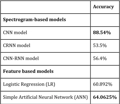
This section discusses the results of various modelling approaches discussed in Section 4 and their accuracies. These accuracies are shown in Table 4.
The best performance in terms of accuracy is observed for the CNN model that uses only the spectrogram as an input to predict the music genre with a test accuracy of 88.54%. The CRNN model and the CNN model, however robust and complex their design is, does not give a good accuracy even though the regularization metrics are modified or the epochs are increased. The reason behind this low test accuracy rate could be the limited dataset of 8000 audio tracks. Increase in the dataset might improve the accuracy of these models.
Accuracy
Spectrogram-based models
CNN model 88.54%
CRNN model 53.5%
CNN-RNN model 56.4%
Feature based models
Logistic Regression (LR) 60.892%
[image:7.595.42.281.276.483.2]Simple Artificial Neural Network (ANN) 64.0625%
Table 4: Accuracies of various models
When the models that use handcrafted features are compared, we can see that LR model and the ANN model give a fairly close test accuracy, even though it is comparatively low when we consider the CNN model’s accuracy. Again, a bigger dataset might give better results.
6. CONCLUSION
In this paper, music genre classification is studied using the Free Music Archive small (fma_small) dataset. We proposed a simple approach to solving the classification problem and we drew comparisons with multiple other complex, robust models. We also compared the models based on the kind of input it was receiving. Two kinds of inputs were given to the models: Spectrogram images for CNN models and audio features stored in a csv for Logistic Regression and ANN model. Simple ANN was determined to be the best feature-based classifier amongst Logistic Regression and ANN models with a test accuracy of 64%. CNN model was determined to be the best spectrogram-based model amongst CNN, CRNN and CNN-RNN parallel models, with an accuracy of 88.5%. CRNN and CNN-RNN models are expected to perform well if the dataset is increased. Overall, image
based classification is seen to be performing better than feature based classification.
ACKNOWLEDGEMENT
We would like to give our heartfelt thanks to our guides Mrs. Latha A P for helping us choose the domain of our project and being a constant support and to Dr Kavitha A S for being encouraging us throughout the journey of this project.
REFERENCES
[1] Michaël Defferrard, Kirell Benzi, Pierre Vandergheynst,
Xavier Bresson. FMA: A Dataset For Music Analysis. Sound; Information Retrieval. arXiv:1612.01840v3, 2017.
[2] Tom LH Li, Antoni B Chan, and A Chun. Automatic musical pattern feature extraction using convolutional neural network. In Proc. Int. Conf. Data Mining and Applications, 2010.
[3] Hareesh Bahuleyan, Music Genre Classification using
Machine Learning Techniques, University of Waterloo, 2018
[4] Loris Nanni, Yandre MG Costa, Alessandra Lumini,Moo Young Kim, and Seung Ryul Baek. Combining visual and acoustic features for music genre classification. Expert Systems with Applications 45:108–117, 2016.
[5] Thomas Lidy and Alexander Schindler. Parallel
convolutional neural networks for music genre and mood classification. MIREX2016, 2016.
[6] Chathuranga, Y. M. ., & Jayaratne, K. L. Automatic Music
Genre Classification of Audio Signals with Machine Learning Approaches. GSTF International Journal of Computing, 3(2), 2013.
[7] Fu, Z., Lu, G., Ting, K. M., & Zhang, D. A survey of audio
based music classification and annotation. IEEE Transactions on Multimedia, 13(2), 303–319, 2011.
[8] Liang, D., Gu, H., & Connor, B. O. Music Genre
Classification with the Million Song Dataset 15-826 Final Report, 2011.
[9] G Tzanetakis and P Cook. Musical genre classification of audio signals. IEEE Trans. on Speech and Audio Processing, 2002.
[10] D PW Ellis. Classifying music audio with timbral and
chroma features. In ISMIR, 2007.
© 2019, IRJET | Impact Factor value: 7.211 | ISO 9001:2008 Certified Journal
| Page 858
[12] T Bertin-Mahieux, D PW Ellis, B Whitman, and P
Lamere. The million song dataset. In ISMIR, 2011.
[13] A Porter, D Bogdanov, R Kaye, R Tsukanov, and X
Serra. Acousticbrainz: a community platform for gathering music information obtained from audio. In ISMIR, 2015.
[14] S. Lippens, J.P Martens, T. De Mulder, G. Tzanetakis.
A Comparison of Human and Automatic Musical Genre Classification. 2004 IEEE International Conference on Acoustics, Speech, and Signal Processing, 2004. 1520-6149, IEEE.
[15] Tao Li and George Tzanetakis, Factors in automatic
musical genre classification, in Proc. Workshop on applications of signal processing to audio and acoustics WASPAA, New Paltz, NY, 2003, IEEE.
[16] Lonce Wyse, Audio Spectrogram representations for
processing with Convolutional Neural Networks, National University of Singapore, 2017.
[17] Michael I. Mandel and Daniel P.W. Ellis, Song-level
Features and Support Vector Machines for Music Classification, Queen Mary, University of London, 2005.
[18] Yibin Zhang and Jie Zhou, Audio Segmentation based
on Multi-Scale Audio Classification, 2004 IEEE International Conference on Acoustics, Speech, and Signal Processing, IEEE, 2004, 1520-6149
[19] Lie Lu, Hong-Jiang Zhang, Hao Jiang, Content Analysis for Audio Classification and Segmentation, Published in: IEEE Transactions on Speech and Audio Processing ( Volume: 10 , Issue: 7 , Oct 2002 ), 1063-6676
[20] Alex Krizhevsky, Ilya Sutskever, Geoffrey E. Hinton,
ImageNet Classification with Deep Convolution Neural Networks, Published in Advances in Neural Information Processing Systems, 2012.
[21] Nitish Srivastava, Geoffrey Hinton, Alex Krizhevsky,