Self-Organising Fuzzy Logic Classifier
Xiaowei Gu1 and Plamen P. Angelov1,2* 1
School of Computing and Communications, Lancaster University, Lancaster, LA1 4WA, UK 2
Technical University, Sofia, 1000, Bulgaria (Honorary Professor) e-mail: {x.gu3, p.angelov}@lancaster.ac.uk
Abstract- In this paper, we present a self-organising nonparametric fuzzy rule-based classifier. The proposed approach identifies prototypes from the observed data through an offline training process and uses them to build a 0-order AnYa type fuzzy rule-based system for classification. Once primed offline, it is able to continuously learn from the streaming data afterwards to follow the changing data pattern by updating the system structure and meta-parameters recursively. The meta-parameters of the proposed approach are derived from data directly. By changing the level of granularity, the proposed approach can make a trade-off between performance and computational efficiency, and, thus, the classifier is able to address a wide variety of problems with specific needs. The classifier also supports different types of distance measures. Numerical examples based on benchmark datasets demonstrate the high performance of the proposed approach and its ability of handling high-dimensional, complex, large-scale problems.
Keywords- classification, fuzzy rule-based systems, self-organising, recursive
1. Introduction
Classification is one of the hotly studied problems in machine learning [24]. Till now, various classification algorithms have been successfully developed and widely used in different areas i.e. remote sensing [46],[47], face recognition [10],[25], handwritten digits recognition [13],[21], etc.
Current classification approaches have different architectures. In general, considering their operating mechanisms, the existing approaches can be categorised into two major types: 1) offline [13],[14],[27] and 2) online [6],[8],[21],[31],[34],[38],[39],[44]. The offline approaches are trained with static datasets and once the training process is finished, the classifiers stop learning and allow no further modification to their structure. The majority of the offline approaches were developed during the time that data was not considered to be in large-scale, streaming and dynamically evolving. Nowadays, as we are living in the era of the so-called “Big Data”, these approaches become less applicable. There are two types of online classification approaches, namely, 1) incremental [31],[34],[44] and 2) evolving [6],[8],[21],[38],[39]. Online approaches can be of “one-pass” type, which means that they are able to consistently learn from newly arrived data samples and only store the key information in memory, meanwhile, discard all the processed training samples. The evolving approaches [6],[8],[21],[38],[39], as the more advanced branch of online approaches, further address the problem of changing data pattern in nonstationary environments by continuously evolving system structure and recursively updating meta-parameters. Compared with the other types, evolving approaches are more memory- and computation- efficient and, thus, are more frequently used in real-world applications. On the other hand, the performance of the online approaches, including the evolving ones, is sensitive to the order of data samples.
Very often in real situations, a part of the data is available in a static form, while the rest is observed sequentially in a streaming form. Offline approaches ignore the fact that the data pattern may change with more data available. However, it is also unnecessary for an approach to learn online from the very beginning of the data stream because initialising the system with the available static data in an offline manner can guarantee a more robust performance.
Furthermore, many existing approaches also rely heavily on 1) prior assumptions, which usually impose models with parameters which depend on the data generation model, i.e. Gaussian distribution [29], and 2) user inputs, which are defined based on prior knowledge of the problem, i.e. radius [15],[21],[50], learning rate [38]/decay rates [39], size of the network [13],[23], etc. In real cases, such prior assumptions are often too strong to be held and user inputs are often hard to define due to the insufficient prior knowledge. In addition, in online scenarios, non-stationary data streams may also invalidate the prior assumptions and user inputs that were established at the initial stage.
[4],[5] and the autonomous data-driven clustering techniques [19]. The SOF classifier has two training stages, 1) offline and 2) online. During the offline stage, it learns from the static data to establish a stable 0-order AnYa type fuzzy rule-based (FRB) system [7]. During the online training stage, the FRB system identified through the offline training process will be updated subsequently with the streaming data to follow the possible drifts and/or shifts in the data pattern. The SOF classifier only keeps the key meta-parameters in memory and is of “one-pass” type during its online training stage; therefore, it is very suitable for large-scale streaming data processing.
Most importantly, the proposed SOF classifier is nonparametric in the sense that no parameters or models are imposed for the data generation model. Employing the EDA quantities as described in section 2.2, the SOF classifier is able to objectively disclose the ensemble properties and mutual distributions of the streaming data based on the empirical observations and all the meta-parameters of the classifier are directly derived from the data without any prior knowledge [4],[5].
The proposed SOF classifier keeps the advantage of objectiveness of the data-driven approaches, and, at the same time, puts users “in the driving seat” by letting users to decide the level of granularity and the type of distance/dissimilarity measure for it. The idea of “granularity” is introduced and defined in [35],[36],[49]. It is well known that a problem can be approached at different levels of specificity (detail) depending on the complexity of the original problem, available computing resources, and particular needs [49]. The level of granularity in the proposed approach is aligned with this concept. However, it has to be stressed that there is no requirement for prior knowledge to decide the level of granularity and it can be given merely based on the preferences of the users. Higher level of granularity leads to a classifier with fine details, and at the same time, results in a risk of overfitting. A lower level of granularity, instead, gives users a classifier trained coarsely but with higher computational efficiency, generalisation and less memory requirement. The SOF classifier is always guaranteed to be meaningful due to its data-driven nature. The choice of the type of distance/dissimilarity measure further gives more freedom to the users and also makes the proposed SOF approach highly adaptive to various applications, e.g. natural language processing. In addition, the SOF classifier can also provide the default level of granularity and distance measure option for the less experienced users.
The remainder of this paper is organised as follows. The theoretical basis of the SOF classifier is summarised in section 2. Section 3 describes the offline training, online training and validation processes of the proposed approach. Section 4 presents how the level of granularity can influence the performance and efficiency of the SOF classifier. Numerical examples serving as a proof of concept are given in section 5, discussions on the convergence and local optimality of the proposed approach are also provided in the same section. Section 6 concludes this paper and gives the direction for future works.
2. Theoretical Basis
In this section, the theoretical basis of the self-organising fuzzy logic (SOF) classifier will be briefly summarised.
2.1. 0-order AnYa Fuzzy Rule-based Systems
AnYa type FRB system was introduced in [7] as an alternative approach to the widely used FRB systems of Takagi-Sugeno [45] or Mamdani [30] types. Comparing with the two predecessors, the antecedent (IF) part of AnYa type fuzzy rules is simplified to a more compact, objective and nonparametric vector form without the need of defining ad hoc membership functions. A 0-order AnYa type fuzzy rule has the following form:
~ 1
~ 2
...
~ N
IF x p OR x p OR OR x p THEN class (1) where x is the input vector; “~” denotes similarity, which can also be seen as a fuzzy degree of satisfaction/membership [7]; pi(
i
1,2,...,
N
) is the ith prototype of the class; Nis the number of prototypes identified from the data samples of this class. For a specific data sample, its label can be decided following different strategies, i.e. “winner-takes-all”, “few-winners-take-all”, “fuzzily weighted average”, etc. In this paper, we use the first one, and the details are given in section 3.3.2.2. Empirical Data Analytics Operators
approach will be described. Their recursive calculation forms for streaming data processing will be given as well.
First of all, let us assume a data set/stream within the real data space
R
M(M is the dimensionality of the space) observed at the Kth time instance denoted by
1, 2,..., K
K
x x x x , where xi xi,1,xi,2,...,xi M, RM , the subscript i denotes the time instance at which the ith data sample, xi arrived. To be more general, we assume that some data samples repeat more than once, namely, xi xj, i j. The set of sorted unique data samples is denoted as
1, 2,...,
K
K U
U
u u u u (ui ui,1,ui,2,...,ui M, ,
K
U K
u x , UK K, UK is the number of unique data samples) and the corresponding repeating times (frequency of occurrence) are
UK
1, 2,..., UK
f f f f (
1 K
U i i
f K
). If no specific declaration is made, all the derivations are conducted at the Kth time instance as a default.1) Cumulative Proximity
Cumulative proximity, introduced earlier [2],[4] is derived empirically from the observed data without prior knowledge or prior assumptions, and can be seen as a square form of the farness. The cumulative proximity of data sample xi is expressed as:
2
1
, ; 1, 2,..., K
K i i j
j
d i K
x x x (2) where d
x xi, j
denotes the distance between xi and xj, which can be any type of distance/dissimilarity measure. It is also worth to be noticed that the average square distance between any two data samples within
x K can be expressed as:
2 1
1 K
K K i
i d
K
x .2) Unimodal Density
Unimodal density, D[4] is used as an indicator of the main data pattern within the EDA framework. The unimodal density at xi is expressed as:
2 1 1 1
2 1
,
; 1, 2,..., 2
2 ,
K K K
l j K l
l j l
K i K
K i
i j j
d
D i K
K
K d
x x x
x
x
x x
(3)
3) Multimodal Density
Multimodal density,
D
MM[4],[5] is estimated at the unique data sample ui as the weighted sum of its unimodal density by its repeating times of occurrence expressed as:
1
; 1, 2,...,2 K
K l
MM l
K i i K i i K
K i
D f D f i U
K
x
u u
u (4) 4) Recursive Calculation Form
The recursive calculation forms of the nonparametric EDA quantities play a significant role in streaming data processing. They ensure the processing techniques to be memory- and computation- efficient. If the Euclidean distance, Mahalanobis distance, the cosine dissimilarity or some other types of distances/dissimilarity are used, one can have elegant recursive calculation forms, with which the EDA quantities can be updated in a more efficient way by keeping only the key meta-parameters in memory. In this paper, we give an example of recursive calculation expressions using Mahalanobis distance. The recursive calculation forms of the EDA quantities with other types of distance metric can be found in the previous works [4],[18].
With Mahalanobis distance used, denoted by
,
1
Ti j i j K i j
d x x x x x x (i j, 1, 2,...,K), the
recursive calculation expression is given as:
1
T 1 T
K i K i K K i K XK K K K
where K is the covariance matrix,
T 1 1 1 KK l K l K
l
K
x
x
; 1 T
1
1 K
K l K l l
X K
x x ;1
1 K
K l
l K
x .
The covariance matrix, K and the global mean, μk can be updated recursively as:
1 1 1
1 1
;
K K K
K
K K
x x
(6)
T T
1 1 1 1
1 1
;
K K K K
K
K K
X X x x X x x (7)
T
1
K K K K
K K
X
(8) The sum of cumulative proximities of all the existing data samples is given as [21]:
2
1 T
21
2 2
K
K l K K K K
l
K X K M
x (9) and, accordingly, the unimodal density at xi is calculated recursively as:
2 1 T
T
T 1
1 1 T
2 1
2
1
K K K K K i
i K K i K i K K i K K K K K
K X D
K K X
M x x x x x
(10)
From the equations (6)-(10) one can see that, if the Mahalanobis distance is used, one can recursively calculate the cumulative proximity and density of new data samples by only keeping μK and XK in the memory.
However, we have to admit that not all kinds of distance/dissimilarity measures support such an elegant form of recursive calculation, and for these types of measure, the following general recursive calculation expressions still hold [2]:
2
1 ,
K i K i d i K
x
x x x (11a)
1
1
1 1
2
K K
K j K j K K
j j
x
x x (11b)
1 1 1 2 1 2 2 , KK j K K
j K i
K i i K
D K d
x xx
x x x (11c) Generally, Euclidean distance is the most widely used distance metric, and its effectiveness and validity as the distance measure, in most cases, are guaranteed. If the data generation model follows a Gaussian distribution or some similar distributions, Mahalanobis distance would be a good choice. While in high dimensional problems, cosine dissimilarity is free from the “curse of dimensionality” and thus, is more effective and more frequently used [1],[9],[42].
On the other hand, we have to stress that the most suitable choice of distance/dissimilarity measure is always problem-specific, and one can use the current knowledge in the problem domain to choose the desired measure for a reasonable approximation and a desired classification result. However, this is out of the range of this paper. In this paper, we only consider the general cases without using prior knowledge.
3. SOF classifier
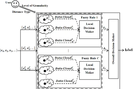
Fig. 1. Architecture of the Self-Organising Fuzzy Logic (SOF) classifier 3.1. Offline Training
The offline training process of the SOF classifier is category-wise as shown in Fig. 1, the classifier will identify prototypes from each class separately and form a 0-order AnYa type fuzzy rule based on the identified prototypes per class (in the form of equation (1)). The training processes of the fuzzy rules of different classes will not influence each other. In the rest of this subsection, we assume that the training process is conducted on data samples of the cth class (
c
1,2,
,
C
) denoted by
c
1, 2,..., c
c c c c
K
K
x x x x (
c
c
K K
x x ), and the corresponding unique data sample set and frequencies of occurrence are denoted, respectively, by
c
1, 2,..., c
K Kc c c c
U U
u u u u and
c
1 , 2,..., c
K Kc c c c
U U
f f f f , where
K
c is the number of data samples with
cc K x , c
K
U is the number of unique data samples of the cth class. Considering all the classes, we have
1
C c c
K K
and1
C c K K c
U U
.In the proposed approach, prototypes are identified based on the densities and the mutual distributions of
the data samples. Firstly, multimodal densities
21 1 2 1
,
2 ,
c c
c c
K K
c c l j l j
MM c c i i
K K
c c c
i j j
d
D f
K d
x x u
u x
(i1, 2,..,UKc) [4],[5] at all
the unique data samples within
c Kc
U
u are calculated using equation (4). Then, the data samples are ranked in a list denoted by
r in terms of their mutual distances and values of multimodal density.By finding out the data sample with the highest multimodal density, 1
1,2,...,
arg max c c K
MM c i K i U
D
r u , the first
minimum distance to r1: 2
1
1,2,..., 1 arg min c K c i i U d r r ,u . The third element of
r denoted by r3 is identified based on the minimum distance to r2. By repeating the process and until all the data samples have been selected, the full list
r is built and the multimodal densities of
cK
c
U
u are ranked accordingly with the list, denoted by
c
MM K
D r [19]. It needs to be stressed that once a data sample is selected into
r , it cannot be selected for a second time.Prototypes, denoted by
0
p , are then identified as the local maxima of the ranked multimodal densities,
c
MM
K
D r using Condition 1 [19]:
Condition 1:
1
1
0
c c c c
MM MM MM MM
i i i i i
K K K K
IF D r D r AND D r D r THEN r p (12) Once all the prototypes are identified using equation (12), one may notice some less representative ones within
0
p , therefore, it is necessary to conduct a filtering operation to remove them from
0
p .
Before the filtering operation starts, we firstly use the prototypes to attract nearby data samples to form data clouds [7] resembling Voronoi tessellation [32]:
0
arg min , ; c
c
i i K
winning prototype d
p p
x p x x (13) After all the data clouds are formed around the existing prototypes
0
p , one can obtain the centres of the data clouds denoted by
0
and the multimodal densities at the centres are calculated using equation (4) as
c c
MM
i i i
K K
D
S D
, where
0
i
; Si is the support (number of members) of the ith data cloud. Then, for each data cloud, assuming the ith one (
0
i
), the collection of the centres of its neighbouring data clouds, denoted by
neighbi ouring
are identified using the following principle:
Condition 2:
2
,
, c c L i neighbour i ng
j K j
i
IF d G THEN (14)
where
0,
j j i
; ,
c
c L K
G is defined as the average radius of local influential area around each data sample, which is corresponding to the Lth (
L
1, 2,3,...
) level of granularity and is derived from the data of the cth class based on the users’ choice in an offline way. Section 4 will explain how to derive ,cL c K
G in detail. Finally, the most representative prototypes of the cth class, denoted by
p c, are selected out from the centres of the existing data clouds satisfying Condition 3 [19]:Condition 3:
maxneighbour
c c in i g c MM MM i i K K
IF D D THEN
p (15)After all the representative prototypes of the cth class
p care identified, one can build the AnYa type fuzzy rule in the following form, where Ncis the number of prototypes in
p c.
~ 1
~ 2
...
~ c
c c c
N
IF x p OR x p OR OR x p THEN class c (16) The main procedure of the offline training process of the proposed SOF classifier is summarised in in the following pseudo code.
Offline training process of the SOF classifier
i. Calculate MM
D at
c Kc
U
u ; ii. Find 1
1,2,...,
arg max c c K MM c i K i U D
r u and exclude r1 from
cK
c
U
u ; iii. 1;
1;
c
c
1 ;MM MM
K K
iv. While c 0 K U k * k k 1; * Find
1
arg min
c c
c i UK
c k d k i
u u
r r ,u and exclude rk from
c Kc
U
u ;
*
;
c
c
c
;MM MM MM
k DK DK DK k
r r r r r r
v. End While vi. Identify
0
p using Condition 1; vii. Form data clouds around
0
p ; viii. Identify
0
from the data clouds; ix. Calculate MMD at
0
;
x. Identify
neighbouring using Condition 2; xi. Identify
p c using Condition 3; xii. Create the cth fuzzy rule with
p c. 3.2. Online Self-Evolving TrainingDuring the online training stage, the SOF classifier continues to update its system parameters and structure with the streaming data on a sample-by-sample basis. Furthermore, because the EDA quantities employed by the SOF classifier can be updated recursively, it can be of “one-pass” type, and its computation- and memory-efficiency is also guaranteed. In this subsection, we assume that the training process of the SOF classifier with the static dataset
K
x has been finished and new data samples start to arrive in a data stream form. Similar to the offline training stage, during the online training stage, the fuzzy rules of different classes are updated separately. During the online stage, recursive calculation expressions of the EDA quantities with Mahalanobis distance are used. Nonetheless, we want to stress again that the proposed approach can use various types of distance/dissimilarity measures (see subsection 2.2).
Assuming at K+1th instance, a new data sample of the cth class, denoted as
1 c
c K
x , arrives, the SOF classifier, firstly, updates the meta-parameters c
c K
, cc K
X , c
c K
to
1 c c K
, 1 c c K X , 1 c c K using equations (6)-(8). The average radius of local areas of influence, ,c
L c K
G is updated afterwards in a recursive way based on the ratio between c
c K
d and ,c
L c K G :
1 2 1 1, 1 , ,
1 2 1 1 1 1 c c c
c c c c
c c K c l K c c l
c L K c L c L
c
K K K K
c K l K c l K d
G G G
d K
x x (17)where c
c K d and
1 c
c K
d denote the average square distances between any two data samples within
cc K x and
c 1c K
x , respectively.
As a special case, for Mahalanobis distance (equation (9)), , ,
1 c c L c c K K L
G G . As we can see from equation (17), instead of deriving ,
1 c
K L c
G in an offline way, which will be described in section 4 in detail, equation (17) largely reduces the computational complexity and memory requirement, and further largely improves the efficiency of the SOF classifier.
Then,
1 c
c K
Condition 4:
1 1 1 1 1 1
1
max min
c c c c c c
c c
c
c c
K K K K K K
c c
K
IF D D OR D D
THEN p p p p
x p x p
x p
(18)
where equation (10) is used for calculating
1 1
c c
c
K K
D x and
1 c
K
D p (p
p c). If1 c
c K
x meets Condition 4, a new prototype is added to the fuzzy rule of the cth class (equation (16)) and the meta-parameters of the SOF classifier are updated as follows:
1
1; c c ; c 1; c
c c
c c c c c c
N K N N
N N p x S p p p (19) If Condition 4 is unsatisfied, we still need to check whether
1 c
c K
x is very close to an existing prototype by using Condition 5 [19].
Condition 5:
2 ,
1 1 1
minc c , c c
c
c c L c
K K K
IF d G THEN
p p
x p x p (20) If Condition 5 is met, a new prototype is added to the fuzzy rule of the cth class (
cc c c
N
p p p ) and
the corresponding new data cloud with meta-parameters initialised by equation (19) is added to the SOF classifier.
If Conditions 4 and 5 are both unsatisfied,
1 c
c K
x is assigned to the nearest prototype
* arg minc c 1,
c c
n d K
p p
p x p and the meta-parameters of the corresponding data cloud are updated as follows [2]:
*
* * 1 * *
* *
1
; 1
1 1 c
c
c n c c c c
n c n c K n n
n n
S
S S
S S
p p x (21) After the meta-parameters of the classifier are updated, the AnYa type fuzzy rule (equation (16)) will be updated accordingly and the SOF classifier is ready for processing the next data sample or conducting classification.
The main procedure of the online training process of the proposed SOF classifier is summarised in the following pseudo code.
Online training process of the SOF classifier While a new data sample of the cth class
1 c
c K
x is available (or until interrupted) i. Update c
c K
, cc K
X , c
c K
, ,c
L c K G to 1 c c K
, 1 c c K X , 1 c c K , , 1 c K L c G ; ii. Calculate D at1 c
c K
x and
p c;iii. If (Condition 4 is met) Or (Condition 5 is met) Then
* 1; c c 1; c 1;
cc c
c c c c c c
N K N N
N N p x S p p p
iv. Else * Find c*
n p ;
* *
* * 1 * *
* *
1
; 1
1 1 c
c
c n c c c c
n c n c K n n
n n
S
S S
S S
p p x ;
v. End If vi. KcKc1;
vii. Update the fuzzy rule; End While
3.3. Validation
[image:8.595.68.528.474.668.2]
2 ,
max ; 1, 2,...,
c
d
c e c C
x p
p p
x (22) Based on the C firing strengths of the C fuzzy rules correspondingly (one per rule), the label of x is decided by the overall decision-maker using the “winner-takes-all” principle as follows:
1,2,...,arg max c
c C
label
x (23)
4. Classification under Different Levels of Granularity
Since the SOF classifier is a prototype-based approach, it is of paramount importance to define a suitable local area of influence for each prototype in order to increase the descriptive ability of the fuzzy rules and at the same time, avoid overlap. There are two commonly adopted ways to define this. The first one is to define a radius based on prior knowledge [15]. The second one is to derive it from data following hard-coded principles [29],[38]. However, in most cases, prior knowledge is unavailable, while the hard-coded principles are too sensitive to the nature of the data. The performance of the two approaches is often not guaranteed. In the following part of this section, we will demonstrate how to define the local areas around prototypes based on the data and the level of granularity.
Under the 1st level of granularity (L=1), the average radius of local influential area around each prototype of the cth class, denoted by ,1
c
c K
G , is defined as follows:
2
2 , , , , ,1 ,1 , c c c c K K c c d d c c K K d G Q
x y x x y x y
x y
(24)
where ,1c
c K
Q is the number of the pairs of data samples within
cc K
x between which the distance is smaller than the average distance, c
c K d .
From level 2 to an arbitrary level of granularity (
L
2,3,...,
), one can calculate the average radius iteratively using the following equation:
2 , 1
2 , , , ,
,
,
,
c c L
c c K K c c d G c L c L K K d G Q
x y x x y x y
x y
(25) where ,c 1
c L K
G is the average radius corresponding to (L-1)th level of granularity; ,c
c L K
Q is the number of the pairs of data samples between which the distance is smaller than ,c 1
c L K G .
Compared with the traditional approaches, there are strong advantages in deriving local information in this way. Firstly, ,
c
L c K
G is guaranteed to be valid all the time. Defining the threshold or hard-coded mathematical principles in advance may suffer from various problems, which have been discussed at the beginning of this section. While ,c
L c K
G is derived from the data directly and is always meaningful. There is no need for prior knowledge of data sets/streams, and the level of granularity used by the SOF classifier can be decided merely based on the preferences of the users. Moreover, users are allowed to have freedom to make choices, but at the same time, are not overloaded. Finally, one can always adapt the classifier by changing the level of granularity based on the specific needs. Some problems rely heavily on fine details, while others may need generality only.
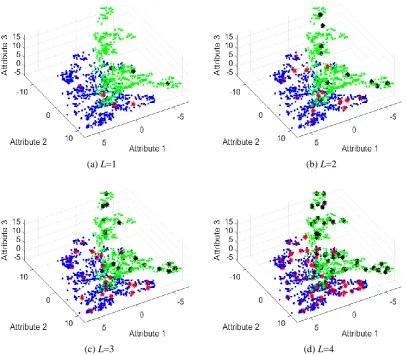
In general, the higher level of granularity is chosen, the more fine details (more prototypes) the SOF classifier extracts from the data, and the classifier achieves a higher performance. At the same time, the SOF classifier may consume more computational and memory resources, and overfitting may also appear. On the contrary, with low level of granularity, the SOF classifier only learns the coarse information from training. Although, the classifier will be more computationally efficient, its performance may be influenced due to the loss of fine information from the data. An illustrative example based on the UCI benchmark dataset named Banknote Authentication1 is given in Fig. 2 with different levels of granularity. In this visual example, the SOF classifier is trained offline using Mahalanobis distance.
(a) L=1 (b) L=2
[image:10.595.75.482.99.454.2](c) L=3 (d) L=4
Fig. 2. Prototypes identified under different levels of granularity based on Banknote Authentication dataset (dots and asterisks in different colours denote data samples and prototypes of different classes). 5. Numerical Examples and Discussions
In this section, numerical examples are provided as a proof of concept. The experiments are conducted using MATLAB R2017a on a PC within Windows 10 operating system, 3.6 GHz dual core Intel 7 processor and 16 GB RAM. The links to the source codes (MATLAB and Python versions) of the proposed approach can be found at: http://www.empiricaldataanalytics.org/downloads.html.
We, firstly, consider the following challenging UCI benchmark datasets for evaluating the performance the SOF classifier:
1) Occupancy detection dataset2;
2) Optical recognition of handwritten digits dataset3; 3) Multiple features dataset4, and
4) Letter recognition dataset5.
The details of the four benchmark datasets are tabulated in Table 1. The occupancy detection dataset contains one training set with 8143 data samples and two testing sets with 2665 and 9752 data samples in each, respectively. In this paper, we combine the two testing sets into one for clarity, and the time stamp of this dataset has been removed. The optical recognition dataset consists of one training set with 3823 data samples and one testing set with 1797 data samples.
2 available at: https://archive.ics.uci.edu/ml/datasets/Occupancy+Detection+ 3
available at: https://archive.ics.uci.edu/ml/datasets/Optical+Recognition+of+Handwritten+Digits
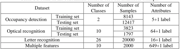
Table 1 Details of the benchmark datasets used for numerical example
Dataset Number of
Classes
Number of Samples
Number of Attributes
Occupancy detection Training set 2 8143 5+1 label
Testing set 12417
Optical recognition Training set 10 3823 64+1 label
Testing set 1797
Letter recognition 26 20000 16+1 label
Multiple features 10 2000 649+1 label
Firstly, the influence of different levels of granularity on the classification results of the proposed SOF approach is studied, and the occupancy detection and optical recognition datasets are used in this experiment. In this example, we consider the offline scenario only and vary the level of granularity, L from 1 to 12. The classification results are tabulated in Table 2 and the performance is measured in terms of classification accuracy, denoted by Acc, the number of identified prototypes, denoted by N(
1
C c c
N N
) and the training time consumption in seconds, denoted by t. Here, the Mahalanobis distance, Euclidean distance and cosine dissimilarity are used. However, for the optical recognition dataset, as the co-variance matrix of the data is not always positive definite, we consider the results obtained using the Euclidean distance and cosine dissimilarity only. The results tabulated are the average of 10 Monte Carlo experiments by randomly descrambling the order of the training samples.From Table 2 one can see that, in general, the higher level of granularity is chosen, the higher accuracy the SOF classifier can exhibit during classification, but the more prototypes the classifier identifies, which can lower down the computation- and memory-efficiency. It is worth to notice that the proposed approach produced the same result in 10 Monte Carlo experiments, which demonstrates that the SOF classifier is invariant to the changes in the order of data samples during the offline training.
One may also notice from Table 2 that the type of distance/dissimilarity measure used also influences the performance of the proposed approach. As the proposed approach accommodates various types of distance/dissimilarity measures, one can use the current knowledge of the problem domain to choose the appropriate distance measure.
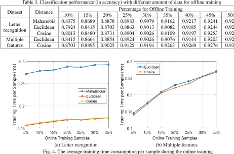
Secondly, the classification performance of the proposed SOF classifier with different amounts of offline training samples is investigated. In this example, we use the letter recognition and multiple features datasets. As the two datasets are both highly complex, we choose the 12th level of granularity to ensure the SOF classifier can learn sufficient details. The percentage of offline training samples is changed from 10% to 50% and the classification is conducted on the remaining 50% of the data in an offline scenario. The results are tabulated in Table 3, which are the averages of 10 Monte Carlo experiments by randomly selecting the training set and testing set. The corresponding average training time consumption (in seconds) is depicted in Fig. 3.
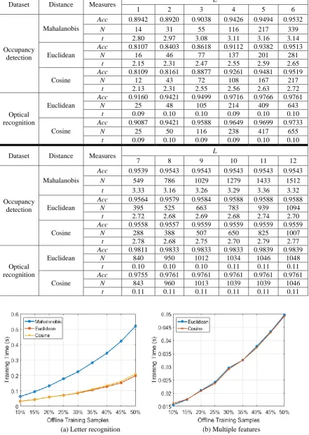
In order to investigate the performance of the proposed approach in an online scenario, we conduct an extra experiment on the two datasets. The SOF classifier is firstly trained with 15% of the data samples in an offline scenario, and then, is trained in an online scenario by using different amounts (from 5% to 35%) of data samples on a sample-by-sample basis. The classification accuracy of SOF classifier is evaluated on the remaining 50% of data samples. The average performance is tabulated in Table 4 after 10 Monte Carlo experiments by randomly selecting the offline training set, online training set and testing set. The corresponding average time consumption per data sample (in milliseconds) during the online training process is given in Fig. 4. In both Tables 3 and 4, the classification results on the multiple feature dataset using the Mahalanobis distance is not given for the same reason mentioned before.
saves the computational resources. Fig. 4 demonstrates the very high computational efficiency (less than 0.3 millisecond per data sample) for the SOF classifier to self-evolve recursively on a sample-by-sample basis.
Table 2 Influence of granularity on classification performance
Dataset Distance Measures L
1 2 3 4 5 6
Occupancy detection
Mahalanobis
Acc 0.8942 0.8920 0.9038 0.9426 0.9494 0.9532
N 14 31 55 116 217 339
t 2.80 2.97 3.08 3.11 3.16 3.14
Euclidean
Acc 0.8107 0.8403 0.8618 0.9112 0.9382 0.9513
N 16 46 77 137 201 281
t 2.15 2.31 2.47 2.55 2.59 2.65
Cosine
Acc 0.8109 0.8161 0.8877 0.9261 0.9481 0.9519
N 12 43 72 108 167 217
t 2.13 2.31 2.55 2.56 2.63 2.72
Optical recognition
Euclidean
Acc 0.9160 0.9421 0.9499 0.9716 0.9766 0.9761
N 25 48 105 214 409 643
t 0.09 0.10 0.10 0.09 0.10 0.10
Cosine
Acc 0.9087 0.9421 0.9588 0.9649 0.9699 0.9733
N 25 50 116 238 417 655
t 0.09 0.10 0.09 0.09 0.10 0.10
Dataset Distance Measures L
7 8 9 10 11 12
Occupancy detection
Mahalanobis
Acc 0.9539 0.9543 0.9543 0.9543 0.9543 0.9543
N 549 786 1029 1279 1433 1512
t 3.33 3.16 3.26 3.29 3.36 3.32
Euclidean
Acc 0.9564 0.9579 0.9584 0.9588 0.9588 0.9588
N 395 525 663 783 939 1094
t 2.72 2.68 2.69 2.68 2.74 2.70
Cosine
Acc 0.9558 0.9557 0.9559 0.9559 0.9559 0.9559
N 288 388 507 650 825 1007
t 2.78 2.68 2.75 2.70 2.79 2.77
Optical recognition
Euclidean
Acc 0.9811 0.9833 0.9833 0.9833 0.9839 0.9839
N 840 950 1012 1034 1046 1048
t 0.10 0.10 0.10 0.11 0.11 0.11
Cosine
Acc 0.9755 0.9761 0.9761 0.9761 0.9761 0.9761
N 843 960 1013 1039 1039 1046
t 0.11 0.11 0.11 0.11 0.11 0.11
[image:12.595.78.520.133.756.2]
(a) Letter recognition (b) Multiple features
Table 3. Classification performance (in accuracy) with different amount of data for offline training
Dataset Distance Percentage for Offline Training
10% 15% 20% 25% 30% 35% 40% 45% 50%
Letter recognition
Mahanobis 0.8375 0.8689 0.8878 0.8983 0.9079 0.9162 0.9217 0.9241 0.9265 Euclidean 0.7924 0.8415 0.8703 0.8863 0.9013 0.9082 0.9185 0.9244 0.9298 Cosine 0.8013 0.8480 0.8731 0.8904 0.9026 0.9109 0.9197 0.9253 0.9296 Multiple
features
Euclidean 0.8415 0.8664 0.8854 0.8924 0.9026 0.9076 0.9144 0.9203 0.9267 Cosine 0.8703 0.8895 0.9025 0.9125 0.9194 0.9263 0.9269 0.9276 0.9366
[image:13.595.93.499.435.520.2]
(a) Letter recognition (b) Multiple features Fig. 4. The average training time consumption per sample during the online training
Table 4. Classification performance (accuracy) with different amount of data for online training following the offline training with 15% of the data
Dataset Distance Percentage for Online Training
5% 10% 15% 20% 25% 30% 35%
Letter recognition
Mahanobis 0.8594 0.8836 0.9012 0.9125 0.9199 0.9279 0.9327 Euclidean 0.8738 0.8910 0.9062 0.9162 0.9231 0.9303 0.9352 Cosine 0.8758 0.8931 0.9070 0.9158 0.9233 0.9293 0.9350 Multiple
features
Euclidean 0.8827 0.9097 0.9166 0.9205 0.9272 0.9340 0.9352 Cosine 0.9062 0.9258 0.9335 0.9316 0.9318 0.9399 0.9409
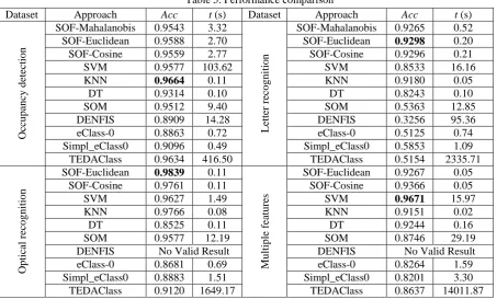
To further evaluate the performance of the SOF classifier with L12, we compare it with a number of “state-of-the-art” approaches in an offline scenario on the four benchmark datasets tabulated in Table 1:
1) Support vector machine (SVM) classifier [14]; 2) K-nearest neighbour (KNN) classifier [16]; 3) Decision tree (DT) classifier [40];
4) Self-organising map (SOM) classifier [37]; 6) DENFIS classifier [22];
7) eClass-0 classifier [8], and 8) TEDAClass classifier [21].
From Table 5 one can see that, the proposed SOF classifier can exhibit very high performance on the four benchmark problems with a very short training process.
Table 5. Performance comparison
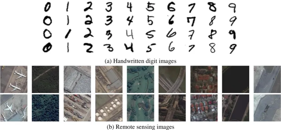
In order to see the performance of the proposed SOF classifier on high-dimensional, complex problems, we further involve the following two benchmark image classification problems:
1) MNIST dataset6, and 2) Singapore dataset7.
MNIST dataset is a large-scale image set for hand-written digits recognition (from “0” to “9”). The training set contains 60000 images and the testing set contains 10000 images (with image size of 28 28 pixels). We use the GIST feature descriptor [33] to extract 1 512 dimensional feature vectors from the central area ( 22 22 pixels) of handwritten digit images [3]. Singapore dataset was constructed from a large high-resolution satellite image of Singapore. This dataset consists of 1086 remote sensing scene images (with original size of 256 256 pixels) of nine classes (“airplane”, “forest”, “harbour”, “industry”, “meadow”, “overpass”, “residential”, “river” and “runway”). We use the 1 4096 dimensional activations of the pre-trained VGG-VD-16 convolution neural network [43] from the first fully connected layer [47] as the feature vectors of the images. The details of two large-scale benchmark problems are tabulated in Table 6. Examples of the images of both datasets are given in Fig. 5. In the following examples, the SOF classifier only uses the Euclidean distance and the cosine dissimilarity, and the 12th level of granularity (L12) for both problems.
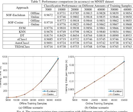
For the MNIST dataset, the SOF classifier is trained in an offline scenario using the training sets with different sizes (5000, 10000, 20000, 30000, 40000, 50000 and 60000 images), and then, is tested on the testing set, and the classification results are tabulated in Table 7. Experiments in the online scenario are also conducted by firstly training the SOF classifier with 5000 images in an offline scenario, and then continuing the training in an online self-evolving manner; the performance with different amounts of training images is tabulated in Table 7 as well. All the results reported in Table 7 are average results of 10 Monte Carlo experiments. The average time consumption of the proposed approach is given in Fig. 6. For the offline scenario, we report the overall time consumption; for the online scenario, we report the time consumption for the SOF classifier to process each image. We also involve the following approaches in the comparison:
1) Support vector machine (SVM) classifier;
6 available at: http://yann.lecun.com/exdb/mnist/
7 available at: http://icn.bjtu.edu.cn/Visint/resources/Scenesig.aspx
Dataset Approach Acc t (s) Dataset Approach Acc t (s)
Occ
u
p
an
cy
d
etec
tio
n
SOF-Mahalanobis 0.9543 3.32
L
etter
r
ec
o
g
n
itio
n
SOF-Mahalanobis 0.9265 0.52
SOF-Euclidean 0.9588 2.70 SOF-Euclidean 0.9298 0.20
SOF-Cosine 0.9559 2.77 SOF-Cosine 0.9296 0.21
SVM 0.9577 103.62 SVM 0.8533 16.16
KNN 0.9664 0.11 KNN 0.9180 0.05
DT 0.9314 0.10 DT 0.8243 0.10
SOM 0.9512 9.40 SOM 0.5363 12.85
DENFIS 0.8909 14.28 DENFIS 0.3256 95.36
eClass-0 0.8863 0.72 eClass-0 0.5125 0.74
Simpl_eClass0 0.9096 0.49 Simpl_eClass0 0.5853 1.09
TEDAClass 0.9634 416.50 TEDAClass 0.5154 2335.71
Op
tical
rec
o
g
n
itio
n
SOF-Euclidean 0.9839 0.11
Mu
ltip
le
fea
tu
res
SOF-Euclidean 0.9267 0.05
SOF-Cosine 0.9761 0.11 SOF-Cosine 0.9366 0.05
SVM 0.9627 1.49 SVM 0.9671 15.97
KNN 0.9766 0.08 KNN 0.9151 0.02
DT 0.8525 0.11 DT 0.9244 0.16
SOM 0.9577 12.19 SOM 0.8746 29.19
DENFIS No Valid Result DENFIS No Valid Result
eClass-0 0.8681 0.69 eClass-0 0.8264 1.59
Simpl_eClass0 0.8883 1.51 Simpl_eClass0 0.8201 3.30
2) K-nearest neighbour (KNN) classifier; 3) Decision tree (DT) classifier;
4) eClass-1 classifier [8]; 5) AutoClass-1 classifier [6] and 6) TEDAClass classifier.
For Singapore dataset, we follow the commonly used experimental protocol [17] by randomly selecting 20% of the images of each class for training and using the rest for testing in an offline scenario. The average classification accuracy is reported in Table 8 after 10 Monte Carlo experiments, where the best result is bolded. We also involve the following “state-of-the-art” approaches in the area of remote sensing for comparison:
1) Spatial pyramid matching kernel (SPMK) [26]; 2) Pyramid of spatial relations (PSR) [11]; 3) Bag-of-visual-words (BoVW) [48];
4) SIFT-based features with sparse coding(SIFTSC) [12];
5) Two-level feature representation with sparse coding (TLFRSC) [17]; 6) Vector of locally aggregated descriptors (VLAD) [20], and
[image:15.595.140.456.309.372.2]7) Two-level feature representation with selection-constrained coding (TLFRSCC) [17]. Table 6 Details of the datasets used for numerical example
Dataset Number of
Classes
Number of Samples
Number of Attributes
MNIST Training set 10 60000 512+1 label
Testing set 10000
Singapore 9 1086 4096+1 label
From Tables 7 and 8 we can see that the proposed SOF classifier can exhibit very high performance compared with the “state-of-the-art” approaches in large-scale, high-dimensional problems.
Fig. 6 shows the high efficiency of the proposed approach in both offline and online training. In addition, one may notice that, in offline scenario, the SOF classifier can be trained on 60000 images for less than 20 minutes, 2 minutes per rule, which is far more efficient than the deep learning-based approaches [13], which require several hours plus several GPUs. In the online scenario, the SOF classifier only needs less than 0.025 second to process each image and is self-evolving.
(a) Handwritten digit images
[image:15.595.72.523.491.699.2](b) Remote sensing images
Fig. 5. Example images of the two benchmark datasets.
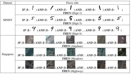
the SOF classifier. Illustrative examples of the fuzzy rules generated from the two benchmark problems are given in Table 9. For visual clarity, we resized the images in the table.
[image:16.595.77.506.139.501.2]From the above numerical examples, one can conclude that the proposed SOF classifier in this paper is a powerful alternative to the existing approaches with high accuracy, transparency and fast self-evolving learning.
Table 7. Performance comparison (in accuracy) on MNSIT dataset
Approach Classification Performance on Different Amounts of Training Samples 5000 10000 20000 30000 40000 50000 60000 SOF-Euclidean Offline 0.9672 0.9731 0.9785 0.9813 0.9828 0.9839 0.9854 Online 0.9746 0.9802 0.9818 0.9835 0.9846 0.9850 SOF-Cosine Offline 0.9718 0.9773 0.9818 0.9844 0.9851 0.9862 0.9855 Online 0.9776 0.9825 0.9845 0.9862 0.9867 0.9868
SVM 0.9776 0.9810 0.9838 0.9856 0.9861 0.9866 0.9869
KNN 0.9678 0.9749 0.9798 0.9824 0.9840 0.9854 0.9861
DT 0.8174 0.8429 0.8654 0.8764 0.8818 0.8890 0.8933
eClass1 0.9685 0.9719 0.9732 0.9746 0.9745 0.9746 0.9746 AutoClass1 0.9691 0.9724 0.9738 0.9744 0.9742 0.9738 0.9742 TEDAClass 0.9716 0.9738 0.9753 0.9768 0.9766 0.9765 0.9763
(a) Offline scenario (b) Online scenario
[image:16.595.174.420.638.739.2]Fig. 6. The average training time consumption with different amounts of training samples On the other hand, we have to admit that the proposed approach does not converge to a locally optimal solution of the problem after the training process. In order to achieve the local optimality, one needs to predefine an objective function and involve an iterative process to minimise the objective function [41]. Because of the greedy type search used in the SOF classifier (multiple peaks, etc.), there is no guarantee for convergence to locally optimal solution obtained by the proposed approach. Nonetheless, by involving a similar iterative process as described in [41], the SOF classifier can also converge to the locally optimal solutions, but this is out of the scope of this paper.
Table 8. Performance comparison on Singapore dataset
Approach Acc Approach Acc
SOF-Euclidean 0.9493 SPMK 0.8285
SOF-Cosine 0.9711 PSR 0.8454
SVM 0.9525 BoVW 0.8741
KNN 0.8527 SIFTSC 0.8758
DT 0.7241 TLFRSC 0.8827
eClass0 0.9181 VLAD 0.8870
Table 9. Illustrative fuzzy rules
Dataset Fuzzy rule
MNIST
IF (I~ ) AND (I~ ) AND (I~ ) AND… AND (I~ ) AND (I~ ) THEN (Digit 1)
IF (I~ ) AND (I~ ) AND (I~ ) AND… AND (I~ ) AND (I~ ) THEN (Digit 5)
IF (I~ ) AND (I~ ) AND (I~ ) AND … AND (I~ ) AND (I~ ) THEN (Digit 9)
Singapore
IF (I~ ) AND (I~ ) AND (I~ ) AND … AND (I~ ) AND (I~ ) THEN (Airplane)
IF (I~ ) AND (I~ ) AND (I~ ) AND… AND (I~ ) AND (I~ ) THEN (Meadow)
IF (I~ ) AND (I~ ) AND (I~ ) AND… AND (I~ ) AND (I~ ) THEN (Highway)
6. Conclusions and Future Works
In this paper, a new type of self-organising fuzzy logic (SOF) classifier is proposed on the basis of the AnYa type fuzzy system and Empirical Data Analytics computational framework. The proposed SOF classifier is free from predefined parameters or prior assumptions about the data generation model and it is driven by the empirically observed data. The proposed classifier can identify prototypes from the offline training data in a highly efficient way and continue to learn from the streaming data recursively. It can support various types of distances and/or dissimilarity measures and can also conduct classification under different levels of granularity, which makes it a powerful alternative to the “state-of-the-art” approaches and gives its strong potential in real applications. Numerical examples on benchmark problems demonstrate the high performance of the SOF approach and show its ability in handling different sorts of problems.
As future work, we will apply the proposed approach to different complex problems and further improve its performance. The local optimality of the classifier will be further investigated. We will also use first order fuzzy rules in the SOF classifier to increase the degrees of freedom and thus, allow a higher performance. References
[1] C. C. Aggarwal, A. Hinneburg, and D. A. Keim, “On the surprising behavior of distance metrics in high dimensional space,” in International Conference on Database Theory, 2001, pp. 420–434.
[2] P. Angelov, Autonomous learning systems: from data streams to knowledge in real time. John Wiley & Sons, Ltd., 2012.
[3] P. Angelov and X. Gu, “A cascade of deep learning fuzzy rule-based image classifier and SVM,” in International Conference on Systems, Man and Cybernetics, 2017, pp. 1–8.
[4] P. Angelov, X. Gu, and D. Kangin, “Empirical data analytics,” Int. J. Intell. Syst., vol. 32, no. 12, pp. 1261–1284, 2017.
[5] P. Angelov, X. Gu, J. Principe, “A generalized methodology for data analysis”, IEEE Transactions on Cybernetics, DOI: 10.1109/TCYB.2017.2753880, 2017.
[6] P. Angelov, D. Kangin, and D. Kolev, “Symbol recognition with a new autonomously evolving classifier AutoClass,” in International Joint Conference on Neural Networks, 2015, pp. 1–8.
[7] P. Angelov and R. Yager, “A new type of simplified fuzzy rule-based system,” Int. J. Gen. Syst., vol. 41, no. 2, pp. 163–185, 2011.