A Method for Autonomous Data Partitioning
Xiaowei Gu1, Plamen P. Angelov1,2, and José C. Príncipe3 1
School of Computing and Communications, Lancaster University, Lancaster, LA1 4WA, UK; 2
Technical University, Sofia, 1000, Bulgaria (Honorary Professor); 3
Computational NeuroEngineering Laboratory, Department of Electrical and Computer Engineering, University of Florida, USA.
E-mail: [email protected], [email protected], [email protected]
Abstract- In this paper, we propose a fully autonomous, local-modes-based data partitioning algorithm, which is able to automatically recognize local maxima of the data density from empirical observations and use them as focal points to form shape-free data clouds, i.e. a form of Voronoi tessellation. The method is free from user- and problem- specific parameters and prior assumptions. The proposed algorithm has two versions: i) offline for static data and ii) evolving for streaming data. Numerical results based on benchmark datasets prove the validity of the proposed algorithm and demonstrate its excellent performance and high computational efficiency compared with the state-of-art clustering algorithms.
Keywords- autonomous, data partitioning, local modes, Voronoi tessellation.
1. Introduction
Clustering aims at identifying the intrinsic data patterns. The main task of clustering methods is to group similar data samples together and separate them from the less similar ones. As a common unsupervised machine learning technique for statistical data analysis, clustering has long been considered as one of the most effective tools for information extraction and summarization because it does not require labelling [34]. Clustering is widely used in many fields of study including pattern recognition, image analysis, biology, natural language processing, etc., and thus, is a hot topic in the field of data analytics [34],[50]. Nonetheless, established clustering methods require proper parameter settings that can be very different across datasets, and their performance is heavily relying on the prior knowledge and assumptions. However, prior knowledge in real situations is usually very limited and assumptions are seldom met.
In this paper, we propose a fully autonomous local-modes-based free-shape data partitioning method named “autonomous data partitioning (ADP)”. Local modes are akin of the peaks of the local data density. The proposed method is free from user- and problem-specific parameters and prior assumptions. It also utilizes parameter-free operators to disclose the underlying data distribution and ensemble properties of the empirically observed data using the natural distance metric. Based on these, the local modes representing the local maxima of the data density can be automatically determined. The proposed approach uses these local modes to partition the data space in shape-free data clouds [3],[4] (a kind of Voronoi tessellation [41]). This objectively represents the real data distribution unlike the desirable/expected (often subjectively) preferences represented by traditional clusters. The comparison between the established clustering approaches and the proposed ADP algorithm is presented in Fig. 1.
Numerical experiments based on benchmark datasets demonstrate that the proposed algorithm is able to achieve excellent clustering performance very quickly without user- or problem- specific prior knowledge. More importantly, the ADP algorithm performs much better on the larger size and high dimensional datasets on which the current clustering algorithms struggle.
The remainder of this paper is organized as follows. The related work is reviewed in section 2. Section 3 summarizes the theoretical basis of the proposed ADP approach. The ADP approach is introduced in section 4. The numerical examples are presented in section 5. Section 6 provides a detailed analysis and discussions based on section 5 and section 7 concludes the paper.
(a) Established clustering algorithms
(b) The ADP algorithm
Fig.1. Comparison between the current clustering algorithms and the proposed ADP algorithm
2. Related Work
As it was stated in the first section, the current clustering algorithms need various types of free parameters to be predefined by users. These user inputs include the number of clusters/centroids [10],[33],[39],[50], threshold [18],[32],[49],[53], the type and parameters of the kernel function [17],[19],[21],[43], radius of the clusters [12],[20],[21],[35], net size [34],[42], etc. They can significantly influence the performance and efficiency of the algorithms. Pre-setting the suitable parameters for clustering algorithms is always a challenging task and requires a certain amount of prior knowledge. In real situations, however, prior knowledge is very limited and not enough for users to decide the best inputs for these algorithms in advance. Without carefully chosen parameters, the efficiency as well as the effectiveness of the clustering algorithms is lower than reported.
One popular alternative method to overcome the problem is to pre-define parametric penalty function and iteratively achieve the optimal clustering result by satisfying the constraints imposed by the penalty function [25],[48],[54]. However, this kind of methods also raises the questions about the objectiveness and effectiveness of the penalty function. In addition, the computational efficiency of these methods deteriorates rapidly with the increase of the scale of the data.
To avoid the requirement of user inputs, a number of so-called “nonparametric” clustering techniques were proposed within the last decade [11],[27],[36]. However, instead of being really nonparametric, these clustering techniques, in fact, tune a number of parameters in advance and fix them for different problems.
The other problem that these clustering approaches [11],[12],[18],[19],[21],[27],[36],[40],[53] currently have is that they simplify the real data representation by assuming that the data follows a specific distribution (i.e. most often a Gaussian). However, this prior assumption oversimplifies the real problems, and often leads to unnatural clustering results. Lifting these assumptions is possible
Prior Assumptions
Presumed Data Distribution and Generation Model
Observed Data
Parameterised Clusters Extracted
Posterior Parameter Extracted Ensemble Properties
Extracted Using Parameter-Free Operators Observed
Data
with information theoretic [31] and spectral clustering [38], but at the expense of much higher computational cost.
In comparison to the state-of-the-art approaches, the proposed ADP method has the following two unique properties:
1) it is data-driven and free from user- and problem- specific parameters; 2) it does not impose a data generation model on the empirical observations.
3. Theoretical Basis
The proposed ADP approach is proposed within the recently introduced Empirical Data Analysis (EDA) framework [5],[6],[8]. EDA resembles statistical learning in its nature but is free from the range of assumptions made in traditional probability theory and statistical learning approaches [5],[6],[8]. EDA measures play an instrumental role in the proposed ADP approach for extracting the ensemble properties from the observed data (see Fig. 1(b)), and frees the ADP algorithm from the requirement to make prior assumptions on the data generation model and user- and problem-specific parameters (see Fig. 1(a)). Most importantly, they guarantee objectiveness of the partitioning results.
Firstly, we define the data set/stream in the Euclidean data space RN as
x K x x1, 2,...,xK
,k
x xk,1,xk,2,...,xk N, T
N
R , where k1,2,...,K is an order index. We, further, consider that some data samples within the data set/stream can have the same value, i.e. xk xj, k j. The set of sorted unique data samples is denoted as
1, 2,...,
K
K L
L
u u u u ,uj uj,1,uj,2,...,uj N, T( 1, 2,..., K
j L ),
,K
L K
u x LK K with the corresponding occurrence
K
L
f
1, 2,...,
K
L
f f f ,
1 1
K
L
k k
f
.In this paper, we use the natural metric of the space of samples (i.e. Euclidean distance) for clarity, however, various types of distances within the data space, RNcan be considered as well. In the remainder of this paper, all the derivations are conducted at the Kth time instance except when specifically mentioned.
In this section, we will summarize the nonparametric EDA measures that we use in ADP: i) local density, D [6],[8];
ii) global density, DG [6],[8];
and their recursive implementations. They will be briefly reviewed next to make the paper self-contained.
3.1 Local Density
Local density [6] is a measure within EDA framework identifying the main local mode of the data distribution and is derived empirically from all the observed data samples in a parameter-free way. The local density, D of the data sample xi is expressed as follows (k1,2,..., ;K LK 1) [6],[8]:
2
1 1
2
1 ,
2 ,
K K
j l
j l
K k K
k l
l
d D
K d
x x x
x x
where d
x xk, l
is the distance between data samples xk and xj; the coefficient 2 is used in the denominator for normalization (because each distance is counted twice in the numerator).For the case of Euclidean distance, the calculation of 2
21 1
,
K K
k l k l
l l
d
x x
x x and
2 1 1 , K K j l j l d
x x 21 1
K K
j l
j l
x x can be simplified by using the mean of
K
x , μKand the average scalar product,XK as [6],[8]:
2 2 2
1
K
k l k K K K
l
K X
x x x μ μ (2)
2 2 2
1 1
2
K K
j l K K
j l
K X
x x μ (3)K
μ and XKcan be updated recursively as [4]:
1 1 1
1 1
; ; 1, 2,...,
k k k
k
k K
k k
μ μ x μ x (4)
2 2
1 1 1
1 1
; ; 1, 2,...,
k k k
k
X X X k K
k k
x x (5)
The recursive calculation of μK and XK allows for “one pass” evaluation, thus, ensures
computation-efficiency because only the key aggregated/summarized information has to be kept in memory.
Combining (1)-(5), we can re-formulate the local density, D in a recursive form:
22 1 1 K k k K K K D X x x μ μ (6)
From (6) we can see that when the Euclidean distance is used, the local density, D behaves as a
Cauchy function, while there is no prior assumption about the type of the distribution involved. Note that 0DK
xk 1 and the closer xk is to the main local mode, the higher the value of
K k
D x is.
3.2 Global density
The global density, DG estimated at the unique data sample uk is a weighted sum of its local
density by the corresponding occurrence, fk (k1, 2,...,LK; LK 1), expressed as follows [6],[8]:
22 1
1
K
G i k
K k L K k
k K j j K K f f D D f X
u u u μ μ (7)It is clear that it behaves locally as a Cauchy function, but has multiple local modes/peaks which depend on fk (if LK K, global density reduces to the local density but with a smaller amplitude).
same values. The reason we do not stop with DG but move further with partitioning is that although it is fully automatic and objective, DG often reveals too many local peaks.
4. The Autonomous Data Partitioning Algorithm
In this section, we will describe the proposed ADP algorithm for further refining the local modes of the data set/stream. The local modes are defined as the local maxima of the global data density and are constructed directly from samples. These local modes play a key role in partitioning the data space into shape-free data clouds [3],[4] by aggregating data samples around them and forming naturally a Voronoi tessellation [41]. We will present two independent algorithms for the two versions, i) offline and ii) evolving.
4.1 Offline ADP Algorithm
The offline ADP algorithm works with the global density, DG of the observed data samples. It is based on the ranks of the data samples in terms of their global densities and mutual distributions. Its main procedure is described as follows:
Stage 1: Rank order the samples with regards to the distance to the global mode
We start by organizing the unique data samples
u K into an indexing list, denoted by
*K
u
based on their mutual distances and values of the global density, DG.
Firstly, the global densities of the unique data samples, DKG
ui (i1, 2,...,LK) are calculated using (7). The unique data sample with the highest global density is then selected as the first element of the indexing list
*K
L
u :
*1
1,2,..., arg max
K
G
K j
j L
D
u u (8) We set u*1as the first reference point: u*ru*1 and remove u*1 from
K
L
u . Then, by selecting out the unique data sample which is nearest to u*r, the second element of
*K
L
u denoted by u*2 is identified and it is set as the new reference point (u*ru*2) and, is also removed from
K
L
u . The process is repeated until
K
L
u becomes empty, and the rank ordered list
*K
L
u is finally derived. Based on this list, we can rank the global density of the unique data samples as:
DKG
u*
G *1 ,K
D u
*2 ,G K
D u ..., G
*LK
K
D u .
An example using the wine dataset [1] is shown in Fig. 2. Fig. 2(a) shows the global density of the wine dataset, Fig. 2(b) shows the ranked global density.
Stage 2: Detecting local maxima (local modes)
Based on the list
*K
L
u and the ranked global density
DKG
u*
, we can identify all the datasamples with the local maxima of DG directly as follows:
* 1 * 1
* *
*
sgn GK j KG j 1 sgn KG j GK j 1
j G
IF D D AND D D
THEN is a local maximum of D
u u u u
u
where
1 0
sgn 0 0
1 0
x
x x
x
is the sign function; we denote the collection of data samples with the
local maxima of G
D as
**
*
** j | 1, 2,..., *
K K
L j L
u u ( *
K K
L L ). The local maxima (peaks) identified from the Wine dataset [1] are marked by red circles in Fig. 2(b). The locations of the local maxima in the data space are depicted in Fig. 2(c).
(a) The global density, DG (b) The ranked DG and the identified local maxima
(c) The locations of local maxima in the data space Fig.2. Illustrative example based on the wine dataset
Stage 3: Forming data clouds
The local peaks identified from the indexing list, namely,
***
K
L
u , are then used to attract the data samples
x K that are closer to them using a min operator:
**
*
*
1,2,...,
arg min j ; 1, 2,..., ; 1
K
i K
j L
winning cloud i K L
x u (10)
By assigning all the data samples to the nearest local maxima, a number of Voronoi tessellations [41] are naturally formed and data clouds are built around the local maxima [3],[4]. More importantly, the process is free from any threshold.
After the data clouds are formed, the actual centre (mean) μjand the standard deviation j ( 1,2,..., *
K
data cloud can be calculated easily. Note that, all this procedure is post factum, i.e. it is determined bottom up from the data without a prior assumption, except the selection of the metric.
Stage 4: Filtering local modes
The data clouds formed in the previous stage may contain some less representative ones; therefore, in this stage, we filter the initial Voronoi tessellations and combine them into larger, more meaningful data clouds.
The global densities at the data clouds centres
*K
L
μ are firstly calculated as follows (j1,2,...,L*K):
22 1 j G j K j K K K S D X μ μ μ μ (11)
where Sj is the support of the data cloud.
In order to identify the centres with the local maxima of the global density, we introduce the following three objectively derived quantifiers of the data pattern:
i)
* * 1 * * 1 1 2 1 K K L L
c p q
K K K
p q p
L L
μ μ (12)ii) *, ,
c K LK c K M
x, y μ x y x y
x y
(13)
iii) * , ,
c K LK c K M
x, y μ x y x y
x y
(14)
Fig.3. Plot of c K
, c
K
and c
K
on the wine dataset.
c K
is the average Euclidean distance between any pair of existing local modes. Kc is the average Euclidean distance between any pair of existing local modes within a distance less than c
K
, and M
in (13) is the number of such local mode pairs. Kc is the average Euclidean distance between any pair of existing local modes within a distance less than c
K
Note that Kc , Kc and Kc are not problem- specific and are parameter-free. The relationship between c
K
, c
K
and c
K
is depicted in Fig. 3 using the wine dataset [1] again, where one can see that
c K
is a smaller value compared with Kc and Kc which are obtained as the average distance of two very close data cloud centres.
The quantifier c K
can be viewed as the estimation of the distances between the strongly connected data clouds condensing the local information from the whole dataset. Moreover, instead of relying on a fixed threshold, which may frequently fail, Kc , Kc and Kc are derived from the dataset objectively and conforming with the concept of a mode. Experience has shown that they provide meaningful tessellations, regardless of the distribution of the data.
Each centre μj ( 1,2,..., *
K
j L ) is compared with the centres of neighbouring data clouds in terms of the global density:
max
j,
G j G G j j
K K n K
IF D D D THEN is one of the local maxima
μ μ μ μ (15)
where
G
jn
D μ is the collection of global densities of the neighbouring centres, which satisfy the following condition:
2
c
i j K i j
IF THEN is neighbouring
μ μ μ μ (16)
The criterion of neighbouring range is defined in this way because two centres with the distance smaller than c
K
can be considered to be potentially relevant in the sense of spatial distance; c K
is the average distance between the centres of any two potentially relevant data clouds. Therefore, when the condition (16) is satisfied, both μi and μj are highly influencing each other and, the data samples within the two corresponding data clouds are strongly connected. Therefore, the two data clouds are considered as neighbours. This criterion also guarantees that only small-size (less important) data clouds that significantly overlap with large-size (more important) ones will be removed during the filtering operation.
After the filtering operation (stage 4), the data cloud centres with local maximum global densities
denoted by
**
* * ** ** *
| 1, 2,..., ,
K
j
K K K
L j L L L
μ μ are obtained. Then,
***
K
L
μ are used as local modes for forming data clouds in stage 3 and are filtered in stage 4.
Stages 3 and 4 are repeated until all the distances between the existing local modes exceed 2
c K
. Finally, we obtain the remaining centres with the local maxima of DG, denoted by
μo , and usethem as the local modes to form data clouds using (10).
Fig. 4. The partitioning result of the wine dataset (“o” in different colours denote data samples of different data clouds, “*” denote local modes).
The main procedure of the proposed ADP algorithm (offline version) is presented in the following pseudo code.
Offline ADP Algorithm
Input: The static dataset
K
x ;
Algorithm Begins
i. Calculate DKG
ui (i1, 2,...,LK ) using (7) for all unique data samples; ii. Find the unique data sample u*1 with global maximum of DGusing (8);iii. Send u*1 into
*K
L
u and DKG
u*1 into
DGK
u*
and delete u*1 from
K
L
u ; iv. u*r u*1;
v.While
K
L
u
* Find the unique data sample which is nearest to u*r; * Send the data sample and the corresponding DG to
*K
L
u and
DKG
u*
, respectively;* Delete the data sample from
K
L
u ; * Set the data sample as the next u*r; vi. End While
vii. Filter
*K
L
u and
G
*
K
D u using (9)and obtain
***
K
L
u as local modes of data clouds; viii.While
***
K
L
u are not fixed * Use
***
K
L
u to form the data clouds from
K
x using (10); * Obtain the new centres
*K
L
μ and support
*K
L
S of the data clouds; * Calculate G
jK
D μ ( *
1,2,..., K
* Find the local maxima of DGK
μj (j1,2,...,L*K) using (15); * Select
***
K
L
μ with local maxima G
j KD μ as the new local modes. *
***
K
L
u
***
K
L
μ ; *L*K L**K;
ix.End While
x.
***
K
o
L
μ u ;
xi. Build the data clouds with
μo using (10).Algorithm Ends
Output: Data clouds formed around
μo .4.2 Evolving ADP Algorithm
The proposed evolving ADP algorithm works with the local density, D of the streaming data. This algorithm is able to start “from scratch”, i.e. with a single sample. In addition, a hybrid between the evolving and the offline versions is also possible.
The main procedure of the evolving algorithm is as follows.
Stage 1: Initialization
We select the first data sample within the data stream as the first local mode. The proposed algorithm then starts to self-evolve its structure and update the parameters based on the arriving data samples.
Stage 2: System structure and meta-parameters update
For each newly arriving data sample at the current time instance k k 1 , denoted as xk, the global meta-parameters μk and Xk are updated with xk firstly using (4) and (5). The local density at
k
x and the centres of all the existing data clouds, Dk
xk and Dk
μki (i1, 2,...,Ck) are calculated using (6); here, we use Ck as the number of existing local modes at the kth time instance.Then, the following condition [4]is checked to decide whether xk will form a new data cloud:
1 1
max min
k k
C C
i i
k k k k k k k k
i i
k
IF D D OR D D
THEN becomes a new focal point
x μ x μ
x
(17)
If the condition is met, a new data cloud is added with xk as its local mode (Ck Ck 1,
k
C
k k
μ x and Ck 1
k
S ).
Otherwise, the existing local mode closest to xk is found, denoted as n k
μ . Then, the following condition is checked before xk is assigned to the data cloud formed around
n k
μ :
2
c
n k n
k k k k
IF THEN is assigned to
However, it is not computationally efficient to calculate kc at each time when a new data sample arrives. Since the average distance between all the data samples d
k
is approximately equal to c k
,
c d
k k
, c
k
can be replaced as:
2
2
1 1
2 2
k k
i l
c d i l
k k Xk k
k
x x
μ (19)
If the condition (18) is satisfied, then xk is associated with the nearest existing local mode n k
μ and the meta-parameters of n
k
μ are updated as follows: 1
n n
k k
S S (20)
1
1 1
n
n k n
k n k n k
k k
S
S S
μ μ x (21)
If the condition (18) is not satisfied, then xk starts a new data cloud:Ck Ck 1, Ck
k k
μ x and 1
k C k
S .
The local modes and supports of other data clouds that do not get the new data sample stay the same for the next processing cycle. After the update of the system structure and the meta-parameters, the algorithm is ready for the next data sample.
Stage 3: Forming data clouds
When there are no more data samples, the identified local modes (renamed as
μo ) are used to build data clouds using (10). The parameters of these data clouds can be extracted post factum.The main procedure of the proposed ADP algorithm (evolving version) is presented in the following pseudo code.
Evolving ADP Algorithm
Input: The data stream
x K;Algorithm Begins
A. While the new data sample xk of the data stream is available (or until interrupted)
i. If (k1) Then
1. μ1x1; X1 x1 2; C11; μ11x1; S111; ii. End If
iii. If (k1) Then
1. k k 1;
2. Update μkand Xk with xk using (4) and (5);
3. If (Condition (17) is met) Then
* 1; Ck 1; Ck ;
k k k k k
C C S μ x
4. Else
- ; 1; 1 1 ;
n
n n n k n
k k k k k n k n k
k k
S
C C S S
S S
μ μ x
* Else
- 1; Ck 1; Ck ;
k k k k k
C C S μ x
* End If
5. End If
iv.End If
B. End While
C. Build the data clouds with
μo using (10). Algorithm EndsOutput: Data clouds formed around
μo .4.3 Handling the Outliers
After the data clouds are formed by all the identified local modes, one may notice some data clouds with support equal to 1, which means that there is no sample associated with these data clouds except for the local modes. This kind of local modes are considered to be outliers and they are assigned to the nearest normal data cloud using (10) and the meta-parameters of the data clouds that receive new members are updated using (20) and (21). Nonetheless, we have to stress that these abnormal local modes are ignored from the partitioning results; they can still be kept in memory in case new data samples arrive.
5. Numerical Examples
In this section, we will study the performance of the proposed algorithms. All the numerical experiments are conducted with Matlab2015a on a PC with dual core i7 processor with clock frequency 3.4GHz each and 16GB RAM. The links to the code of the ADP algorithm and benchmark data/image sets we use in the numerical examples of this paper are given in Appendix.
5.1 Experiments on Numerical Datasets
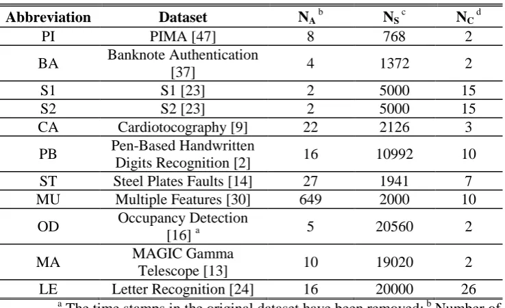
In this subsection, a number of benchmark datasets are used in the performance evaluation as tabulated in Table 1. During the experiments, we assume that we do not have any prior knowledge about the benchmark datasets. The following well-known algorithms are used for comparison:
i) MS: Mean-shift clustering algorithm [19]; ii) SUB: Subtractive clustering algorithm [18]; iii) DBS: DBScan clustering algorithm [21]; iv) SOM: Self-organizing map algorithm [34];
v) ELM: Evolving local means clustering algorithm [20]; vi) DP: Density peaks clustering algorithm [43];
Table 1. Details of the Benchmark Datasets for Evaluation
Abbreviation Dataset NA
b
NS c
NC d
PI PIMA [47] 8 768 2
BA Banknote Authentication
[37] 4 1372 2
S1 S1 [23] 2 5000 15
S2 S2 [23] 2 5000 15
CA Cardiotocography [9] 22 2126 3
PB Pen-Based Handwritten
Digits Recognition [2] 16 10992 10
ST Steel Plates Faults [14] 27 1941 7
MU Multiple Features [30] 649 2000 10
OD Occupancy Detection
[16] a 5 20560 2
MA MAGIC Gamma
Telescope [13] 10 19020 2
LE Letter Recognition [24] 16 20000 26
a
The time stamps in the original dataset have been removed; b Number of attributes; c Number of samples; d Number of classes.
The free parameters and prior assumptions required by the algorithms are listed in Table 2. The free parameter settings used in the experiments by the algorithms are also presented in this table. Due to the very limited prior knowledge during the experiments, the values of these free parameters as listed in Table 2 are determined by the recommendations and/or the experimental settings in the published literature to maximize performance of the datasets. In contrast, our approach does not utilize any of this knowledge, as it is self-organizing and autonomous.
In order to objectively compare the performance of different algorithms, we consider the following measures:
i) Number of data clouds/clusters (C), which should be equal or larger than the number of classes in the dataset;
ii) Calinski Harabasz index (CH) [15], which is used to estimate the optimal number of clusters; the higher the Calinski Harabasz index is, the better the clustering result is;
iii) Mean Silhouette coefficient (SI) [44], which is an indication of how well each sample lies within its cluster. The value range of this index is from -1 to 1. Mean Silhouette coefficient should also be as high as possible.
iv) Time: The execution time (in seconds), which directly indicates the computational complexity and should be as small as possible.
Table 2. Comparison of User Inputs and/or Prior Assumptions between Different Algorithms
Algorithm Free Parameter(s) Prior
Assumption Parameter Setting
ADP none none no need
MS i) bandwidth, p ii) kernel function type
Gaussian distribution
i)p= 0.15 [20] ii) Gaussian kernel SUB initial cluster radius, r Gaussian
distribution r= 0.3 [18]
DBS
i) cluster radius, r ii) minimum number of data samples within the radius, p
Gaussian distribution
i) the value of the knee point of the sorted p-dist
graph ii)p=4 [21]
[image:13.595.84.512.609.769.2]ELM initial cluster radius, r Gaussian
distribution r=0.15 [20] DP i) minimum distance, ρ
ii) local density value, δ
Gaussian distribution
i) relatively high, ρ ii) high, δ [43] NMM i)prior scaling parameter
ii) kappa coefficient
Gaussian
distribution predefined[11] a
NMI grid size Gaussian
distribution predefined [36] CEDS
i) microCluster radius, r ii) decay factor, ω iii) min microCluster threshold, φ
none
i)r= 0.15 ii) ω=500 iii)φ=1 [29] a
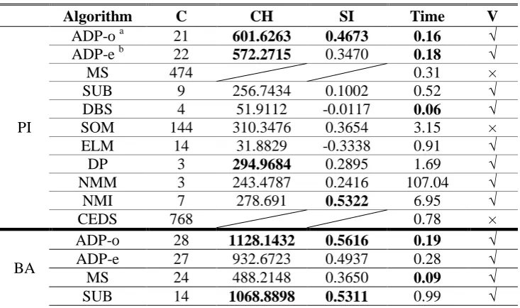
The parameters are fixed in advance The quality measures of performance of the algorithms in terms of C, CH, SI and time based on the benchmark datasets listed in Table 1 are tabulated in Table 3, where we further bold the top three of each performance measure in the experiments for visual clarity.
Ideally, the number of data clouds/clusters generated should be equal or close to the number of classes (ground truth) in the dataset. However, in real situations, especially in the cases of large-scale and/or high dimensional datasets, data samples from different classes are more often mixed with each other, and data samples from the same class may spread into different locations far away from each other in the data space. The best way to deal with such datasets is to partition/cluster the data samples into smaller data clouds/clusters, and combine them later. Therefore, in this paper, we only require the numbers of data clouds/clusters in the clustering results to be close to the ground truth but larger than the number of classes, but not excessively large [28]. Therefore, we consider the clustering result with C meeting the following condition as a valid one:
C S
N C N a (22) In this paper, we consider a3 as a generic value that is not user- or problem-dependent. The rationale is that it indicates an extreme case when each cluster, on average, has only3 members. In this case, the clustering/partitioning result provides too many trivial clusters and is not understandable for users. If CNC, it implies that the clustering algorithm fails to separate the data samples from different classes.
[image:14.595.115.482.544.761.2]Therefore, we additionally add an extra column titled “V” to Table 3 indicating the Validity of the clustering results, where “√” denotes that the clustering result is valid, “×” denotes the invalid one.
Table 3. Numerical Experiment Results on the Numerical Datasets
Algorithm C CH SI Time V
PI
ADP-o a 21 601.6263 0.4673 0.16 √
ADP-e b 22 572.2715 0.3470 0.18 √
MS 474 0.31 ×
SUB 9 256.7434 0.1002 0.52 √
DBS 4 51.9112 -0.0117 0.06 √
SOM 144 310.3476 0.3654 3.15 ×
ELM 14 31.8829 -0.3338 0.91 √
DP 3 294.9684 0.2895 1.69 √
NMM 3 243.4787 0.2416 107.04 √
NMI 7 278.691 0.5322 6.95 √
CEDS 768 0.78 ×
BA
ADP-o 28 1128.1432 0.5616 0.19 √
ADP-e 27 932.6723 0.4937 0.28 √
MS 24 488.2148 0.3650 0.09 √
DBS 48 352.5907 0.2138 0.18 √
SOM 144 1125.6221 0.5828 4.31 ×
ELM 1 54.69 ×
DP 2 723.7514 0.3877 2.57 √
NMM 4 787.2835 0.3718 170.46 √
NMI 20 690.5714 0.4894 6.74 √
CEDS 120 163.6131 0.1709 5.67 ×
S1
ADP-o 15 22675.2540 0.8803 1.09 √
ADP-e 84 6178.3721 0.5949 0.99 √
MS 13 0.03 ×
SUB 10 2.62 ×
DBS 32 14877.9431 0.5851 2.24 √
SOM 144 14891.8742 0.5412 11.88 √
ELM 1 0.78 ×
DP 2 4.08 ×
NMM 6 814.18 ×
NMI 6 15.44 ×
CEDS 21 1285.7427 0.2913 11.85 ×
S2
ADP-o 18 12109.9581 0.7609 1.05 √
ADP-e 65 4813.5951 0.5554 0.97 √
MS 13 0.05 ×
SUB 10 2.39 ×
DBS 35 3406.5872 0.2992 2.22 √
SOM 144 9575.3768 0.5215 11.47 √
ELM 1 0.77 ×
DP 2 5.11 ×
NMM 9 958.76 ×
NMI 4 16.81 ×
CEDS 26 1324.1078 0.2399 12.96 √
CA
ADP-o 71 393.01630 0.3699 0.47 √
ADP-e 45 447.0620 0.3088 0.46 √
MS 3 41.7123 0.3353 0.18 √
SUB 73 235.8645 0.1459 5.77 √
DBS 11 24.3466 0.0377 0.52 √
SOM 144 330.5136 0.3361 7.12 ×
ELM 2 0.48 ×
DP 2 2.41 ×
NMM 3 445.4341 0.4161 257.86 √
NMI 175 272.1408 0.1288 40.35 ×
CEDS 77 272.1408 0.1288 6.55 √
PB
ADP-o 79 1057.9771 0.3821 6.22 √
ADP-e 92 967.5478 0.3206 2.22 √
MS 8493 156.55 ×
SUB 187 382.6055 0.0113 82.98 √
DBS 38 385.3319 -0.0780 12.95 √
SOM 144 864.3771 0.2954 48.27 √
ELM 9 16.78 ×
DP 3 12.53 ×
NMM 41 980.6707 0.3190 7883.89 √
NMI 4316 2331.22 ×
CEDS 1 2466.47 ×
ADP-e 34 11745.7686 0.6613 0.35 √
MS 1 0.78 ×
SUB 1 0.85 ×
DBS 14 3910.0867 0.7920 0.34 √
SOM 144 30043.6256 0.4979 7.84 ×
ELM 1553 1.43 ×
DP 2 2.48 ×
NMM 2 77.99 ×
NMI 6 12.35 ×
CEDS 18 24574.0909 0.7859 7.06 ×
MF
ADP-o 63 618.6775 0.3474 2.96 √
ADP-e 78 414.2603 0.2513 1.19 √
MS 4 2.59 ×
SUB 1994 282.27 ×
DBS 5 1.51 ×
SOM 144 422.4845 0.2598 233.13 ×
ELM 1 0.48 ×
DP 2 4.28 ×
NMM 1 722.11 ×
NMI 1 1892.13 ×
CEDS 90 229.8913 -0.0274 47.97 √
OD
ADP-o 18 34653.4935 0.7608 18.11 √
ADP-e 131 21530.3617 0.3573 4.03 √
MS 20 4291.6125 0.5733 0.10 √
SUB 9 19878.6811 0.3408 16.35 √
DBS 208 1995.0598 -0.6614 36.73 √
SOM 144 81402.2929 0.5776 51.05 √
ELM 1 1.17 ×
DP 2 5495.9202 0.6418 48.45 √
NMM 4 8017.4665 0.5216 2617.14 √
NMI 15 10922.5114 0.7368 396.67 √
CEDS 13 1555.1093 0.0898 42.22 √
MA
ADP-o 47 1430.4657 0.4120 17.68 √
ADP-e 380 643.6832 0.2081 3.86 √
MS 1472 16.2135 -0.4401 48.58 ×
SUB 8 1730.7881 -0.1783 31.54 √
DBS 15 17.8876 -0.4656 37.15 √
SOM 144 1257.2603 0.2344 72.12 √
ELM 25 334.6816 -0.0155 28.55 √
DP 1 44.68 ×
NMM 4 2381.0536 0.5746 2486.65 √
NMI 1578 19.4133 -0.1805 6050.48 ×
CEDS 54 406.1227 -0.2991 5976.02 √
LE
ADP-o 235 433.4874 0.3045 21.99 √
ADP-e 242 414.5848 0.2793 4.28 √
MS 7620 224.92 ×
SUB 153 471.2221 0.2026 154.50 √
DBS 51 94.7283 -0.3547 42.10 √
SOM 144 622.6495 0.2897 99.38 √
ELM 9 17.55 ×
DP 2 53.55 ×
NMI 14526 5768.78 ×
CEDS 43 569.9774 0.0376 13109.01 √
a
The ADP algorithm-offline version; b The ADP algorithm-evolving version.
In the experiments, for the high dimensional datasets (N>20, N=NA), we normalize the data via the following equation, which converts the Euclidean distance between data samples into a cosine dissimilarity [28]:
normalized
x x x (23) We apply the following feature re-scaling operation on the low dimensional datasets (N<20) for the MS , ELM and CEDS algorithms [20],[29]:
min
max min
i i
i
normalized i i
x x x
x x
(24)
where i denotes the ith dimension of the data,
1,2,...,
i N; xmaxi and
min
i
x are the maximum and minimum values of the ith attribute of the data. Note that, the Calinski Harabasz indexes of the results obtained by these two algorithms are calculated based on de-normalized results.
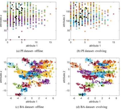
(a) PI dataset- offline (b) PI dataset- evolving
[image:17.595.76.499.308.687.2](c) BA dataset- offline (d) BA dataset- evolving
Fig. 5. The data partitioning results (“o” in different colours denote data samples of different data clouds, “*” denote local modes)
5.2 Experiments on Image Datasets
As it was stated in section 1, clustering techniques are widely used in image analysis. In this subsection, we also conduct several experiments on image clustering. The details of the benchmark image sets used in this subsection are tabulated in Table 4.
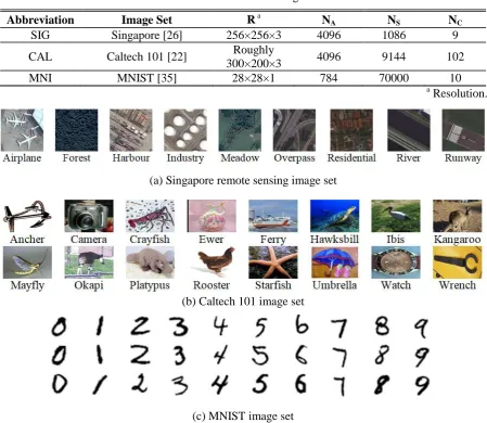
[image:18.595.73.523.208.598.2]Singapore image set [26] is a recently introduced benchmark dataset for remote sensing scene classification. Caltech 101 image set [22] is widely used as a benchmark for object recognition. MNIST image set [35] is the most widely used large scale dataset for handwritten digits recognition. Examples of these images are given in Fig. 6.
Table 4. Details of the Benchmark Image Sets for Evaluation
Abbreviation Image Set R a NA NS NC
SIG Singapore [26] 256×256×3 4096 1086 9
CAL Caltech 101 [22] Roughly
300×200×3 4096 9144 102
MNI MNIST [35] 28×28×1 784 70000 10
a
Resolution.
(a) Singapore remote sensing image set
(b) Caltech 101 image set
(c) MNIST image set
Fig. 6. Illustrative examples of the images used in the experiments
Due to the wide variety of semantic contents and complex textural information contained in the images, separating images of different classes is very difficult. It is of great importance for a clustering/partitioning algorithm to be able to demonstrate strong separation ability. Therefore, for the image clustering problems, we involve an additional clustering quality measure, Purity (PU), which is calculated based on the result and the ground truth indicating the separation ability [20]:
1 PU
C i D i
S K
(25)where i D
[image:19.595.81.514.229.536.2]S is the number of data samples with the dominant class label in the ith cluster. The higher purity the clustering result has, the stronger separation ability the clustering algorithm exhibits.
Table 5. Image Clustering based on Feature Vectors
Algorithm C CH SI PU Time V
SIG
ADP-o 161 15.9752 0.1698 0.9871 3.54 √
ADP-e 97 21.4609 0.1460 0.9678 18.20 √
MS 1085 19.33 ×
SUB 1086 198.26 ×
DBS 2 0.95 ×
SOM 144 17.1072 0.1529 0.9853 473.30 √
ELM 804 126.70 ×
DP 2 3.93 ×
NMM No result generated after 10 hours ×
NMI 1086 17242.22 ×
CEDS 1086 400.17 ×
CAL
ADP-o 1083 12.3015 0.0785 0.8372 289.22 √
ADP-e 441 24.6957 0.0567 0.8074 2362.12 √
MS 9094 2511.28 ×
SUB 9139 7770.47 ×
DBS 40 71.00 ×
SOM 144 64.8208 0.1435 0.7730 4630.92 √
ELM 1110 3.3999 -0.1791 0.4389 4205.27 √
DP 24 123.07 ×
NMM No result generated after 10 hours ×
NMI No result generated after 10 hours ×
CEDS No result generated after 10 hours ×
For the MNIST image set, due to the much simpler structure and semantic contents of the handwritten digit images, we can conduct the image clustering by using the pixels directly. In the following experiment, we convert each image from a 28×28 pixel matrix into a 1×784 pixel vector, and use the pixel vectors as the input to the clustering algorithms. The clustering results on the MNIST image set are tabulated in Table 6. However, as both the cardinality and dimensionality of this image set are very high, the computation- and memory-efficiency of the offline and incremental algorithms deteriorate dramatically due to the iterative learning process. Therefore, in this experiment, we only involve the clustering/data partitioning algorithms, which are non-iterative and “one pass”, namely, the evolving version of ADP, ELM and CEDS.
Table 6. Image Clustering based on Pixel Values
Algorithm C CH SI PU Time V
MNI
ADP-e 4569 31.7081 0.0636 0.9547 9603.45 √
ELM 3 18.11 ×
6. Analysis and Discussion
In this section, we will analyse the performance of the proposed algorithm, and compare it with 8 other well-known algorithms based on the numerical examples presented in section IV.
i) MS algorithm [19]
MS algorithm is very fast when the scale and dimensionality of the dataset is low. However, its calculation speed decreases quickly in processing large scale and high dimensional datasets. The quality of its clustering results varies dramatically. Without prior knowledge, it produced invalid clustering results on many datasets. This is due to its gradient nature making it highly dependent on initial guess and being prone to fall into local minima [19].
ii) SUB algorithm[18]
The calculation efficiency of the SUB algorithm [18] is also largely dependent on the scale and dimensionality of the dataset. It is very inefficient with large-scale and high-dimensional datasets. The clustering results also vary a lot. This algorithm is able to perform high quality clustering on low-dimensional and large-scale datasets. In other cases, however, it failed to give valid and/or useful clustering results.
iii) DBS algorithm[21]
DBS algorithm [21] is an efficient incremental online algorithm. The results it produced generally contain smaller number of clusters. However, the quality of its clustering results is very low. One may also notice that, DBScan algorithm is not effective in handling high-dimensional and large-scale datasets.
iv)SOM algorithm [34]
SOM algorithm [34] requires the size of its net to be pre-fixed and, thus, always produces results with the same number of clusters. The pre-fixed net size enabled the algorithm to perform high quality clustering on high- dimensional and large-scale datasets. However, its calculation efficiency is much lower and it failed to give useful clustering results on small-size datasets.
v) ELM algorithm [20]
ELM algorithm [20] was exhibiting high quality clustering performance on small-scale datasets. However, it did not give any useful clustering results on low-dimensional and large-scale datasets. In complex problems, the algorithm failed to separate the data samples of different classes.
vi) DP algorithm [43]
DP algorithm [43] does not require any prior knowledge in advance, however, during the operation, users need to make choices based on a decision graph generated from the data, namely, to choose one of the rectangles corresponding to the proper minimum distance between centres and local density value. Different choices can lead to very different results and there could be thousands of rectangles generated from datasets with huge size and high dimensionality, which makes it impossible for users to select.
Moreover, using the recommended selection, the algorithm failed to separate the data samples of different classes for high-dimensional and large-scale datasets.
vii) NMM algorithm[11]
NMM algorithm [11] is one of the so-called “nonparametric” algorithms in the comparison despite having a number of pre-defined parameters and coefficients.
viii) NMI algorithm[36]
NMI algorithm [36] is also a so-called “nonparametric” approach. Similarly to the mixture model clustering algorithm [11], it has a number of pre-defined parameters, i.e. grid size, interval between two grids, and it assumes that the data has a Gaussian distribution. This algorithm is very accurate when the datasets are small and the structure is simple.
However, it provided invalid results in processing large-scale and high dimensional datasets. Moreover, its computation efficiency is also largely influenced by the size and dimensionality of the data.
ix)CEDS algorithm [29]
CEDS [29] is a recently introduced algorithm for streaming data clustering. This algorithm can follow the changing data pattern of the data stream and group the samples into arbitrary shaped clusters. Nonetheless, based on the recommended experimental settings, this algorithm is only effective on lower dimensional and/or smaller size datasets, and it frequently fails on complex problems. Its computation efficiency is also very low on large-scale problems.
x) ADP algorithm
As a real algorithm that is free from user- and problem- specific parameters, the proposed ADP algorithm is able to consistently provide high quality clustering results without any user inputs or prior assumptions. Both versions (offline and evolving) are highly efficient computationally and they are very effective in handling datasets with different scale and dimensionality. The indexes measured from the clustering results are all highly ranked compared with the other 9 comparative algorithms used for comparison. From the rank in Tables 3, 5 and 6 one can see that the proposed algorithm is always ranked in the top 3. The computation time is also within the fastest. It is critically important to notice that the proposed algorithm is autonomous, user- and problem- parameter free. In addition, it can evolve its structure to follow the changing data pattern, while others are not. In addition, from the numerical examples one can notice that, the proposed algorithm exhibits even higher effectiveness and efficiency in handling large-scale and higher dimensional datasets compared with other algorithms.
The strong performance of the proposed ADP algorithm comes from a fundamentally different data processing approach based on rank operators. Rank operators are normally avoided in clustering because they are non-linear operators, and so most clustering algorithms prefer the linear mean operator. We believe that the specificity of the rank operator plays a central role in the creation of more parsimonious partitions, specifically when augmented with local mode definitions that are parameter free. Although computationally more demanding, on line rank updates are still practical as we show in our work. For the offline version, the ADP algorithm identifies prototypes from the data samples based on their ranks in terms of the data densities and mutual distances instead of the commonly used means and variances, and use the prototypes to aggregate data samples around them forming Voronoi tessellations [41]. For the evolving version of the ADP algorithm, it has a more flexible evolving structure compared with other online approaches due to its prototype-based nature. In addition, it replaces the pre-defined threshold, which is commonly used in other online approaches, with a dynamically changing threshold derived from the data. Therefore, the ADP algorithm is able to obtain a more stable, effective and objective partitioning compared with other approaches.
7. Conclusion and Future Work
In this paper, a novel algorithm for data partitioning, named autonomous data partition (ADP), was introduced. Both, the offline and evolving versions of the ADP algorithm are entirely data-driven, autonomous and require no user- and problem- specific input. Using nonparametric operators, the proposed algorithm is able to identify the local modes representing the local maxima of the density based on the empirically observed data samples. It partitions the data space into the shape- and parameter-free data clouds. Compared with the well-known algorithms, the proposed approach has the following significant advantages:
i) It is free from prior assumptions and user- and problem- specific parameters;
ii) It is able to conduct high-quality clustering in a short time without the need of prior knowledge. Numerical experiments conducted with the benchmark datasets demonstrate the validity of the proposed algorithm and also show its advantages compared with the alternative well-known algorithms. Moreover, the advantages of the ADP algorithm are even more pronounced on larger size, higher dimensional, complex problems.
As future work, we will study the local optimality and convergence of the ADP algorithm. We will also apply the proposed algorithm to more complex problems, i.e. remote sensing scene image analysis, high frequency trading, etc., and study the underlying data patterns behind them.
Appendix
Web Link
Codes
ADP Algorithm http://empiricaldataanalytics.org/downloads.html Pre-trained
VGG-VD-16 convolutional neural network [46]
http://www.vlfeat.org/matconvnet/pretrained/
Datasets
PIMA [47] https://archive.ics.uci.edu/ml/datasets/pima+indians+diabetes Banknote
Authentication [37] https://archive.ics.uci.edu/ml/datasets/banknote+authentication S1 [23] http://cs.joensuu.fi/sipu/datasets/
S2 [23] http://cs.joensuu.fi/sipu/datasets/
Cardiotocography [9] https://archive.ics.uci.edu/ml/datasets/cardiotocography Pen-Based Handwritten
Digits Recognition [2]
https://archive.ics.uci.edu/ml/datasets/Pen-Based+Recognition+of+Handwritten+Digits Steel Plates Faults [14] http://archive.ics.uci.edu/ml/datasets/steel+plates+faults
Multiple Features [30] https://archive.ics.uci.edu/ml/datasets/Multiple+Features Occupancy Detection
[16] https://archive.ics.uci.edu/ml/datasets/Occupancy+Detection+ MAGIC Gamma
Telescope [13] https://archive.ics.uci.edu/ml/datasets/magic+gamma+telescope Letter Recognition [24] https://archive.ics.uci.edu/ml/datasets/letter+recognition
Singapore [26] http://icn.bjtu.edu.cn/Visint/resources/Scenesig.aspx Caltech 101 [22] http://www.vision.caltech.edu/Image_Datasets/Caltech101/
Acknowledgment
This work was partially supported by The Royal Society grant IE141329/2014 “Novel Machine Learning Paradigms to address Big Data Streams”.
Reference
[1] S. Aeberhard, D. Coomans, and O. de Vel, “Comparison of classifiers in high dimensional settings,” Dept. Math. Statist., James Cook Univ., North Queensland, Australia, Tech. Rep 92-02, 1992.
[2] F. Alimoglu and E. Alpaydin, “Methods of combining multiple classifiers based on different representations for pen-based handwritten digit recognition,” in Proceedings of the Fifth Turkish Artificial Intelligence and Artificial Neural Networks Symposium, 1996, pp. 1–8.
[3] P. Angelov and R. Yager, “A new type of simplified fuzzy rule-based system,” Int. J. Gen. Syst., vol. 41, no. 2, pp. 163–185, 2011.
[4] P. Angelov, Autonomous learning systems: from data streams to knowledge in real time. John Wiley & Sons, Ltd., 2012.
[5] P. Angelov, “Outside the box: an alternative data analytics framework,” J. Autom. Mob. Robot. Intell. Syst., vol. 8, no. 2, pp. 53–59, 2014.
[6] P. P. Angelov, X. Gu, J. Principe, and D. Kangin, “Empirical data analysis - a new tool for data analytics,” in Proceedings of IEEE International Conference on Systems, Man, and Cybernetics, 2016, pp. 53–59.
[7] P. Angelov and P. Sadeghi-Tehran, “Look-a-Like: A Fast Content-Based Image Retrieval Approach Using a Hierarchically Nested Dynamically Evolving Image Clouds and Recursive Local Data Density,” Int. J. Intell. Syst., vol. 32, no. 1, pp. 82–103, 2016. [8] P. Angelov, X. Gu, and D. Kangin, “Empirical data analytics,” Int. J. Intell. Syst., vol. 32,
no. 12, pp. 1261–1284, 2017.
[9] D. Ayres-de-Campos, J. Bernardes, A. Garrido, J. Marques-de-Sa, and L. Pereira-Leite, “SisPorto 2.0: A program for automated analysis of cardiotocograms,” J. Matern. Fetal. Med., vol. 9, no. 5, pp. 311–318, 2000.
[10] J. C. Bezdek, R. Ehrlich, and W. Full, “FCM: The fuzzy c-means clustering algorithm,” Comput. Geosci., vol. 10, no. 2–3, pp. 191–203, 1984.
[11] [D. M. Blei and M. I. Jordan, “Variational inference for Dirichlet process mixtures,” Bayesian Anal., vol. 1, no. 1 A, pp. 121–144, 2006.
[12] D. Birant and A. Kut, “ST-DBSCAN: An algorithm for clustering spatial-temporal data,” Data Knowl. Eng., vol. 60, no. 1, pp. 208–221, 2007.
[13] R. K. Bock, A. Chilingarian, M. Gaug, F. Hakl, T. Hengstebeck, M. Jiřina, J. Klaschka, E. Kotrč, P. Savický, S. Towers, A. Vaiciulis, and W. Wittek, “Methods for multidimensional event classification: A case study using images from a Cherenkov gamma-ray telescope,” Nucl. Instruments Methods Phys. Res. Sect. A Accel. Spectrometers, Detect. Assoc. Equip., vol. 516, no. 2–3, pp. 511–528, 2004.
[14] M. Buscema, “Metanet*: The theory of independent judges.,” Subst. Use Misuse, vol. 33, no. 2, pp. 439–461, 1998.
[15] T. Caliński and J. Harabasz, “A dendrite method for cluster analysis,” Commun. Stat. Methods, vol. 3, no. 1, pp. 1–27, 1974.
[16] L. M. Candanedo and V. Feldheim, “Accurate occupancy detection of an office room from light, temperature, humidity and CO2 measurements using statistical learning models,” Energy Build., vol. 112, pp. 28–39, 2016.
[17] Y. Cheng, “Mean Shift, Mode Seeking, and Clustering,” IEEE Trans. Pattern Anal. Mach. Intell., vol. 17, no. 8, pp. 790–799, 1995.