A Graph Model Proposal for Convex Non Linear
Separable Problems with Linear Constraints
Jaime Cerda, Alberto Avalos
Abstract—The solution of non linear problems are based on very well grounded mathematical theories. This document proposes a Newton step graph-based model for convex non linear separable problems (NLP) with linear constraints. The Newton step is well suited for this kind of problems, but when the problem size grows the NLSP model will grow in a non linear manner. Furthermore, the constraints handling becomes the main problem as we have to select the right constraints in the different solution steps. When this happens, the sparse matrix representation is the path to follow, but very little has been made in order to fully explode the sparsity structure. Indeed, the Hessian matrix for the NLSP model has a very particular structure which can be exploited by using the graph underlying the problem, this is the approach taken in this document. To this end a graph is built derived from the components involved in the Newton step. which describes the solution for the NLSP problem. Based on this graph, the gradient can be evaluated directly based on the graph topology, as it will be shown, the information needed for such evaluation is embedded within the graph. Furthermore, the explicit graph model derived from the mathematical model allows us to think about it in terms of its structure which will be used in further works.
Index Terms—Non Linear Programming, Linear Constraints, Graph-based Systems, KKT Conditions.
NOMENCLATURE
N Number of decision variables.
L Number of equality constraints.
M Number of inequality constraints.
zi Decision variable i.
!zi" Upper limit value of variablezi.
#zi$ Lower limit value of variablezi.
zi Slack variable forzi uppper bound.
zi Slack variable forzi lower bound.
∆zi Variablexi increment.
f(z) Objective function
gl(z) Equality constraintl.
hm(z) Inequality constraintm.
ali ith coefficient in equality constraint l.
bmi ith coefficient in inequality constraintm.
rl RHS of equality constraint l.
sm RHS of inequality constraintm.
λl Dual variable for equality constraint l.
µm Dual variable for inequality constraintm.
ρi Dual variable forzi uppper bound.
ρi Dual variable forzi lower bound.
℘(S) Power set of set S.
Γi Set of variables connected to zi.
Manuscript received July 23, 2013; revised August 6, 2013. This work was supported by the Scientific Research Coordination, Universidad Michoacana de San Nicolas de Hidalgo
J. Cerda ([email protected]) and J. Avalos ([email protected]) are with the Electrical Engineering School, Universidad Michoacana de San Nicolas de Hidalgo, Morelia, Michoacan, Mexico
I. INTRODUCTION
Non linear separable problems (NLSP) are NLPs whose objective function can be decomposed as a sum of functions with only one variable each. The solution of NLSPs are based on very well grounded mathematical theories [1]. This document proposes a Newton step graph-based model for convex non linear separable problems (NLP) with linear constraints. The Newton step is well suited for this kind of problems, but when the problem size grows the NLSP model will grow in a non linear manner. Furthermore, the constraints handling task becomes the main problem as we have to select the right constraints in the different solution steps. When this happens, the sparse matrix representation is the path to follow, but very little has been made in order to fully exploit the sparsity structure. Indeed, the Hessian matrix for the NLSP model has a very particular structure which can be exploited by using the graph underlying the problem, this is the approach taken in this document. To this end a graph is built derived from the components involved in the Newton step. which describes the solution for the NLSP problem. Based on this graph, the gradient can be evaluated directly based on the graph topology, as it will be shown, the information needed for such evaluation is embedded within the graph. Furthermore, the explicit graph model derived from the mathematical model allows us to think about it in terms of its structure which will be used to derive more efficient models as well as decentralization tasks. Finally, even that this model is for convex models it has to be remarked that when used with non convex models this will find local minimizers.
II. A GRAPH-BASED MODEL FOR CONVEXNLSP
In this section a graph topology for the Newton step method is proposed. For this purpose, let us base the discus-sion with the NLSP described by Eq. 1 . This NLSP consists
of N variables, L equality constraints, and M inequality
constraints.
minz
i
!N i=1fi(zi)
st. gl(z) = 0, l= 1,2, ..., L (1)
hm(z) ≤ 0, m= 1,2, ..., M
where fi(zi) are non linear functions, furthermore, we
as-sume they have second order derivatives. On the other hand,
gl(z) are linear equations while hm(z) linear inequalities
L
"
l=1
alizi = rl
M
"
m=1
bmizi ≤ sm
In general, a NLP solver starts by building the Lagrangian given by Eq. 2.
L(z) = N
"
i=1
fi(zi) + L
"
l=1
λlgl(z) + M
"
m=1
µmhm(x) (2)
This is the base to implement the Newton step, whose formulation is given by Eq. 3 [1]:
H(L(z))∆z=−∇(L(z)) (3)
Table I, shows the involved elements to compute the Newton step for problem 1. Do notice we have introduced slack variables as well dual variables which are used to
control the bounds of the decision variables. ρi andzi are
used for the lower bound while ρi andzi are used for the
upper bound of zi
This model can be represented with the graph shown in figure 1.
!"#
$ %'"& $!"& %'"#
(
& ) &
#
# #
#
# # #
#
# #
&
&
& &
#
# #
!'
(
)
-- "1 " " "
1
" " "
) )
)
) )
) )1
# #
#
#
*
# #
#
# # # #
# #
-!& &
* *
-#
& !&
#
* #
)1
)
#
# n
) ) )
" "
"
1
"
#
- # !
# #!
- # !
)
)
# # *
*
!
! &
1
)
# )
# 1
"&
&
Fig. 1. Proposed topology for the Newton step method
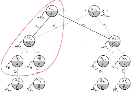
Each constraint is represented by a dual variable and a set of links which represent the linear terms within the con-straint. The terms in the constraints are represented by links which join the primal variables with the dual variables. The only difference between equality contraints and inequality constraints is the kind of links used to build the linking structure. In the case of equality constraints, the linking structure will be active along the whole solution process. On the other hand, the linking structure for the inequality contraints will be active only when the constraint is binding. This is represented by the gray color given to the links belonging to inequality constraints as opposed to the black links which belong to equality constraints. In table I, the
same criterion has been imposed in the elements ofH(L(z)).
As it can be noticed, it is full of empty spaces and gray color, the first are long term sparsity patterns and the second ones are temporary sparsity patterns awaiting to be exploited.
! " !&$% "#$%
&$' #$'
-!
! ! !
(1
( ( (
( ( (
" "
"1
"1 " " "
- -
-)
(
)
& #
%
% %
'
'
' '
% %
%
% %
% %
% %
% '
(
'
' '
"
1
!(
!
(1
' #
#
*
*
% !
(
(
! !
-!!
!
# !
-!
"1 " " "
( (
(
n !
!(
1
(
!
* ! !' '
!
-- - * *
' !'
--
-! !
! !
! !
! ! !
*
Fig. 2. Subgraph for a primal variable (i.e.zl).
III. SELFCONTAINEDGRAPHS
An interesting fact when this kind of graphs is used is that the information to build and compute the gradient is contained in the graph topology. First, the case where the
gradient for a primal variable,zi, is analysed. The discussion
will be focused on the subgraph delineated in figure 2. From
table I, it is known that∇zi =∇fi(zi)−λl−µm−ρi+ρi.
Figure 3 shows the gradient evaluation process for a primal variable. Let us suppose that every node has the value related to the variable which itself represents. Therefore, the node gradient evaluaton starts by taking into account the gradient information within the node which in this case would be
∇fi(zi), as shown in figure 3(a).
Then it starts to evaluate the portion of the gradient which is a function of the variables contained by the neighbours of
zi, as shown in figures from 3(b) to 3(e).
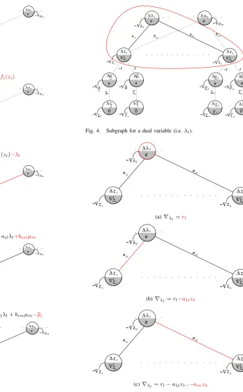
Now, let us turn the attention to the case where the gradient
for a dual variable is to be found, λl in this case. The
discussion will be focused on the subgraph delineated in figure 4.
Figure 3 shows the gradient evaluation process for a dual
variable. From table I it is known that∇λl=rl−z1l−..−
znl. As before, the gradient evaluation starts by taking into
account the information contained within the node itself, in
this caserl, as shown in figure 5(a). Then the evaluation of
the links attached to this node and the variables at the other extreme of the link is performed as shown in figures 5(b) and 5(c)
From the previous discussion, as there exist only dual variables and primal variables, the gradient for every variable can be derived straightforwardly from the graph topology. Therefore, the graph can be said to be self-contained as no external information is needed.
IV. KARUSH-KHUN-TUCKERCONDITIONS
The Langrange multipliers method define optimality con-ditions for equality constraints. However, many problems are defined in terms of inequality constraints defined by 4.
min
z f(z)
st. gl(z) = 0, l= 1,2, ..., L (4)
[image:2.595.312.540.54.217.2] [image:2.595.53.284.393.552.2]L(z) =PNi=1fi(zi)−PLl=1λlgl(z)−PMm=1µmhm(z)
∇(L(z)) H(L(z))
zi λl µm ρi ρi zi zi zi ∇zifi(zi)−λl−µm−ρi+ρi ∇(L(z))z2i ali bmi −1 1
λl gl(z) ail
µm hm(z) bim
ρ
i #zi$ −zi+zi
2/2
−1 zi
ρi zi− %zi&+zi2/2 1 zi
zi ρizi zi ρi
zi ρizi zi ρi
TABLE I
THENEWTON STEP INGREDIENTS
To face this problem, Karush-Khun-Tucker conditions (KKT) generalize the Langrange multipliers method defining a minimum set of conditions which guarantee the optimality conditions for non lineal programming problems with in-equality constraints. Furthermore, KKT conditions provide sufficient optimality conditions for convex programming
problems, as the one we are dealing with. Ifz∗is the optimal
solution for a non lineal problem withN decision variables,
L equality constraints and M inequality constraints, these
conditions are [1]
∇f(z∗) +
L
"
l=1
λl∇gl(z∗) + M
"
m=1
µm∇hm(x∗) = 0 (5)
gl(z∗) = 0, l= 1,2, .., L (6)
hm(z∗) ≤ 0, m= 1,2, .., M (7)
µmhm(z∗) = 0, m= 1,2, .., M (8)
µm ≥ 0, m= 1,2, .., M (9) Where Eq. 5 represents equilibrium between the gradients of the objective function and the active constraints. Equa-tions 6 and 7 represent the feasibility of the solution in the
optimum pointz∗. Equation 8 represent the complementarity
conditions (i.e. µm = 0 or hm(z∗) = 0). Finally, Eq. 9
represents dual feasibility.
Condition 9, establishes the Lagrange multipliers non negativity property. If the Lagrange multiplier was a negative,
thenz∗is within the feasible region, not at the boundary, and
is even feasible to improve the objective function. Therefore, we can conclude that its corresponding constraint is not active anymore. This condition is exploited to discriminate the active from the non active parts of the graph.
V. GRAPHANALYSIS
A node and the links which are attached to it represent an equation. In this section the analysis for a node and the equation it represents is done. To this end let us extract
the equation corresponding to zi from the system of linear
equations which describes the Newton step. This is given by Eq. 10.
∂2
L(z)
∂2z i
∆zi+
"
∀j∈Γi
∂2
L(z)
∂zi∂zj
∆zj =−∇ziL(z) (10)
solving for∆zi leads to
∆zi =
−∇ziL(z)−
!
∀j∈Γi
∂2L(z) ∂zi∂zj∆zj
∂2L(z)
∂2zi
(11)
This can be rewritten as
∆zi= −∇ziL
(z)
∂2L(z)
∂2zi
− "
∀j∈Γi
∂2L(z) ∂zi∂zj
∂2L(z)
∂2zi
∆zj (12)
This expression can be thought as the improvement in the
solution for the component in the orthogonal axiszi. It can be
split into two parts. The first part, described by expression 13, is a component which involves the gradient and, therefore, it is needed within any solution approach for the graph.
−∇ziL(z)
∂2L(z)
∂2zi
(13)
This is the contribution based on−∇ziL(z)just like in the
steepest descent methods. However the length of the step will be reinforced with the second order information provided
by1/∂2∂L2z(iz). This will be the case for the primal variables,
however for the dual variables there will not be second order information, and therefore the gradient step size will have to be controlled by some other means.
The second part, described by expression 14, is composed by all the second order contributions which will be collected
byzi from its neighbours (i.e.Γi).
− "
∀j∈Γi
∂2L(z) ∂zi∂zj
∂2L(z) ∂2zi
∆zj (14)
This part has several of components which will allow us to formulate models which can go from taking into account the second order information from all the neighbors to the other extreme where no second order information from them will be collected at all. The first approach would be the full centralised Newton step and the second one would result in the steepest descent reinforced with the second order information for the same orthogonal axis. Nevertheless, between these two approaches there is a plethora of options which involves a different number of the components of
second order information. In fact there are |℘(Γi)| choices
and the choice at any point will impact the precision of the Newton step and therefore the convergence. Let us define
Lk as the set of links which are taken into account for this
process, do notice |Lk| = k. In fact k = 0 denotes the
steepest descent reinforced with second order information
for the same orthogonal axis whereas k=|Γi| denotes the
!"# $ % &"# ' ( !( !1 "# # #! 1 " ! ) ! -! -# !# ! ) !( 1 " 1 " -!# ! !! -!! ) ) & & # 1
(a)∇zi=∇fi(zi)
!"#
$&"# %
1 !# # --! -! ' ! " ( & # # # " 1 !) ! )1 # ! ! ' ' ! ! -!! ! # !
-"1 "
1 ) !
' !
(b)∇pg=∇fi(zi)−λl
!"#
$&"# %
1 !# # --! -! ' ! " ( & # # # " 1 !) ! )1 # ! ! ' ' ! ! -!! ! # !
-"1 "
1 ) !
' !
(c)∇pg =∇fi(zi)−ailλl+bimµm
!"#
$&"# %
1 !# # --! -! ' ! " ( & # # # " 1 !) ! )1 # ! ! ' ' ! ! -!! ! # !
-"1 "
1 ) !
' !
(d)∇pg =∇fi(zi)−ailλl+bimµm−ρi
!"#
$&"# %
1 !# # --! -! ' ! " ( & # # # " 1 !) ! )1 # ! ! ' ' - !! !! ! # !
-"1 " 1 ) !
'
!
(e)∇pg =∇fi(zi)−ailλl+bimµm−ρi+ρi
Fig. 3. Graph-based gradient evaluation for a primal variable (i.e.zi).
∆zi= −∇ziL
(z)
∂2L(z) ∂2zi
− "
∀j∈Γi (i,j)∈Lh
∂2L(z) ∂zi∂zj
∂2L(z) ∂2zi
∆zj (15)
VI. CONCLUSIONS
This document has presented a graph model proposal for convex non linear separable problems with linear constraints. It has been set the ingredients involved in the Newton step,
! "&$% !#$% "&$' #$'
( % ) % ' ' ' ' ' ' ' ' ' ' % % % % ' ' ' !& ( )
-- "1 " " "
1
" " "
) )
)
) )
) )1
# # # # * # # # # # # # # # -!% % * * -# % !% # * # )1 ) # # n ) ) ) " " " 1 " # - # ! # #! - # ! ) ) # ' * * # # % 1 ) # ) # 1 "% %
Fig. 4. Subgraph for a dual variable (i.e.λl).
a a l,n l,1 -!z 1 z ! -2 z 2 l " n 1 !z ! z1 1 0 n ! z ! " ! -n !
(a)∇λl=rl
a a l,n l,1 -!z 1 z ! -2 z 2 l " n 1 !z ! z1 1 0 n ! z ! " ! -n !
(b)∇λl=rl−a1lz1
a a l,n l,1 -!z 1 z ! -2 z 2 l " n 1 !z ! z1 1 0 n ! z ! " ! -n !
(c)∇λl=rl−a1lz1..−ainzn
Fig. 5. Graph-based gradient evaluation for a dual variable (i.e.λl).
[image:4.595.181.530.45.608.2] [image:4.595.311.541.202.603.2] [image:4.595.89.291.680.731.2]to compute the gradient directly from the graph, provided the correct information is attached to each node. Finally, it has been presented an analysis of the equation represented by the node and its links. This analysis uncovered different patterns to compute the Newton step with different precision levels ranging from the gradient oriented model reinforced with its proper second order information to the full Newton step model where all the second order information terms are taking into account. Furthermore, in between there is a plethora of models which can be derived which will allow more efficient models as well as decentralized models to face problems such as those in [2], [3], [4].
REFERENCES
[1] I. Griva, S. G. Nash, and A. Soferr,Linear and nonlinear optimization. SIAM Society for Industrial and Applied Mathematics, 2009. [2] G. Cohen, “Optimization by decomposition and coordination: A unified
approach,”IEEE Transactions on Automatic Control, vol. 2, no. 2, pp. 222–232, 1978.
[3] A. Bakirtzis, P. N. Biskas, N. Macheras, and N. Pasialis, “A decen-tralized implementation of dc optimal power flow on a network of computers,”IEEE Transactions on Power Systems, vol. 20, no. 1, pp. 25–33, February 2000.