Data pre processing/model initialisation in neurofuzzy modelling of structure property relationships in Al Zn Mg Cu alloys

Published in: ISIJ INTERNATIONAL, VOL 39, (10), 1999, pp. 1027-1037.

DATA PRE-PROCESSING / MODEL INITIALISATION IN

NEUROFUZZY MODELLING OF STRUCTURE-PROPERTY

RELATIONSHIPS IN AL-ZN-MG-CU ALLOYS

O.P. Femminella

, M.J. Starink

, M. Brown

, I. Sinclair

, C.J. Harris

and P.A.S. Reed

1_{Dept. of Engineering Materials, University of Southampton, Southampton S017 1BJ, UK} 2_{Dept. of Electronics and Computer Science, University of Southampton, Southampton S0171BJ, UK}

ABSTRACT

The paper deals with the application of multiple linear regression and neurofuzzy modelling approaches to 7xxx series based aluminium alloys. 36 compositional and ageing time variants and subsequent proof strength and electrical conductivity measurements have been studied. The input datasets have been transformed in two ways: to reveal more explicit microstructural information and to reflect some empirical findings in the literature. Neurofuzzy modelling exhibited improved performance in modelling proof strength and electrical conductivity c.f. the multiple linear regression approach. Electrical conductivity is best modelled using the explicit microstructural input dataset, whilst proof strength is best modelled by a further modification of this dataset, decided upon after inspection of the subnetwork structures produced by neurofuzzy modelling. Neurofuzzy modelling offers a transparent empirically based data-driven approach that can be combined with pre-processing of the data and initialising of the model structure based upon physical understanding. An iterative modelling approach is defined whereby data-driven empirical modelling approaches are first used to assess underlying data structures and are validated against physically based understanding, these then inform subsequent initialised neurofuzzy models and input data transformations to provide both optimal subset and feature representation.

Keywords: neural networks, fuzzy logic, microstructure, 7xxx alloys, electrical conductivity.

1. INTRODUCTION

poor2) . One significant drawback however, is the lack of transparency in the modelling process, and this has hindered more widespread use of the techniques. Generally, neural networks are difficult to validate and have little relationship to conventional physical models, although significant research effort has been directed recently towards incorporating existing physical knowledge into these systems and extracting rules. The neurofuzzy (NF) data modelling algorithms used in this work combine mathematically rigorous non-linear regression-type networks (based on an additive spline representation) with an explanation facility that is based on fuzzy logic, providing a means for combining empirical data with established expert knowledge in both building and validating the model.1) A recent successful NF application concerned Ni-based superalloy fatigue behaviour, which demonstrated that a combination of basic materials’ properties and test conditions readily provided physically reasonable models of near-threshold crack growth.3) Pure neural network models of equivalent data frequently exhibited unrealistic physical characteristics, engendering extensive model interrogation and verification processes.4) _Successful classical neural network modelling of complex materials characteristics has been reported in the literature5,6,7) _{e.g. phase transformation and mechanical property prediction for steels}6,7)_{. This paper} describes a critical progression in the effective use of such methods via the ability to include, ab initio, known physical principles within sophisticated neural network data modelling frameworks, and enables direct assessment of the physical relationships within the transparent models produced.

The dataset considered in the present work contains data on the properties of various Al-Zn-Mg-Cu-Zr based alloys. High strength 7xxx (Al-Zn-Mg-Cu) alloys make up the largest volume of aluminium alloy sold to the aerospace industry and due to the ever increasing demands for property improvement most research and development work of aluminium producers is directed towards this alloy system. 7xxx alloys have 3 critical target properties: yield strength, toughness and stress corrosion cracking (SCC) resistance. SCC is hard to measure on production-line time-scales so generally the more easily obtainable electrical conductivity is used as a measure of SCC resistance. Of the three main properties, yield strength and electrical conductivity are determined mainly by the precipitation processes that occur during commercial thermal treatments of the alloys. The third property, toughness, is a complex function of matrix flow characteristics, intermetallic particle populations (coarse primary constituents and dispersoids), grain structure and coarse heterogeneous precipitation (particularly on boundaries and dispersoids). The balance between the three main properties of 7xxx alloys is a precarious one, with compositional and processing parameters having conflicting effects on the various properties. Modelling of the properties is hampered by the complexity of the relationship between primary process variables (composition, quenching rate, ageing time, ageing temperature, etc.) and target properties, especially toughness and strength. Thus, data for this alloy system is especially suited for investigation using adaptive numerical modelling. Optimal feature representation (data pre-processing) using knowledge of precipitation processes in these alloys may be an effective means of enhancing the predictive capability of models.

2. DATASET

The present, proprietary dataset comprises the results from heat treatment trials carried out by DERA, Farnborough, U.K., under contract from British Aluminium Plate, on a range of alloy compositions that broadly cover the high strength variants of the 7xxx series aluminium alloys. Although of limited size, the dataset reflects its experimentally designed origin as the input distributions were wide ranging if somewhat sparse. For each alloy, composition levels of Zn (xZn,w), Mg (xMg,w), Cu (xCu,w), Zr (xZr,w), Fe (xFe,w) and Si (xSi,w) in wt% have been determined. The alloys were solution treated and subsequently aged for various times at a single temperature which is similar to the ones used for commercial T7 tempers. The subsequent 0.2% proof stress (σ0.2) and electrical conductivity (σel) have been measured for each alloy variant. 36 composition/ageing time variants have been studied, and as a result this dataset can be considered relatively small for the successful application of ANN type approaches. For each differing condition a number of experimental tests had been carried out, mean property measurements have been used throughout.

The inputs (and outputs) were transformed to have a zero mean and unit variance. This simple form of pre-processing is beneficial as it removes non-essential sources of collinearity, improving the condition of the dataset and allowing comparison of magnitudes of the weights determined in the multiple linear regression (MLR). To preserve commercial confidentiality, all data involving input variables has been presented in this normalised form, final output (property) values and mean squared error (MSE) values are however presented in un-normalised form. In the NF modelling framework, in order to facilitate model refinements, which require exact specification of locations (knot placements) along the fuzzified input variables, the input variables are transformed to lie within ±1.

3. EMPIRICAL DATA MODELLING

3.1 Neurofuzzy Data Modelling

rij: IF(x1 is A1i AND x2 is A2i AND … AND xn is Ani) THEN (y is Bj) cij (1)

Where x_k is the kth _{real-valued input, y is the output (model prediction), r}

ij is the ijth fuzzy rule, Aik

is the univariate linguistic term (or fuzzy set) and Bj is the corresponding output linguistic rule.

E.g.: IF (Cu is high) AND (ageing time is medium) THEN (proof stress is high)

Associated with each rule is a rule confidence, cij, which is a measure of the degree of the contribution of the rule to the output. A rule confidence of zero means that the rule does not contribute to the output, and a rule confidence of one means that the rule is completely true. The set of fuzzy sets used to represent an input, and the functions used to express these sets, may be pictorially represented to allow easy interpretation. A simple example of this, with three triangular (second order) fuzzy sets and a variable (e.g. ageing time) with value range 0-10 is shown in Fig 1. At any given value of the variable, membership of all the possible sets adds to unity. For example, at a value of 2.5 the membership of the set “short” is 0.5, of the set “medium” is 0.5 and of the set “long” is zero. The point at which the membership of two fuzzy sets comes to zero (at a value of 0.5 in this case) is called a “knot”, and is likely to represent a change in the trend between input and output. The actual shape of the trend between input and output is determined by the rule confidence.

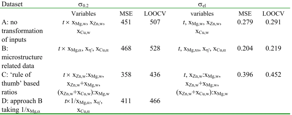
Neurofuzzy modelling combines such qualitative, rule-based representation of the derived model with the structural and learning abilities commonly associated with ANNs. The modelling abilities can be assessed, the structure analysed and standard algorithms can be used to train weights and investigate various structural configurations within a model hypothesis testing framework.9) _The NF modelling employs an analysis of variance (ANOVA) representation to model the additive structural relationships that may exist in the data. This allows the network’s output (predicted properties) to be expressed as a sum of a number of small NF systems (or subnetworks), each with a limited number of inputs (e.g. compositional variables, ageing time) from the main input vector. The output is given by:

( )

( )

( )

( )

( )

s i i p i i i p i i A p i q j c j ij

A c y w a w s

y x

∑

∑

∑

∑

∑

= = = = = = = = = 1 1 1 1 1 μ

where μ_Ai

( )

th _{multivariate fuzzy membership function generated by fuzzy intersection of}

the linguistic variables Aik, yjc is the centre of the jth fuzzy output set and wi is the weight

associated with the corresponding membership function. This representation is identical to a B-spline network, where the multivariate basis functions, ai(x), are the multivariate fuzzy

membership functions. Output si(xi) is the output from the ith subnetwork whose input vector xi is a

smaller subset of the total input vector X. The structure of this type of network is shown in Fig 2.

Each subnetwork is implemented as a conventional NF model, where the output is formed from a linear combination of fuzzy input basis functions which are implemented as B-spline piecewise polynomial basis functions. This simplified additive network reduces the resources (quantity of data) required to implement a robust fuzzy system (compared to one large network taking all the input variables), and gives improved generalisation ability, while also increasing the transparency of the network by simplifying the linguistic fuzzy rules produced.10) _{In addition, when the} subnetworks each have a small number of inputs (1 or 2), the additive structure can reveal simple trends in the network’s output by enabling visualisation of the output of each subnetwork. This is especially important for verification and validation as this can be compared to simple linear models and can highlight regions of differing trends that can be verified against expert knowledge. The NF framework allows the designer to use their own expertise to formulate rules to initialise the network and also to verify relationships extracted from the data by the network against their current physical understanding of the system. This is in contrast to the physically ambiguous character of pure neural networks, which can be seen as “black-box” learning systems.

3.2 Model construction and training neurofuzzy networks

• Univariate addition: inclusion of an input by including another additive subnetwork;

• Tensor product: inclusion of an input to an existing subnetwork, allowing input variable

interactions;

• Knot insertion: the flexibility of a subnetwork is increased by refining the rulebase through

introduction of a new basis function;

• Subnetwork deletion: an existing subnetwork is removed;

• Tensor splitting: a subnetwork with n ≥ 2 inputs is replaced by one that depends on less

combinations of the n inputs;

• Knot deletion: the flexibility of a subnetwork is reduced by reducing the number of basis

functions;

• Reduce order: the order of basis functions in a subnetwork is reduced.

These refinements are combined, to provide a coherent model search, into a forward selection-backward elimination (FS/BE) pass structure, in which initially the overall model structure is identified by a set of model building passes and subsequent model pruning passes are employed to remove any redundant sources of variance, to give the most parsimonious model. Parsimonious models are desirable as each redundant input variable in a network increases its complexity without adding any useful information to the model. Typically an ANN will use mean squared error (MSE) as a measure of prediction performance, where MSE= 1

N (ti −yi) 2

i N

∑

data modelling statistical significance measures are used to balance the network’s MSE against its size and the amount of available data. This ensures that an acceptable level of performance is achieved with respect to the network’s size and the quantity of the available training data.9) The network construction algorithms are stopped when the statistical significance measure starts to rise. To overcome problems associated with finding local minima in MSE and statistical significance, model search termination criteria were appropriately set.11)

In light of empirical results11) the

structural risk minimisation (SRM)12) _{principle was adopted as the statistical significance measure.} Due to the small sample size, the order of the B-splines considered was limited to be ≤ 2, to prevent the inclusion of severely ill-conditioned basis functions.

For a given set of inputs and corresponding output(s) the network can be trained in either of the following ways:

• the training data are presented to an initially empty model and the automatic model construction algorithms search for the network structure;

• the data can be presented to an initial network structure which reflects prior knowledge and

system understanding and network construction algorithms used to refine the model structure;

• connections and rule bases (model structure) can be defined and the network left to determine only the weights/rule confidences.

paper. The network was then presented with these two revised datasets to examine to what degree the incorporation of “expert knowledge” at the data pre-processing stage would improve the modelling performance. All data available was used in the model construction to retain the maximum possible information. Models constructed were assessed in terms of their statistical significance measure (SS), an adjusted training set MSE taking into account the number of parameters (nw) fitted in the model. Once the model was identified, a leave-one-out cross-validation (LOOCV) strategy was employed to assess the generalisation performance of the model, by estimating the model’s prediction error. Since model identification was determined using all the

data available, the LOOCV estimate of prediction error will still exhibit some bias. Target output (measured properties) versus model output (predictions) were also examined. Relationships identified were validated against known physical metallurgy principles.

From examination of the models identified by the automatic model construction algorithms and using a priori knowledge of the likely physical processes and trends characterising alloy behaviour, model initialisation was investigated, by specifying a prior functional form for the model (i.e. specifying a set of fuzzy rules). The three datasets (A, B and C) were then presented to this predetermined model structure so that the efficacy of the data pre-processing could be assessed further.

3.3 Multiple linear regression analysis

To provide a benchmark against which the NF modelling approaches can be assessed, a multiple linear regression was also carried out on each dataset. A linear model is given by equation (3):

( )

y = + + +_L+

2 2 1 1

0 (3)

where x = [x1,..., xp]T is the model’s input vector, w1,...,wp are unknown fitting parameters to be estimated, w0 is an unknown bias term and y is the predicted output. The unknown vector of parameters, wp, can be estimated in the least squares sense.

The next section of the paper details and justifies the two data pre-processing approaches adopted to further improve the modelling process.

4. TRANSFORMATION OF INPUT VARIABLES

4.1 Precipitation in Al-Zn-Mg-Cu Alloys

A large body of work on the thermodynamics, microstructure and microstructure-property relations of 7xxx (Al-Zn-Cu-Mg) type alloys exists.13,14,15,16,17,18,19,20) _{Using this knowledge, modelling of the}

strength of ternary Al-Zn-Mg alloys on an analytical microstructure related basis21) _{has been}

main phases. In the interest of clarity, we have limited ourselves to considering just two microstructural elements: the volume fraction of the main strengthening phase η' that forms in the alloys and the volume fraction of the main coarse intermetallic phase: the S (Al2MgCu) phase.

4.2 Main microstructure related strengthening and conductivity effects

During homogenising and solution treatments some of the Cu and Mg present in the 7xxx alloys will not dissolve in the Al-rich matrix because some S (Al2MgCu) phase will be stable at the solution treatment temperature. The Cu and Mg “tied-up” in the S phase will thus not cause any increase in σel of the Al-rich phase (the Al-rich phase is the only significant conductive pathway in the alloys) and, further, are not available for subsequent precipitation hardening during ageing (precipitation hardening is the dominating strengthening mechanism). This means that, in first approximation, the Cu and Mg present in S phase have become largely irrelevant in affecting the σel and σ0.2 of the alloy. (However, the S phase will have a detrimental effect on a third important mechanical property: the toughness.) Thus, modelling of σel and σ0.2 of the alloy variants may be improved by transforming the atomic fraction of Cu and Mg, xCu and xMg into xCu,α and xMg,α, the

atomic fraction of Cu and Mg dissolvable in the Al-rich (α) phase. The latter quantities can be obtained as follows.

If the stochiometry of a phase is fixed, the solubility of an intermetallic phase can often be described by the regular solution model.13,22,23) _{In this model the solvus related to an intermetallic} phase MmAaBbCc (M is the main constituent of the alloy, and A, B, C are the alloying elements) is given by:

( ) ( ) ( )

A exp (4)

where ΔHsol is the enthalpy of formation of one ‘molecule’ of MmAaBb, kB is Boltzmann’s constant and co is a constant. If appropriate values for ΔHsol, co, a, b and c for each phase can be derived from available solubility data, a phase diagram can be constructed. However, only for T=460ºC significant data on the solvi of all phases are available.16) For the S phase the Hsol(S) in ternary alloys has been determined previously23), and by combining solvus data at 460ºC16) with Hsol the S solvus as a function of the temperature can be estimated. For S phase, at the solution treatment temperature applied to the present alloys, it is thus estimated:

( )

( )

Cu Mg c

c (5)

xCu,α and xMg,α can then be calculated as follows:

if

( )

( )

Cu Mg x

x then xCu,α= xCu and xCu,α= xCu (6)

if

( )

( )

Cu Mg x

then 2 4 2

1 2

1

, =− ( Mg − Cu)+ ( Mg − Cu) −4×2.9610

Cu x x x x

x _α

and x_Mg,α =x_Mg −

(

)

and the atomic fraction of S phase is given by:

xS =4(xCu −xCu,α) (8)

Whilst several precipitation sequences in 7xxx alloys have been reported, it is well established that the main sequence responsible for most of the age-hardening in 7xxx alloys is:

sssα → GP zones → η' → η (9)

η' is thought to have a stochiometry close to Mg4Zn11Al24) whilst η is based on MgZn2.14,24) For peak aged and overaged alloys, η' will be the main hardening phase and, hence, the maximum atomic fraction of η' that can form is given by:

⎟⎟ ⎠ ⎞ ⎜⎜ ⎝ ⎛ = 4 , 11 min 16 , η' α Mg Zn x x

x (10)

It is thought that for the modelling of σ0.2, xη' is the main composition related variable. Additionally, xCu,α and xMg,α are expected to have an influence, mainly through solution

strengthening of the alloy. Of the latter two xMg,α is thought to have the stronger influence on the

strength, as solution strengthening due to Mg is generally considered to be more important than that due to Cu.25,26)

It is further known that the amount of Mg that is left in solution after completed formation of the main precipitate(s) is an important parameter determining the properties of overaged alloys27)_{. We} have calculated this so-called “excess Mg”, xMg,xs, using a novel expression, which is, at present, proprietary. Also xη' , xCu,α and xMg,α are expected to have an influence with the Zn content related

xη' parameter having a stronger effect than xCu,α and xMg,α.13)

From the above, it follows that the main variables determining σ0.2 are xη' and t with secondary effects determined by xMg,α and xCu,α. The main variables determining σel are xMg,xs and t with further minor contributions from xCu,α and a very small influence due to xZn (or xη'). Thus in the modelling approaches described below we have applied these insights to construct a new set of input variables relevant to the properties to be modelled (dataset B) consisting of: xη' , t , xMg,α ,

xCu,α , xMg,xs and xs.

4.3 Rule of thumb variables: ratios and sums

xZn,w:xMg,w, (xZn,w+xCu,w):xMg,w and xZn,w+xMg,w. These ratios can have physical meanings, e.g. the xZn,w:xMg,w ratio will exert an important influence on the balance of the main precipitation sequences operating in the alloy, but, in terms of solid state reactions, the relevance of adding weight percentages of atoms is, in general, unclear. However, it can be seen that with the atomic weight of Zn being about 2.7 times that of Mg, adding xZn,w+xMg,w (in weight percentage) may be some measure of the amount of strengthening η' phase, provided this phase has a broad range of stability around its central composition of Mg4Zn11Al. In order to fully investigate possible permutations of input variables we have considered the three sums and ratios xZn,w:xMg,w, (xZn,w+xCu,w):xMg,w and xZn,w+xMg,w, in addition to ageing time, t. These four input variables (and the corresponding output values of σ0.2 and σel) make up dataset C, the “rule-of-thumb” dataset.

5. MODELLING OF THE DATASETS

Both the MLR and the NF modelling approaches have been applied to all 3 datasets (A – raw data, B – microstructure related and C – “rule-of-thumb”).

5.1 Data analysis

Inspection of data distributions, statistical and conditioning diagnostics allowed any collinearity between variables to be identified. Some degree of correlation was found between xFe,w and xZr,w in dataset A and between xZn,w:xMg,w and (xZn,w+xCu,w):xMg,w in dataset C. Two near linear dependencies were detected in dataset B, the first between xCu,α and xS and the second involving xMg,α, xη' and xMg,xs. The collinearities in datasets B and C can be understood directly in terms of the transformations performed in section 4. The correlations in dataset A may be a reflection of the small sample size. Such collinearities are of concern for subsequent regression analyses and inferences, as these data weaknesses will be responsible for high parametric uncertainty and lower confidence in the predictions.

5.2 MLR analysis

Dataset A (raw data)

Dataset B

(microstructure related data)

Dataset C

(“rule-of-thumb” data)

Weights Weights Weights

Inputs

σ0.2 σel

Inputs

σ0.2 σel

Inputs

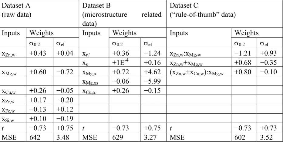
σ0.2 σel xZn,w +0.43 +0.04 xη' +0.36 −1.24 xZn,w:xMg,w −1.21 +0.93

xs +1E-4 +0.16 xZn,w+xMg,w +0.68 −0.35 xMg,w +0.60 −0.72 xMg,α +0.72 +4.62 (xZn,w+xCu,w):xMg,w +0.80 −0.10

xMg,xs −0.06 −5.99 xCu,w +0.26 −0.05 xCu,α +0.26 −0.15

xZr,w +0.17 −0.20

xFe,w −0.13 +0.12

xSi,w +0.10 −0.19

t −0.73 +0.75 t −0.73 +0.75 t −0.73 +0.73

MSE 642 3.48 MSE 629 3.27 MSE 602 3.52

Table 1 Linear regression analysis of the data on σ0.2 and σel employing three different sets of input data: the raw input data (dataset A), the set transformed using microstructure related assessments (dataset B) and the set transformed using “rule-of-thumb” sums and ratios (dataset C)

σ0.2 σel

Dataset Model MSE LOOCV SS nw Model MSE LOOCV SS nw

A Fig.3 451 507 2394 8 Fig.4 0.344 0.385 1.29 5

B Fig.5 544 590 2444 6 Fig.6 0.259 0.271 0.98 5

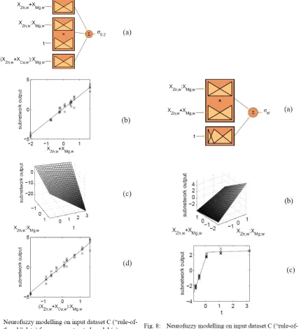
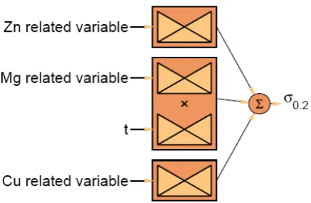
C Fig.7 358 436 1898 8 Fig.8 0.256 0.272 1.41 7

Table 2 Model performance measures for NF modelling of σ0.2 and σel employing three different sets of input data: the raw input data (dataset A), the set transformed using microstructure related assessments (dataset B) and the set transformed using “rule-of-thumb” sums and ratios (dataset C).

5.3 Neurofuzzy data modelling

chosen to model σel: in all 3 cases the ageing time is modelled by a piecewise linear approximation and this extra flexibility has allowed a considerable improvement in the MSE c.f. MLR.

dataset B identifies t and xMg,xs as the main variables influencing σel, which is in accordance with the discussion in section 4.2. The selection of t, xη' and xMg,α as the main variables influencing σ0.2 is again in accordance with section 4.2. One surprising result of the NF model construction for set B is the selection of the tensor product xMg,α × t. In terms of microstructure development this

5.4 Neurofuzzy model initialisation.

Unless an exhaustive search for an optimal model is undertaken, the instability of the heuristic model construction algorithms may mean that the model may still settle in a local minima. In this modelling exercise the small sample size has placed a significant restriction on the number of possible adjustable parameters in the model. Initialising the σ0.2 NF model by including xCu,α in

dataset to the general form in Fig 11 provides a comparison of the effect of the data transformations on modelling σ0.2. Similarly, we may define a general constrained model to compare the effect of data transformations on modelling σel. Comparison of the models in Fig4a, Fig 6a, and Fig 8a shows that the models for σel are generally given by a summation of a piecewise linear approximation to t with (depending on the input dataset) composition related inputs. Hence, a general model incorporating all these features is the one presented in Fig 12.

The relative performance of the three different sets of input data when using the initialised model structures (Fig 11 and Fig 12) is presented in Table 3. In addition to the three sets of input variables (A, B and C) employed thus far we have also included results for a fourth set (set D) which is the same as set B apart from the fact that for the model for σ0.2 instead of xMg,α, 1/xMg,α is

Dataset σ0.2 σel

Variables MSE LOOCV variables MSE LOOCV

A: no

transformation of inputs

t × xMg,w, xZn,w, xCu,w

451 507 t, xMg,w, xZn,w, xCu,w

0.279 0.291

B:

microstructure related data

t × xMg,α, xη', xCu,α 468 528 t, xMg,xs, xη', xCu,α 0.204 0.219

C: ‘rule of thumb’ based ratios

t × xZn,w:xMg,w, xZn,w+xMg,w, (xZn,w+xCu,w):xMg,w

358 436 t, xZn,w:xMg,w, xZn,w+xMg,w, (xZn,w+xCu,w):xMg,w

0.396 0.452

D: approach B taking 1/xMg,α

t×1/xMg,α, xη', xCu,α

411 466

Table 3 Training set MSE and LOOCV prediction MSE estimates obtained for the initialised models for σ0.2 and σel for three different sets of input data: the raw input data (dataset A), the set transformed using microstructure related assessments (dataset B) and the set transformed using “rule-of-thumb” sums and ratios (dataset C) and the 1/xMg,α (dataset D).

6. SUMMARY AND DISCUSSION

6.1 Modelling approaches

A dataset of 7xxx series-based aluminium alloys with 7 input variables (6 alloying element concentrations and ageing time) and 2 output variables (the properties σ0.2 and σel) has been analysed using multiple linear regression (MLR) and NF modelling approaches. For both modelling approaches we evaluated the effectiveness of pre-processing of the input data using 2 types of transformations of the composition variables. In order to facilitate comparisons the root mean square errors (RMSE) on the test data obtained from Tables 1 to 3 are presented graphically in Fig 13. This shows that both for σ0.2 and σel (irrespective of data pre-processing) the NF modelling always yields improved model predictive ability as compared to MLR, with the difference being especially pronounced for σel. These improvements are due to increased flexibility in the models that are constructed in the NF modelling framework which yield a better functional representation than the simple inflexible MLR models. In modelling σ0.2 the NF approach selects a model which contains a sub-model combining t and a Mg-related parameter (xMg,w for set A, xMg,α for set B and xZn,w:xMg,w for set C), and for the modelling of σel the NF approach selects a model which contains a piecewise linear approximation for the t-dependency. As evidenced by the reduced SS and MSE values, these refinements are well matched to the data and the identification of these refinements via a method which is supported by the data is the main advantage in the NF approach when applied to the present dataset.

Dataset B has represented the data in explicit microstructural features so that the specific effects of different microstructure contributions can be assessed. In contrast, for modelling σ0.2, Fig 13 shows that the use of transformed input dataset C is clearly the most beneficial. In this case we still have greater confidence in the trends indicated by the dataset B model, which is more parsimonious (fewest number of adjustable parameters) but shows worse MSE. A modelling cycle has been identified consisting of:

Fig.13: Comparison between training and LOOCV estimates of RMSE for the modelling approaches pursued (MLR, NF, initialised NF models) and data pre-processing (A, B, C).

(1) data inspection/understanding ↔ (2) dataset selection ↔ (3) empirical modelling (model construction) ↔ (4) model validation (physical insight) ↔ (1) etc.

Based on inspection of the FS/BE model constructions, general initialised models were defined for each property with a similar structure (Figures 11 and 12) for each dataset. This formed a basis for comparison of the effects on modelling performance for each dataset transformation. In modelling σ0.2 the initialised model for dataset C showed approximately a 10% reduction in the test RMSE c.f. test RMSEs for datasets A and B; dataset D - produced as a result of the modelling cycle defined earlier and is a combination of physically based transformations (dataset B) and a transformation suggested by inspection of NF model constructions - exhibited an improved test RMSE over dataset B. In modelling σel, the initialised model for dataset B showed at least a 15% reduction in test RMSE c.f. test RMSEs over datasets A and C.

0 10 20 30 40

A B C A B C A B C D

σ0.2 Train

σ0.2 LOOCV

20 x σel Train

20 x _σel LOOCV

6.2 Microstructure-property relations of 7xxx alloys

The present analysis can be used to draw out some of the microstructure property issues for the present, complex 7xxx (Al-Zn-Mg-Cu) alloys. Firstly it is noted that compared to the original untransformed dataset (A) the dataset transformed using some relatively simple information on the microstructure (B) yielded a considerable improvement in NF modelling performance for σel but no improvement in the modelling of σ0.2. In retrospect this difference is not surprising as strength is the more complex property, more dependent on additional microstructural features that are not directly included in the available inputs (e.g. grain size, precipitate size distributions). Both the MLR and the NF modelling confirm the main expected structure-property relationships, for example, the maximum amount of η', xη', is important in determining the strength. In addition the NF approach revealed that for σ0.2, a sub-model of t and Mg concentration improves modelling performance statistics. It is suggested that this sub-model in essence represents the complex interaction of dissolved Mg with vacancies, which will influence the rate of ageing: possibly vacancies bind to the Mg atoms enhancing ageing in the present overaged alloys.

At present the modelling of the properties of 7xxx alloys on the basis of microstructural knowledge is further pursued by combining kinetic equations (e.g. Johnson-Mehl-Avrami-Kolmogorov29,30) _or Starink-Zahra31,32,33) _{type equations), coarsening models and microstructural investigation. Initial} results are promising: further enhancement of the accuracy of model predictions is possible using this approach, where pre-specified regression functions (based on sound physical metallurgy) are being used. This, however, does not detract from the data-driven results reported in the present paper. NF modelling, combined with suitable transformation of input data and model initialisation, is a transparent approach which allows us to gain information about relationships in the data through the modelling process and provides a route by which purely empirical modelling approaches can be combined with physical modelling relatively easily. Such an approach requires only limited knowledge of the system investigated, and is hence an important tool for analysis of complicated materials processing issues.

7. CONCLUSIONS

situations where more limited physical understanding exists, a NF modelling approach offers a combination of pure empirical modelling and physically based modelling possibilities.

8. ACKNOWLEDGEMENTS

Thanks are due to Dr. P.D. Pitcher at MSS, DERA and Dr. J. Newman, British Aluminium Plate for provision of the dataset, financial support from Federal Mogul and the University of Southampton is also gratefully acknowledged.

REFERENCES

1) M. Brown and C.J. Harris: Neurofuzzy Adaptive Modelling and Control, Prentice Hall, (1994).

2) C.J. Harris, M. Brown, K.M. Bossley, D.J. Mills and M. Feng: J. Engng. Apps. AI, 9 (1996), 1. 3) J.M. Schooling, M. Brown and P.A.S. Reed:Mater. Sci. Engng. A, 260 (1999), 222-239.

4) J.M. Schooling and P.A.S. Reed: Proc. of 8th Int. TMS Conf. on Superalloys, Seven Springs, USA, (1996), 409.

5) A. Mukherjee, S. Schmauder and M. Ruhle: Acta Metall. Mater., 43 (1995), 4083-4091.

6) H.K.D.H. Bhadeshia, D.J.C. MacKay and L.-E. Svensson: Mat. Sci. Tech., 11 (1995), 1046-1051.

7) L. Gavard, H.K.D.H. Bhadeshia, D.J.C. MacKay and S. Suzuki: Mat. Sci. Tech., 12 (1996),

453.

8) M. Brown and C. J. Harris: Int. J. of Neural Syst., 6(2) (1995), 197-220.

9) K. M. Bossley: Neurofuzzy modelling approaches in system identification, Ph.D. thesis, Southampton (1997).

10) M. Brown, K.M. Bossley & C. J. Harris: EUFIT ‘96, (1996), vol.2, 762-766.

11) S.R. Gunn, M. Brown & K.M. Bossley: Lecture notes in computer science n.1208, (1997), 313-323.

12) V.N. Vapnik: The Nature of Statistical Learning Theory. Springer-Verlag, New York (1995).

13) R.H. Brown and L.A. Willey, in Aluminium: Properties, Physical Metallurgy and Phase Diagrams, K.R. van Horn, ed. (ASM, Ohio, 1967), 31-54

14) L.F. Mondolfo: Aluminium Alloys, Butterworths & Co Ltd, London (1976).

15) P. Villars, A. Prince and H. Okamoto: ‘ASM Handbook of Ternary Alloy Diagrams’, ASM International, Materials Park, Ohio (1995).

16) D.J. Strawbridge, W. Hume-Rothery and A.T. Little: J. Inst. Metals, 74 (1948), 191-225. 17) H. Liang, S.-L. Chen and Y.A. Chang: Metall. Mater. Trans. A, 28 (1997), 1725.

18) P. Liang, T. Tarfa, J.A. Robinson, S. Wagner, P. Ochin, M.G. Harmelin, H.J. Seifert, H.L. Lukas and F. Aldinger: Thermochim. Acta, 314 (1998), 87.

19) P. Sainfort, C. Sigli, G.M. Raynaud and Ph. Gomiero: Mater. Sci. Forum, 242 (1997), 25-32. 20) T.J. Warner, R.A. Shahani, P. Lassince and G.M. Raynaud: 3rd ASM Conf. on Synthesis,

Processing and Modelling of Advanced Materials, Paris, France, June 1997.

22) M.J. Starink and P.J. Gregson: Scr. Metall. Mater., 33 (1995), 893-900. 23) M.J. Starink and P.J. Gregson: Mater. Sci. Forum, 217-222 (1996), 673-678. 24) J.K. Park and A.J. Ardell: Scr. Metall., 22 (1988), 1115-1119.

25) P. Gomiero, Y. Brechet, F. Louchet, A. Tourabi and B. Wack: Acta Metall. Mater., 40 (1992),

857.

26) M.J. Starink, P. Wang, I. Sinclair and P.J. Gregson: submitted to Acta Mater.

27) K.R. Anderson, US Patent no. 5312498 (1994)

28) M.J. Starink and A.-M. Zahra: Acta Mater., 46 (1998), 3381-3397.

29) J.W. Christian: The Theory of Transformation in Metals and Alloys, 2nd ed., Part 1, Pergamon Press, Oxford, UK, 1975.

30) V. Sessa, M. Fanfoni and M. Tomellini: Phys. Rev. B, 54 (1996) 836.

31) M.J. Starink and A.-M. Zahra: Thermochim. Acta, 292 (1997) 159.

32) M.J. Starink and A.-M. Zahra: Acta Mater., 46 (1998) 3381.