Fast Image Interpolation for Motion Estimation using Graphics Hardware,

Fast Image Interpolation for Motion Estimation using

Graphics Hardware

Francis Kelly and Anil Kokaram

Department of Electronic and Electrical Engineering, University of Dublin,

Trinity College, Dublin 2, Ireland

ABSTRACT

Motion estimation and compensation is the key to high quality video coding. Block matching motion estimation is used in most video codecs, including MPEG-2, MPEG-4, H.263 and H.26L. Motion estimation is also a key component in the digital restoration of archived video and for post-production and special effects in the movie industry. Sub-pixel accurate motion vectors can improve the quality of the vector field and lead to more efficient video coding. However sub-pixel accuracy requires interpolation of the image data. Image interpolation is a key requirement of many image processing algorithms. Often interpolation can be a bottleneck in these applications, especially in motion estimation due to the large number pixels involved. In this paper we propose using commodity computer graphics hardware for fast image interpolation. We use the full search block matching algorithm to illustrate the problems and limitations of using graphics hardware in this way.

Keywords: Image Interpolation, Motion Estimation, Block Matching, Programmable Graphics Hardware

1. INTRODUCTION

Image interpolation is a fundamental requirement for many image and video processing applications. It can however often be a bottleneck in terms of performance for these applications. Motion estimation is one such application where image interpolation can cause a large performance hit. Interpolation is necessary in motion estimation when sub-pel accurate motion vectors are required. Video codecs such as H.263 and MPEG-2 recom-mend using at least 1/2 pel accuracy for the motion vectors. MPEG-4 and H.26L use higher accuracy motion vectors of 1/4 pel and 1/8 pel. For restoration and movie post-production purposes motion vectors with a mini-mum of 1/8 pel accuracy are typically required. Image warping is another application where image interpolation is required.

The type of image interpolation used is normally governed by an accuracy/speed trade-off. As interpolation accuracy increases so does computational cost. In motion estimation algorithms bilinear interpolation is usually a sufficient compromise between interpolation accuracy and speed. This paper concentrates on fast bilinear interpolation for block matching motion estimation. It proposes using the latest in programmable graphics hardware for doing this interpolation quickly.

2. MOTION ESTIMATION

Motion estimation is one of the key components in video processing. It is central to high quality video coding in

standards like MPEG-2, MPEG-4, H.263, H.26L etc. It is also used in the restoration of archive video1 and for

creating special effects in the film industry.2 Accurate real-time motion estimation is currently only possible

on dedicated hardware.3 Motion estimation is also useful for frame rate conversion4 in broadcast television.

High end TV sets have hardware, such as Phillips Melzonic image processing chip,5 which use real-time motion

Further author information: (Send correspondence to F.K.) F.K.: E-mail: [email protected], Telephone: +353 (0)1 608 2202

Address: Department of Electronic and Electrical Engineering, University of Dublin, Trinity College, Dublin 2, Ireland A.K.: E-mail: [email protected], Telephone: +353 (0)1 608 3412

Address: Department of Electronic and Electrical Engineering, University of Dublin, Trinity College, Dublin 2, Ireland Web: http://www.mee.tcd.ie/~sigmedia

estimation and compensation for deinterlacing and scan rate conversion. These chips however can often be impractical or too expensive for use with applications on standard desktop PCs. The goal of this research is to achieve real-time motion estimation using standard desktop PC components at PAL television broadcast rates (720x576 pixels @ 25 frames/sec). In this paper we concentrate mainly on the exhaustive search block matching algorithm.

2.1. Full Search Block Matching

Block matching is the most common approach to motion estimation used today. It is quite simple to implement as it requires highly regular operations which are easily parallelizable. As such it has been implemented in video

coding hardware.3, 5 The image is divided up into blocks of size M ×N pixels, and a motion vector d for

each block in the current frame is estimated by finding the best matching block in a defined search space in the previous frame. The motion model used here is a translational one, and is defined as

I_n(x) =I_n−1(x+d_n,n−1), (1)

where I_n(x) is the grey level of the pixel at the location given by position vectorxin the framen, andd_n,n−1

is a displacement mapping the region in the current framen into the previous framen−1. Using this model,

the intensity of each pixel in the current frame can be predicted from a shifted location of pixels in the previous

frame. The only parameter that is required for this model is the motion vectord.

Block matching algorithms usually search a known set of candidate motion vectors, choosing the motion vector for each block which minimises some function of the Displaced Frame Difference (DFD). The search space

is usually given as±wpixels for the horizontal and vertical components. For integer accurate motion estimation

there are (2w+ 1)2 vectors in the candidate set. For fractional motion vectors there are even more, depending

on the accuracy required. The matching criteria used here is the sum of absolute differences (SAD)

SAD(b,d) = N−1

i=0

M−1

j=0

|DFD(b(i, j),d)|. (2)

The functionbmaps the current block pixel position (i, j) to a pixel in the full image. Rearranging Equation 1

gives us the definition of the DFD at positionxand displacementd

DFD(x,d) =I_n(x)−I_n−1(x+d). (3)

In exhaustive search or full search block matching (FBM) all possible vectors in the search space are checked. This is very computationally intensive. There are many algorithms which attempt to reduce the computational

cost of FBM, such as the Three Step Search6or The Cross Search.7 These algorithms usually reduce the number

of locations searched, by limiting the search space to some pattern, or reduce the number of pixels sampled in

each block.8 While these reduced search techniques can offer large savings in computation, they may find local

minima in the DFD function and yield wrong motion vectors. While this paper only considers the FBM scheme, the techniques described could easily be applied to other block matching algorithms.

2.2. Image Interpolation

Real image sequences typically exhibit non-integer motion. This implies that accurate motion compensation of the scene can not be achieved with a candidate set of integer accurate motion vectors. Sub-pel accurate motion vectors must be included in the set as well. However in order to estimate and compensate fractional pel displacements, the image signal has to be interpolated.

As stated earlier there are (2w+ 1)2 possible motion vectors for integer accurate block matching with a

search space of±wpels. For sub-pel accuracy there are (2w/α+ 1)2 motion vectors in the candidate set, where

0.0 < α≤1.0 is the accuracy required. This is approximately a factor of (1/α)2 increase over the number of

integer vectors to search. Also (2w/α+ 1)2−(2w+ 1)2≈(1/α)2−1 of these vectors have fractional components,

which means that the image must be interpolated to check these vectors. Bilinear interpolation can take up

operations per pixel are required for full search sub-pel accurate motion estimation. For example, an accuracy

of α = 0.5 means approximately 21 extra operations per pixel, and α = 0.25 gives approximately 105 extra

operations per pixel.

In this paper we propose using the latest generation graphics hardware for fast image interpolation to reduce the computational load on the CPU. Consider an image displayed on a PC monitor. Consider further that the image window is then resized. Typically the graphics hardware has to do some form of interpolation of this image to display it correctly at the new resolution. In fact if the image is a texture then the graphics hardware can use bilinear interpolation to provide good quality image resizing. This paper exploits such functionality for general image processing.

3. PROGRAMMABLE GRAPHICS HARDWARE

Modern computer graphics hardware contain extremely powerful graphics processing units (GPU). These GPUs are designed to perform a limited number of operations on very large amounts of data. They typically have more than one processing pipeline working in parallel with each other. They can in fact be thought of as highly parallel Single Instruction Multiple Data (SIMD) type processors.

The performance of these GPUs is also growing at an extraordinary rate. In fact over the last decade or so the processing power of GPUs has been growing at a rate faster than Moore’s Law, which governs the performance

growth rate of CPUs.9 In a presentation at Graphics Hardware 2003 titled “Data Parallel Computing on

Graphics Hardware”, Ian Buck estimated that the current Nvidia GeForce FX 5900 GPU performance peaks at

20 GigaFlops. This is equivalent to a 10-GHz Pentium 4 processor.10

The latest generation of graphics hardware also contain much more programmable GPUs. Previously the number of operations that could be performed on the GPU was limited to certain fixed functions such as Texture and Lighting. However the GPU has evolved to a situation where we now have user programmable vertex and texture units. These are commonly referred to as vertex shaders and fragment shaders respectively. These programmable shaders allow for much more realistic visual effects in computer games especially, which is the main driving force behind the computer graphics hardware industry.

A further improvement in these new GPUs is the increase in pixel depth from 32 bits per pixel to 128 bits per pixel. This means that each red, green, blue, and alpha component can now have 32-bit floating point accuracy throughout the graphics pipeline. This increase in data accuracy combined with the increased programmability of the GPU means that the GPU is moving towards a more general purpose processor design.

In the last few years there has been an increase in research in the area of using graphics hardware for general

purpose computing. Yang and Welch11 show how to perform fast image segmentation and smoothing using

graphics hardware. They implemented functions like erosion and dilation on the GPU. They state that this

implementation is over 30% faster that a similar CPU implementation. Larsen and McAllister12 describe a

technique for doing fast matrix multiplies using graphics hardware. Typically these were very large matrices

There is also an implementation of the Fast Fourier Transform implemented on the GPU.13 They can do the

FFT on a 512x512 resolution image in under a second, fully on the GPU. A good source of information for this

research area can be found athttp://www.gpgpu.org.

3.1. Programming the GPU

The GPU is designed for operating on large continuous streams of vertex and fragment data. Vertices are points in 3-D space which define graphics primitives like triangles, polygons, rectangles etc. These primitives are used to build up the geometry of the scene and define any 2-D or 3-D models to be displayed. In older hardware the geometry sent to the graphics card was static. If this geometry or model data had to be altered in some way, it had to be transformed on the CPU and the new vertices downloaded to the GPU. Vertex shaders were designed to allow more control over vertex transformation on the GPU itself. This has obvious benefits as it frees up the CPU for other processes and also eliminates the need to download the same model over and over again.

mapping stage is after the vertex stage in the graphics pipeline. Fragments are the name given to the data in the pipeline before it gets output as pixels to the screen. Fragments are slightly different than pixels because there can be fragments which will occupy more than one pixel on the screen. At the texture stage the texture image is looked up for the correct color to add to the fragment before it is converted to a pixel(s). Similar to vertex shaders, previous generation hardware texture units were limited in the operations they could perform on fragments. Fragment shaders were introduced to allow much more control of how textures are applied to the fragments. Fragment shaders also tend to be more powerful than vertex shaders as they are usually operating on higher volumes of data. They can also perform memory reads as they look up values in textures.

Pixels are finally rendered at end of the graphics pipeline in a conceptual device called the framebuffer. Generally pixels rendered to the framebuffer are made visible on the screen to the user. However this framebuffer data can become corrupted if other windows on the screen are moved and overlap with the current window. This is because the same framebuffer, which is a piece of GPU memory, is shared for all applications on the desktop. To overcome this problem another useful feature of modern graphics hardware is exploited: off-screen rendering buffers called pixel buffers (Pbuffers). These Pbuffers reside in GPU memory and are similar to the framebuffer, except they are generated and controlled by the application. Also, the framebuffer does not benefit from the increase in pixel depth and is limited to 32 bits per pixel. Pbuffers are necessary if a 128 bits per pixel rendering buffer and floating point computation are required. If further processing of the results generated is needed, the Pbuffer can be used as a texture and passed through the graphics pipeline again.

In order to use the GPU for general purpose computing the problem has to be mapped onto the GPUs programming architecture. In this case per-pixel operations on the GPU are required. The results are then read back to the CPU. To achieve this the images have to be downloaded as textures to the GPU for use in fragment programs. This involves rendering a rectangle and texture mapping the images to this rectangle. If this rectangle is the same size as the images then the fragments will correspond on a one to one basis with the pixels in the texture. Fragment programs can then be used to do the required calculations on the GPU, and results output to a Pbuffer.

For this work the cross platform OpenGL API was used for interfacing with the graphics hardware. The other main graphics API is Microsoft’s Direct X. Programming the GPU involves writing custom vertex and fragment programs to be executed by the vertex and fragment shaders. In this paper the code snippets are written based on the OpenGL ARB vertex and fragment program standard. The language used resembles assembly language for common general purpose processors. The following is the instruction set for fragment programs and it is very similar for vertex programs.

ABS ADD CMP COS DP3 DP4 DPH DST EX2 FLR FRC KIL LG2 LIT LRP MAD MAX MIN MOV MUL POW RCP RSQ SCS SGE SIN SLT SUB SWZ TEX TXB TXP XPD

It is however a limited instruction set with no support for program flow control such as branching or looping. These are features which will probably be implemented in the next generation of graphics hardware. Also fragment programs run independently for each fragment, and are usually operating in parallel on different fragments. This means that there is no way to use the results of one fragment when working on a different

fragment. There are higher level languages such as Nvidia’s Cg14 or Mircosoft’s High Level Shading Language

(HLSL) available. These are similar to the C,C++ type programming languages. They use compilers to generate the appropriate assembly language for the GPU. In this case however the programs are simple enough to be written directly in the assembly language. This also means that the programs can be fully optimised for the underlying hardware and do not use any unnecessary registers or instructions.

3.2. Interpolation on the GPU

0 200 400 600 800 1000 1200 1400 1600 1800 2000 0

0.05 0.1 0.15 0.2 0.25 0.3

Horizontal Resolution (pixels)

Time (secs)

CPU GPU incl readback GPU w/o readback

0 200 400 600 800 1000 1200 1400 1600 1800 2000 0

2 4 6 8 10 12 14

Horizontal Resolution (pixels)

Ratio GPU : CPU

GPU (incl readback) : CPU Mean

GPU (w/o readback) : CPU Mean

(a) (b)

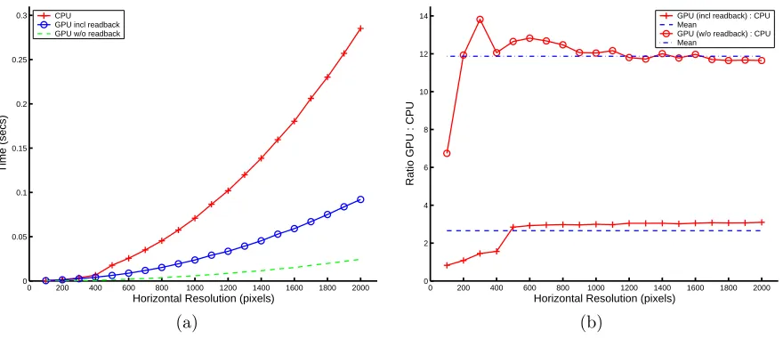
Figure 1.Compensate image by fractional amount using bilinear interpolation. a) Timings for GPU vs CPU. b) Ratio

of GPU to CPU including mean value.

3.2.1. Bandwidth Issues

One of the main bottlenecks when using the GPU for image processing is the time taken to read the data back from the graphics hardware to the CPU. The Accelerated Port Technology (AGP) standard is a means

of transferring data quickly to the graphics hardware. It operates at a multiple of the PCI bus speed; AGP4x

operates at 4 times the PCI bus speed and the latest AGP standard, AGP8x, operates at 8 times the PCI bus

speed. However reading data backfromthe graphics hardware is limited by the standard PCI bus speed. With a

PCI bus speed of 66 MHz the theoretical bandwidth available is approximately 260 MB/sec, whereas the AGP8x bus has a peak bandwidth of 2.1 GB/sec. In tests however a peak data read bandwidth of 180 MB/sec or 45 MPixels/sec at 32bits per pixel was achieved. For PAL resolution frames this gives a peak frame rate of 113 frames/sec for reading data from the graphics card. Downloading the image as a texture, doing the interpolation, and reading the data back resulted in 75 frames/sec at PAL resolution. Doing the same interpolation on the CPU achieved 24 frames/sec. A new PCI bus standard due out in 2004 called PCI Express, may help with this problem by providing greater bandwidth over the PCI bus.

3.2.2. Interpolation Results

Figure 1 (a) compares the time taken to bilinearly interpolate an image using both the GPU and CPU. Two GPU times are shown: one including reading the image data back from the GPU and the other without data readback. Only the horizontal resolution of the images used is shown for clarity, but all images had an aspect ratio of 4:3. Figure 1 (b) gives an indication of the speed up achieved over the CPU when using the GPU for interpolation. Again the two cases for data readback are shown. As can be clearly seen the GPU version is on average almost three times faster than a CPU only version, even with the time taken to read the interpolated image back to the CPU included. The CPU version uses the Intel Performance Primitive libraries which are highly optimised for the extended SSE2 instruction set of the Pentium 4 processor.

Compare this to the time taken to do interpolation on the GPU without reading the data back. In this case the GPU is approximately twelve times faster than the CPU implementation. This shows that almost 75% of the time taken to use the GPU for interpolation is spent on reading the data back from the graphics hardware. This is due to the PCI bottleneck. Based on these results, if data readback bandwidth was the same as the AGP bandwidth, then the GPU would be almost ten times faster for bilinear interpolation than the CPU.

3.2.3. Interpolation Accuracy

−0.40 −0.3 −0.2 −0.1 0 0.1 0.2 0.3 0.4 0.5 0.6 1

2 3 4 5 6 7 8 9 10x 10

4

Pixel Difference between CPU and GPU

Frequency

−0.60 −0.4 −0.2 0 0.2 0.4 0.6 0.8 1 1.2 1

2 3 4 5 6 7x 10

4

Pixel Difference between CPU and GPU

Frequency

(a) (b)

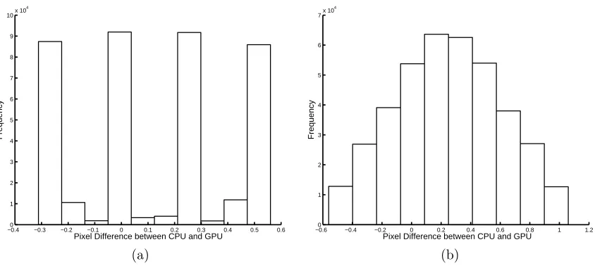
Figure 2. Histogram of errors between bilinearly interpolated images generated on the GPU and CPU. (a) 0.5 pel

accurate interpolation. (b) 0.25 pel accurate interpolation.

the GPU does not produce identical images to those generated on the CPU. These errors appear to be due to slight round-off problems and precision issues on the graphics hardware. In general these slight differences are not a problem. However in certain cases they can lead to the wrong motion vector being chosen for a block, see

section 4.3. Take the case of a 16×16 block of pixels. If there is an error of 0.5 for each pixel in the block, this

can lead to an error of±128 in the SAD for the block.

4. FBM USING THE GPU

The approach taken for FBM on the GPU is slightly different than a CPU implementation. The GPU is designed to work on large volumes of data in parallel. To exploit the GPU hardware efficiently, it is necessary to restructure the standard block matching algorithm. Typically block matching implementations shift blocks around the search space individually, calculating the SAD for each motion vector. On the GPU however it is more efficient to shift the entire frame at once for each motion vector, with the SAD then calculated on a block basis.

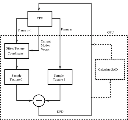
An appropriate algorithm flow for FBM using the GPU as a co-processor for the CPU is shown in figure 3. Firstly the two frames are downloaded as textures to the graphics hardware. These are noted as Texture0 and Texture1 respectively. The current motion vector to be checked is passed as a parameter to the GPU. The DFD for the two frames is then generated using vertex and fragment programs. In this way if a frame needs to be interpolated it will be interpolated on the GPU. This results in an image which is the absolute value of the DFD for the two frames. This image is then read back to the CPU where a SAD measure for each block in the image is generated. This is repeated for each motion vector in our candidate set. The motion vector which yielded the smallest SAD for each block is chosen as the motion vector for that block.

In order to alleviate the PCI bottleneck in data read mode, it is necessary to perform more of the algorithm on the GPU. It is possible to do this by calculating the blocks SAD using fragment programs. This is shown as the dashed option on the data read path in Figure 3. If the SAD is generated on the GPU only one value per

block has to be read back, rather thanN×N pixels for each block. Unfortunately it is only possible to generate

the sum for 2×2 pixels at a time. A recursive algorithm is required where many passes through the pipeline

are necessary to generate the SAD for the N×N block. On each pass 2×2 blocks of pixels are summed and

the image subsampled by a factor of two. Every pass through the pipeline reduces the framerate of the GPU.

Generating the SAD on the GPU in this manner requires log₂N additional passes. However, it is on average

Calculate SAD CPU

DFD

GPU Frame n

Frame n−1

Offset Texture Coordinates

Vector Motion Current

Texture 0 Sample

Texture 1 Sample

Figure 3.Block diagram showing GPU and CPU operation.

4.1. Vertex & Fragment Programs

This first segment of code shows the vertex program used to set up the texture coordinates for the two textures. For clarity only the necessary lines of code are shown. It is these texture coordinates which will be used by the texture units to look up values in the textures. For Texture1 we just pass through the current input position as the texture coordinates (line 12). This is because Texture1 corresponds to the current frame of the video sequence, it does not need to be shifted or interpolated. The current motion vector is passed by the CPU as a parameter to the vertex program (line 6). This is then added to the current input position to generate the offset texture coordinates for Texture0, the previous frame of the video sequence (line 11).

!!ARBvp1.0 ....

2 OUTPUT oTexture0 = result.texcoord[0]; 3 OUTPUT oTexture1 = result.texcoord[1]; 4 ATTRIB iPosition = vertex.position; 6 PARAM vector = program.local[1]; ....

11 ADD oTexture0, iPosition, vector; 12 MOV oTexture1, iPosition;

END

0 0.2 0.4 0.6 0.8 1 0

20 40 60 80 100 120 140 160 180

Accuracy

Time (secs)

CPU GPU (with SAD) GPU (without SAD)

Figure 4.Average time for FBM at different pixel accuracies.

!!ARBfp1.0

1 OUTPUT output = result.color; 2 TEMP frame1,frame2;

3 TEX frame1, fragment.texcoord[0], texture[0], RECT; 4 TEX frame2, fragment.texcoord[1], texture[1], RECT; 5 SUB frame1, frame1, frame2;

6 ABS output, frame1; END

4.2. Results

The results shown here were generated using a 1.6 GHz Pentium 4 machine with a GeForce FX 5600 GPU. In the FBM scheme used all blocks in the image were searched, there was no motion detection used to reduce the number of blocks searched. Also all possible vectors in the search space were checked. This means that the results are a poor indication of the performance of the block matching algorithm. However the goal of this work is to compare the performance of the GPU to that of the CPU for similar heavy computational loads. It is the relative speed increase between a CPU only and a GPU-CPU implementation that is of interest. The search

space was±4 pixels and the block size was 16×16 pixels. The experiments were carried out on the well known

calendar/mobile sequence at PAL resolution.

Figure 4 shows the average time in seconds to do FBM using the GPU and the CPU. As can be seen for integer accurate motion vectors the CPU is faster than the GPU method. Because integer accuracy searching requires no interpolation, a very efficient implementation can be done on the CPU. For sub-pel accurate FBM however, there is a big difference in performance between the two. Generating the DFD on the GPU and reading it back to the CPU is on average 2.5 times faster for FBM than generating the DFD on the CPU. If the SAD for the blocks are calculated on the GPU, FBM is approximately four times faster than the CPU version.

4.3. Accuracy

Two measures are used here to denote the accuracy of the GPU results when compared to a CPU implementation. These are the Peak Signal to Noise Ratio (PSNR) and the Entropy. Using equation 2 and 3, we define the PSNR

for an image of sizeM ×N pixels as

P SNR= 20log₁₀

255

SAD/MN

0 5 10 15 20 25 34.5

35 35.5 36 36.5 37 37.5 38 38.5

Frame Number

PSNR (db)

1.0 pel accuracy 0.5 pel accuracy 0.25 pel accuracy 0.125 pel accuracy

0 5 10 15 20 25

3 3.1 3.2 3.3 3.4 3.5 3.6 3.7 3.8

Frame Number

Entropy

(a) (b)

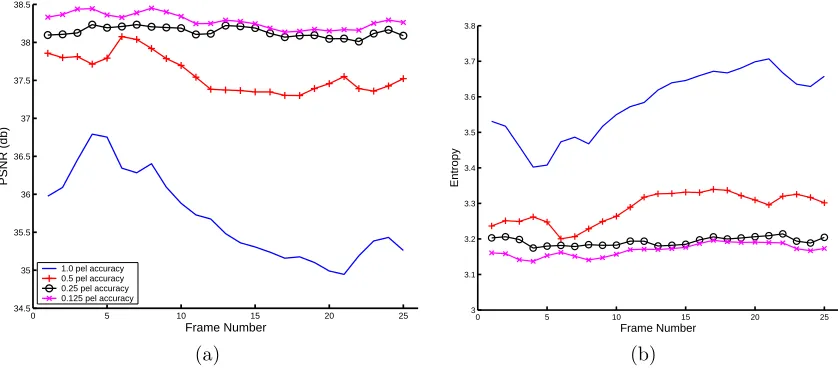
Figure 5.Peak signal to noise ratio and Entropy comparisons for the calendar/mobile sequence at various pixel

accura-cies.

where the SAD is calculated over the whole motion compensated DFD.

Figure 5 (a) shows the PSNR for the calendar/mobile sequence for the various pixel accuracies. For integer accurate motion vectors the results for the CPU and GPU versions are identical. For sub-pel accuracy there is a very slight difference between the CPU and GPU results, which cannot be distinguished on the graph. These plots also show the improvement in PSNR that comes from sub-pel accurate motion estimation. Figure 5 (b) is a graph of the entropy of the motion compensated DFD at different motion vector accuracies. Similar to the PSNR graph, this shows almost identical results for the GPU and CPU implementations. The entropy decreases as motion vector accuracy increases, which should lead to better coding performance.

Figure 6 shows a close up of the PSNR (a), and entropy (b), for the calendar/mobile sequence motion compensated at 0.25 pel accuracy. This shows the slight difference in results between the GPU and CPU implementations of FBM. In this case the mean error between the two is only 0.0042 dB. Figure 7 (b) shows a histogram of the difference between the SAD as calculated on the GPU and the CPU, for a sub-pel accurate

motion vector of d= [1.5,2.5]. As can be seen the majority of SADs are equal, i.e the error is zero. However

due to some errors in the texture interpolation hardware, outlined in section 3.2.3, there will also be blocks for which the SADs are not equal.

This difference in SAD is what causes the different motion vectors shown in Figure 7 (a), and which gives the slight difference in PSNR and entropy between the CPU and GPU. It is mainly in flat areas however that this SAD error causes the motion vectors to be different. This is because in flat image areas there is not enough structural or texturual information to yield a unique match for motion. In such blocks all candidate motion vectors yield similar SAD measures. Therefore a slight change in the SAD for one candidate vector can cause the best motion vector match to change drastically. Some form of motion detection could be used to alleviate this problem by ensuring that a block is in fact moving before finding a motion vector for it. In blocks where there is good image structure a slight difference in SAD has a smaller effect on the motion vector chosen.

5. CONCLUSION

0 5 10 15 20 25 38

38.05 38.1 38.15 38.2 38.25

Frame Number

PSNR (db)

0.25 pel accuracy CPU 0.25 pel accuracy GPU

0 5 10 15 20 25

3.17 3.175 3.18 3.185 3.19 3.195 3.2 3.205 3.21 3.215

Frame Number

Entropy

(a) (b)

Figure 6.Close up of Peak signal to noise ratio and Entropy for 0.25 pel accuracy.

160 176 192 208

16

32

48

64 −400 −30 −20 −10 0 10 20 30 40

20 40 60 80 100 120 140 160 180

SAD error between GPU and CPU

Frequency

(a) (b)

Figure 7. (a) Section of vector field for calendar/mobile sequence. CPU vectors are in black and GPU vectors are in

white. Vectors are scaled for clarity. (b) Histogram of errors between SAD generated by GPU and CPU.

in this paper, the techniques used could easily be applied to other fast search algorithms which require sub-pel accuracy.

We have also outlined one of the main problems while using the GPU for general purpose computing, reading the data back from the graphics hardware. In video processing applications especially, the PCI bus bandwidth is too low for the large amount of data that has to be transferred across it. To overcome this problem we generated the SAD measure on the GPU, to reduce the amount of data read back to the CPU. The introduction of a new PCI bus standard may help alleviate this problem in the future. We also noticed some precision issues in using the GPU for interpolation. The exact cause of this is unknown, although for this application it had little effect on the results.

REFERENCES

2. A. Kokaram, B. Collis, and S. Robinson, “A bayesian framework for recursive object removal in movie

post-production,” inIEEE International Conference on Image Processing, Barcelona, September 2003.

3. Sony CXD19222Q Real Time MPEG-2 Video Encoder, 1997.

4. G. de Haan, P. Biezen, H. Huijgen, and O. A. Ojo, “True-motion estimation with 3-d recursive search block

matching,”IEEE Transactions on Circuits and Systems for Video Technology, pp. 368–379, October 1993.

5. Philips SAA4998WP MELZONIC image processing chip, 1997.

6. T. Koga, K. Iinmua, A. Hirano, Y. Iijima, and T. Ishiguro, “Motion-compensated interframe coding for

video conferencing,” inProceedings NTC’81 (IEEE), pp. G.5.3.1–G.5.3.4, 1981.

7. M. Ghanbari, “The cross-search alogrithm for motion estimation,”IEEE Transactions on Communications.

38, pp. 950–953, July 1990.

8. A. Zaccarin and B. Liu, “Fast algorithms for block motion estimation,” inroceedings of IEEE ICASSP,3,

pp. 449–452, 1992.

9. M. C. Lin and D. Manocha, “Interactive geometric computations using graphics hardware,” in

SIG-GRAPH’02 Tutorial Course 31, 2002.

10. M. Macedonia, “The gpu enters computing’s mainstream,”IEEE Computer, October 2003.

11. R. Yang and G. Welch, “Fast image segmentation and smoothing using commodity graphics hardware,”To

appear in the journal of graphics tools, special issue on Hardware-Accelerated Rendering Techniques, 2003.

12. E. S. Larsen and D. McAllister, “Fast matrix multiplies using graphics hardware,”Supercomputing 2001 ,

November 2001.

13. K. Moreland and E. Angel, “The FFT on a GPU,” inGraphics Hardware 2003, July 2003.

14. W. Mark, R. Glanville, K. Akeley, and M. Kilgard, “Cg: A system for programming graphics hardware in