Copula models in machine learning

(1)

Copula models in

Machine Learning

Inauguraldissertation

zur

Erlangung der W¨

urde eines Doktors der Philosophie

vorgelegt der

Philosophisch-Naturwissenschaftlichen Fakult¨

at

der Universit¨

at Basel

von

M´

elanie Rey

aus Montana, Schweiz

Basel, 2015

Original document stored on the publication server of the University of Basel edoc.unibas.ch

This work is licenced under the agreement

”Attribution Non-Commercial No Derivatives 3.0 Switzerland” (CC BY-NC-ND 3.0 CH). The complete text may be reviewed here:

(2)

Genehmigt von der Philosophisch-Naturwissenschaftlichen Fakult¨at

auf Antrag von

Prof. Dr. Volker Roth, Universit¨at Basel, Dissertationsleiter Prof. Dr. Gal Elidan, the Hebrew University, Korreferent

Basel, den 22.04.2014

(3)

Namensnennung-Keine kommerzielle Nutzung-Keine Bearbeitung 3.0 Schweiz (CC BY-NC-ND 3.0 CH)

Sie dürfen: Teilen — den Inhalt kopieren, verbreiten und zugänglich machen

Unter den folgenden Bedingungen:

Namensnennung — Sie müssen den Namen des Autors/Rechteinhabers in der von ihm festgelegten Weise nennen.

Keine kommerzielle Nutzung — Sie dürfen diesen Inhalt nicht für kommerzielle Zwecke nutzen.

Keine Bearbeitung erlaubt — Sie dürfen diesen Inhalt nicht bearbeiten, abwandeln oder in anderer Weise verändern.

Wobei gilt:

 Verzichtserklärung — Jede der vorgenannten Bedingungen kann aufgehoben werden, sofern Sie die ausdrückliche Einwilligung des Rechteinhabers dazu erhalten.

 Public Domain (gemeinfreie oder nicht-schützbare Inhalte) — Soweit das Werk, der Inhalt oder irgendein Teil davon zur Public Domain der jeweiligen Rechtsordnung gehört, wird dieser Status von der Lizenz in keiner Weise berührt.

 Sonstige Rechte — Die Lizenz hat keinerlei Einfluss auf die folgenden Rechte:

o Die Rechte, die jedermann wegen der Schranken des Urheberrechts oder aufgrund gesetzlicher Erlaubnisse zustehen (in einigen Ländern als grundsätzliche Doktrin des fair use bekannt);

o Die Persönlichkeitsrechte des Urhebers;

o Rechte anderer Personen, entweder am Lizenzgegenstand selber oder bezüglich seiner Verwendung, zum Beispiel für Werbung oder Privatsphärenschutz.

 Hinweis — Bei jeder Nutzung oder Verbreitung müssen Sie anderen alle

Lizenzbedingungen mitteilen, die für diesen Inhalt gelten. Am einfachsten ist es, an entsprechender Stelle einen Link auf diese Seite einzubinden.

(4)

(5)

Abstract

The introduction of copulas, which allow separating the dependence structure of a multivariate distribution from its marginal behaviour, was a major advance in dependence modelling. Copulas brought new theoretical insights to the concept of dependence and enabled the construction of a variety of new multivariate distributions. Despite their popularity in statistics and financial mod-elling, copulas have remained largely unknown in the machine learning community until recently. This thesis investigates the use of copula models, in particular Gaussian copulas, for solving vari-ous machine learning problems and makes contributions in the domains of dependence detection between datasets, compression based on side information, and variable selection.

Our first contribution is the introduction of a copula mixture model to perform dependency-seeking clustering for co-occurring samples from different data sources. The model takes advantage of the great flexibility offered by the copula framework to extend mixtures of Canonical Correlation Analyzers to multivariate data with arbitrary continuous marginal densities. We formulate our model as a non-parametric Bayesian mixture and provide an efficient Markov Chain Monte Carlo inference algorithm for it. Experiments on real and synthetic data demonstrate that the increased flexibility of the copula mixture significantly improves the quality of the clustering and the inter-pretability of the results.

The second contribution is a reformulation of the information bottleneck (IB) problem in terms of a copula, using the equivalence between mutual information and negative copula entropy. Fo-cusing on the Gaussian copula, we extend the analytical IB solution available for the multivariate Gaussian case to meta-Gaussian distributions which retain a Gaussian dependence structure but allow arbitrary marginal densities. The resulting approach extends the range of applicability of IB to non-Gaussian continuous data and is less sensitive to outliers than the original IB formulation. Our third and final contribution is the development of a novel sparse compression technique based on the information bottleneck (IB) principle, which takes into account side information. We achieve this by introducing a sparse variant of IB that compresses the data by preserving the information in only a few selected input dimensions. By assuming a Gaussian copula we can capture arbitrary non-Gaussian marginals, continuous or discrete. We use our model to select a subset of biomarkers relevant to the evolution of malignant melanoma and show that our sparse selection provides reliable predictors.

(6)

List of Figures

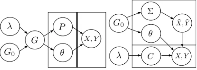
3.1 Graphical illustration of the generative model for meta-Gaussian continuous variables. 37

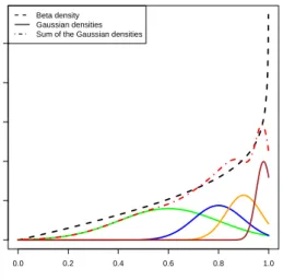
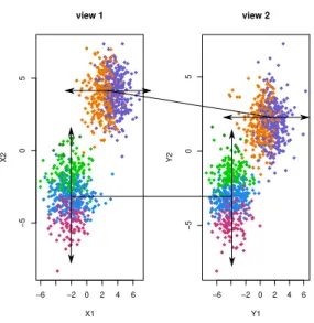
4.1 Gaussian components approximating a beta density. . . 43 4.2 Simulated example of Gaussian data expressing a non-uniform dependence pattern

between views 1 and 2. . . 45 4.3 Graphical representation of the infinite copula mixture model with base measure

G0 and concentrationλ. . . 47

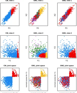
4.4 Scatterplot of the simulated data in the Gaussian view, in the beta view and in the joint space of the normal scores for the two views where the two clusters can be clearly identified. . . 50 4.5 Boxplot of the adjusted rand index over 100 and 50 simulations for the copula

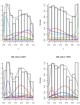
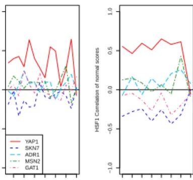
mixture (CM). . . 50 4.6 Histogram of the binding affinity scores for the binding factors GAT1 and YAP1. . 51 4.7 Correlations estimated with GM and correlations of the normal scores estimated

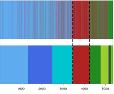
by CM between HSF1 and the five other binding factors. . . 52 4.8 Cluster indices for all genes as obtained using dependency-seeking clustering with

CM and cluster indices obtained when clustering in the complete product space. . 53

5.1 Graphical representation of the conditional independence structure of IB. . . 55

6.1 Information curves for Gaussian data with outliers, data with Student, Exponential and Beta margins. . . 66 6.2 Parzen density estimates of the univariate projection ofXsplit in 5 groups according

to values of the first relevance variable. . . 67

7.1 Objective function f and constraint g. . . 71 7.2 50 (overlapping) information curves for each method and solution paths for the 15

(10)

7.3 Boxplots of the elements Aii in the diagonal projection matrix and Kaplan-Meier

plots of the two patient groups from the test cohort. . . 80 7.4 Solution paths for 9 diagonal entries ofAwhen the roles ofX andY are reversed. 80

(11)

List of Tables

(12)

Acknowledgements

My thesis advisor Prof. Dr. Volker Roth played a crucial role in the development of the work presented here which would not have materialised without his insightful ideas and academic guid-ance. I would like to thank him for his constant support and the many theoretical discussions by which he gave ideas and problems a little more life.

I am very grateful to my co-examiner Prof. Dr. Gal Elidan for reviewing my thesis and feel honored by his interest in my work.

Collaborating with Prof. Dr. Niko Beerenwinkel, Armin Töpfer (ETH Zürich, Basel), Dr. Karin J. Metzner, Dr. Huldrych Günthard, Francesca Di Giallonardo (University Hospital, Zürich) and Dr. Osvaldo Zagordi (University of Zürich, Zürich) was a privilege and an enriching experience. I would like to thank my colleagues Sandhya Prabhakaran, David Adametz, Behrouz Tajoddin, Dinu Kaufmann, Julia Vogt and Sudhir Raman for their support and friendship. A special thought goes to Sandhya for the countless moments of fun, the many interesting discussions and the enduring support.

Un remerciement tout particulier à ma famille. Merci à mes parents, Angela et Macdonald, pour leur soutien parfois héro¨ıque et pour m’avoir transmis le désir de comprendre. Merci à mes grands-parents, Jeannette et Guy, ainsi qu’à ma tante Mauricia qui m’ont également soutenue durant toutes mes études.

(13)

Chapter 1

Introduction

Analysis of dependence is a central task in statistics and many well-known problems revolve around this concept. While the connection to dependence is readily apparent for contingency tables and independence tests, other techniques such as regression and variable selection can also be seen as essentially dependence questions. Furthermore, since any multivariate model involves a dependence structure, the task of specifying, or estimating, this structure is at the heart of high-dimensional modelling. The introduction of copulas, which use random vectors with uniform marginals to separate the dependence structure of a multivariate distribution from its marginal behaviour, was a major advance in dependence modelling. Copulas brought new theoretical insights to the concept of dependence and enabled the construction of a variety of new multivariate distributions. Although copula models have been very popular in statistics and financial modelling (Genest et al., 2009), until recently they have remained largely unknown in the machine learning community. As stated in Elidan (2013), this is especially surprising considering the central role probabilistic graphical models, which also focus on high-dimensional dependency structures, play in the field of machine learning. Naturally, an important direction of research on copulas in machine learning deals with constructing and estimating multivariate distributions or graphical models. The first work to bridge the gap between the two fields, Kirshner (2007), introduced tree-averaged copula densities. In other key developments, Liu et al. (2009) estimated high-dimensional sparse networks using a Gaussian copula and Elidan (2010) introduced a more general approach to graphical models using local copulas. There are many natural connections and potential synergies between copulas and various machine learning techniques, also going beyond the construction of multivariate models.

This thesis focuses on applying copulas to three different machine learning problems, showing how the additional flexibility inherent to copula models can improve the existing solutions. We first consider the problem of detecting potential dependencies between two datasets of co-occurring samples. Going beyond methods that assume global linear dependence, such as Canonical Cor-relation Analysis, we extend the Bayesian non-parametric dependency-seeking clustering method introduced in Klami and Kaski (2008). We show that by using a Gaussian copula we can avoid the model mismatch problems, which can undermine the reliability of dependence detection, while retaining a highly efficient inference. The second problem we consider is data compression with relevance information solved in the Information Bottleneck (IB) framework (Tishby et al., 1999). Although an analytical solution to the IB compression problem is available in the special case of jointly Gaussian variables, no such solution is known for the general case. The resulting optimisa-tion problem for discrete data, for example, involves an iterative algorithm with no guaranties of global convergence. Using a model based on a Gaussian copula, we extend the analytical solution to continuous meta-Gaussian variables (variables with a Gaussian copula and arbitrary marginals), thus substantially increasing the IB’s domain of applicability, and establish strong connections be-tween the IB problem and copulas, showing that the problem depends only on the copula of the

(14)

data considered. Turning our attention to the problem of variable selection, we introduce a mod-ified version of the IB which, due to the introduction of a new constraint, is able to identify the most informative dimensions in the data. In order to be able to perform variable selection for the numerous mixed (continous-discrete) datasets, such as those arising in the medical and biological fields, we further generalise our previous meta-Gaussian IB to discrete variables.

This thesis is organised as followed. Chapter 2 introduces the mathematical concepts required for the subsequent developments and provides a basic summary of probabilistic models, mixture models, Bayesian inference, Markov Chain Monte Carlo, and statistical dependence. Chapter 3 is dedicated to copulas, introducing the main definitions and some major results. The first main contribution of this thesis, a new copula mixture model for dependency-seeking clustering, is presented in Chapter 4. Before presenting our second innovation, Meta-Gaussian information bottleneck (MGIB) in Chapter 6, we introduce the Information Bottleneck problem in Chapter 5. Chapter 7 is dedicated to a new variable selection method based on the IB principle, for which we also extend MGIB to mixed data.

(15)

Chapter 2

Background

This chapter provides a summary of the main concepts, theory and results needed for subse-quent developments. Most of the background notions required come from probability theory and statistics but some algorithmic aspects will also be covered. We follow the notation conventions of probability theory and will use some measure theoretical concepts when needed. While this formalism requires some preliminaries, it provides a level of precision which, we hope, facilitates understanding. It also constitutes a unifying framework for continuous and discrete variables, which will be useful in Chapter 7. Moreover, using some formal definitions from probability the-ory enables a proper description of stochastic processes such as the Dirichlet process which will play an important role in Chapter 4.

2.1

Probability spaces and random variables

Probability spaces and random variables. We denote aprobability spaceby (Ω,F,_P) and a

measurable spaceby (E,E), whereF,E areσ-algebras on Ω, Erespectively, and_Pis aprobability measure (pm) on F. Random variables (rv) will be written in capital letters: X, Y, whereas observations will be denoted by small letters: x, y. A random variable X is a measurable map from the probability space to a measurable space (Ex,Ex), where Ex is called thesample space.

In other words, a random variable is an (F,Ex)-measurable mapX : Ω→Ex.The distribution

ofX is the probability measure on (Ex,Ex) implicitly defined by the probability measure P: µX(A) =P◦X−1(A) =P{X ∈A}, ∀A∈Ex. (2.1)

The sample space Ex can take various forms. For univariate random variables common choices

areR,Nor subsets of them. Multivariate random variables will typically take values in product

spaces of the form_Rd_or

Nd, wheredrepresents the number of dimensions which can be infinite1.

σ-algebra and product spaces. When the sample space is a topological space, a natural choice ofσ-algebra is theBorel σ-algebra which is the smallest σ-algebra generated by the open sets. Measurable sets are then calledBorel sets. We denote the smallestσ-algebra generated by a collection of setsUi, i∈J, for an index setJ, byσ(Ui). For product spaces another natural choice

ofσ-algebra is the product σ-algebra defined as the smallestσ-algebra generated by products of

1_{In the literature, a random variable is sometimes defined as a measurable function taking values in}

Ror ¯R.

Since the thesis focuses on dependence we use another convention which directly extends the notion of random variable to multi-dimensional sample spaces.

(16)

measurable sets (measurable w.r.t. to their respective σ-algebras). As an example, we briefly consider the case ofEx=Rd, d≤ ∞,equipped with the Euclidean metric. The productσ-algebra

onRd is σ

Qd

i=1Bi

, where Bi ∈ B(R) are Borel sets inR, whereas the Borelσ-algebra on Rd

isB(Rd) =σ(Ui), whereUi are the open sets inRd. In the case ofRd the product and the Borel σ-algebras are equal but this does not hold anymore for uncountable products spaces.

Cumulative distribution function. We give in (2.1) the distribution of a random variable. Under particular conditions there exists a simpler method to characterise a random variable using a function instead of a measure: thecumulative distribution function. If we consider of a random variable with sample spaceEx=Rd,d <∞,and Ex=B(Rd), it is sufficient to specify the value

ofµX(A) for all sets of the formA=Qd_i₌₁(−∞, xi], xi ∈R. The underlying principle justifying

this simplification is that these sets form aπ-system generating B(Rd), see C¸ inlar (2011). As a

consequence, the distribution ofX can equivalently be defined using a functionFX :Rd→[0,1] : FX(x) =µX(Qi(−∞, xi]) =P{X1≤x1, . . . , Xd≤xd}, ∀x= (x1, . . . , xd), (2.2)

andFX is called the cumulative distribution function ofX.

Density and probability mass function. Another convenient method for characterising a random variable is to use a density function. Let X be a random variable with sample space

Ex=Rd,d <∞, andEx=B(Rd). We further assume thatµX is aσ-finite distribution (i.e.EX

is a countable union of measurable sets with finite measure). IfµX is absolutely continuous w.r.t

the Lebesgue measureλ on_Rd_{, the} _{Radon-Nikodym theorem} _{ensures the existence of a positive}

measurable functionf :_Rd _→ R+ such that µX(A) = Z A fdλ, ∀A∈ B(_Rd), (2.3)

f is then called thedensity of X. If X takes values in a finite or countably infinite subset of _Rd

with probability one, it is called adiscrete random variable. Discrete variables clearly cannot be absolutely continuous w.r.tλ, however an analogue to density functions exists for the discrete case. Instead of specifying a probability measure we can use aprobability mass function f :Rd→[0,1]

defined by

fX(x) =µX({x}). (2.4)

From which it naturally follows that

µX(A) = X a∈A µX({a}) = X a∈A fX(a) = Z A fX(a)dm(a), (2.5)

wheremis the counting measure onRd.

Marginal distributions. Consider a multivariate random variable X = (Xj)j∈J, having an

arbitrary number of dimensions indexed by a setJ (possibly uncountable). The univariate distri-butions of the different dimensions ofX, called the marginal distributions µXj, are the measures

on (Exj,Exj) defined by

µXj(A) =P{Xj∈A}=µX(Ex1× · · · ×A× · · · ×Exd), ∀A∈Exj. (2.6)

By extension and depending on the context, the term marginal distribution can also denote the joint distribution of any finite subset of dimensions.

(17)

Stochastic processes. Infinite-dimensional random variables are often considered in the con-text of stochastic processes. A stochastic process is an indexed family of univariate random variables on the same sample space.

Definition 2.1 (Stochastic process). A stochastic process with state space (E,E)and index set

T is a collection{Xt, t∈T} of random variables on(E,E).

We write (Xt) for simplicity. The set T can be finite, infinite countable or uncountable. The

index t is often interpreted as time when T =_N or T =_R+. We denote the product space by

ET ₌Q

t∈TEwhich is the set of all functionsf :T →E. We can look at a stochastic process from

different perspectives. We can envisage it as a collection of univariate rv,as in the above definition, but we can also consider it as a random function: for every fixed eventω∈Ω a stochastic process constitutes a function from the index set to the state space. The functions

pω:T →E, t7→Xt(ω),

are elements of the product space ET called the paths of (Xt). A stochastic process randomly

selects one path which is called the realisation or the observed stochastic process. A third view on stochastic processes, closely related to the random function view, is to consider it as a (possibly infinite) dimensional random variable on a product space:

X: Ω→ET, ω7→pω.

Since a random variable is a measurable map, for the above specification to be complete we still have to specify a σ-algebra on ET_{. We are interested in stochastic processes measurable with}

respect to the Borelσ-algebra B(ET_{) on the product space. The distribution}_µ

X =P◦X−1 of

the stochastic process is then a measure on (ET_,_B₍_ET_{)). We call} _µ

X the probablility law of the

stochastic process. When the index set is countable,B(ET_{) is also the}_σ_{-algebra generated by the}

product sets

Q

t∈TAt={a∈E T_|_a

t∈At, At∈E, ∀t∈T},

for which|{t∈T|At=6 E}|<∞. In this case, Kolmogorov extension theorem 2 ensures that the

distribution ofX onB(ET_{) exists and is uniquely determined by the values of its final dimensional}

projections

P{Xt1 ∈A1, . . . , Xtn∈An}, ∀n∈N, Ai ∈E,

subject to the condition that these final dimensional projections are consistent, see C¸ inlar (2011) for more details.

Well-known examples of stochastic processes include Markov chains and Gaussian processes (of which the Wiener process is a special case). In Bayesian statistics, the Dirichlet process has a special role since it defines a measure over distributions and can thereby define priors. Consider a measurable space (H,H).The probability law of aDirichlet process Gis a measure on the space of all probability measures onH,i.e.µG is a measure on the set

M ={µ:H →[0,1]|µis a probability measure} ⊂RH.

More precisely, a Dirichlet process is specified by two parameters: the base measureG0on (H,H) and a real valued parameterα. The characteristics of a Dirichlet process are given in the following definition.

Definition 2.2. A Dirichlet process with state space (E,E) = ([0,1],B([0,1])), base measure G0

and concentrationα >0 is the stochastic processGwith index set T =H defined by

(Gt1, . . . , Gtn)∼Dir(αG0(t1), . . . , αG0(tn)), ∀n∈N, ∀PH, (2.7)

2_{In the general case of uncountable}_T_{, the theorem ensures the existence and unicity of the disctribution on the}

(18)

whereti∈ PH,G0 is a measure on(H,H), andPH denotes a measurable partition ofH 3. We

use the following notation

G∼DP(α, G0). (2.8)

The setT in the above definition differs from the intuitive idea of an index set sinceT =H is a

σ-algebra, and, as a consequence, each component ofGis indexed by a set. In (2.7) the indices

t1, . . . , tn are restricted to a partitionPH instead of the entire σ-algebra H, this simplification

is induced by the special form of the Dirichlet distribution which draws finite discrete probability distributions. Each componentGt, t∈H is a rv with values is the real unit interval. However,

since we impose that any finite collection follows a Dirichlet distribution, a group of nmarginal variablesGt1, . . . , Gtn takes values in the (n−1)-dimensional simplex. The paths

pω: T =H →E= [0,1] A7→GA(ω)

of a Dirichlet process are special functions, they are almost surely 4 probability measures on (H,H). Since G : Ω → ET = [0,1]H is a random variable taking values in the space of all functions fromH to the [0,1] interval, µG actually is a distribution on the space of probability

measuresM.

Conditional distributions To close this section on the basics of probability theory we provide below a short summary on conditional distributions, these being essential to Bayesian statistics. We first need to introduce the concept ofconditional expectation of a random variable. Consider a positive random variableX with state space (E,E) and let A be a sub-σ-algebra ofF. The conditional expectation ofX givenA, denoted by E_A(X), is any random variable ¯X such that

1. ¯X is A-measurable.

2. E(V X) = E(VX¯),for everyA-measurable positive random variable V.

This definition can be extended for general random variables (not necessarily positive) by decom-posing the variable in a positive and a negative part. The intuitive interpretation of conditional expectations is that E_A(X) is the random variable which best estimatesX based on the informa-tion provided byA. It can be shown that two random variables fulfilling the above requirements are almost surely equal, we can therefore speak ofthe conditional expectation when referring to such a variable. Conditional distributions are built using conditional expectations. We first in-troduce theconditional probability of a setH∈F givenA which is the random variable defined by

PA(H) = EA(IH). (2.9)

Theconditional distribution of X given A is anytransition probability kernel from (Ω,A) into (E,E)

K: Ω×E →[0,1] (2.10)

(ω, B)7→Kω(B), (2.11)

such that

PA(X ∈B) =K(B). (2.12)

We also recall that, by definition of a transition probability kernel, Kω(.) defines a measure on E for every fixed ω, and K·(B) is a random variable measurable w.r.t. the σ-algebras A,E for

every fixedB ∈E. We can finally define the conditional distribution ofX given another random

3_P

H ={H1, . . . , Hn}such thatHi∈H, ∪ni=1Hi=H, Hi∩Hj=∅fori6=j.

(19)

variableY as the conditional distribution ofX given theσ-algebra generated byY: σ(Y). Denote byµthe joint distribution of (X, Y), the conditional probability ofY ∈B|X ∈A is given by the stochastic kernelKfulfilling

µ(A×B) = Z

A

µX(dx)K(x, B), (2.13)

and the conditional distribution ofY|X is the kernelLdefined by

Lω(B) =K(X(ω), B). (2.14)

For every realisationx=X(ω) ofX,Lωdefines a measure onE denoted byµY|X(.) for simplicity.

We further use the notationfY|X for the corresponding density of probability mass function.

2.2

Statistical Models

Statistics can roughly be described as the science (some authors sayart) of drawing conclusions from data. More precisely, we can identify two goals of statistical modelling: prediction, we want to be able to predict some quantities associated to the data, and understanding, we want to extract information about the data generation process. A necessary assumption is that the data generation process contains somerandomness, meaning that the data could have differed slightly from the particular set we analyse. This slight difference consist in the error caused by pure randomness in the process or by measurements uncertainties. Assuming some randomness is not in contradiction with perfectly determined systems since the random part could be constituted only of measurements imprecisions or could represent imperfect knowledge about the generation process. As described in length in Breiman (2001) they are two main types of statistical models:

data modelling assumes the data was produced following a stochastic law which we try to identify,

algorithmic modelling directly tries to answer a data related question (e.g. which variables are more important) using an algorithmic approach. Since algorithmic modelling does not assume any precise distribution for the data, it offers more flexibility and its standard methods can be applied to a large variety of data sets. However, this also implies that traditional statistical analysis methods including tests, confidence intervals and asymptotic results, are not applicable. Another often encountered criticism towards algorithmic techniques is their lack of interpretability. Whereas very good predictions can be achieved, the results are often not readily interpretable and do not provide the same insight as a fitted probability model. On the other hand, probabilistic modelling also raises some concerns. While the vast majority of work in statistics has been dedicated to probabilistic models, lack of fit issues arising from assuming an inadequate or too restrictive distribution often are still underestimated. This thesis will focuses on probabilistic data models, trying to address some lack of fit problems by enlarging the panel of distributions available to solve various tasks. We start by formally introducing parametric and non-parametric data models, both from the frequentist and the Bayesian point of view.

Definition 2.3 (Parametric model). A parametric model is a family of the form {µθ

X|θ ∈ Θ},

where the distributions are indexed byθ andΘis a subset ofRd,d∈N/{0}.

A parametric model is a family of distributions where each element is uniquely specified by the value ofθ, calledthe parameter of the family. This parameter can have an arbitrary large number of dimensions with the restriction that its dimensionality d must be fixed. In the context of parametric models the task of statistical estimation is to choose within the family the distribution best suited to the data, where “best suited” still needs to be precisely defined. Using a parameter space with many dimensions, the class of available distributions can become very large, however the flexibility of probabilistic models can be further increased by relaxing the assumption of a parameter space with fixed dimensionality. Despite being inherently parametric, such models are called non-parametric models. Their distinctive characteristic is that the dimension d of

(20)

the parameter space remains unbounded during the estimation procedure. More precisely, this means that the number of parameters is allowed to vary with the sample size: as we see new observations we are allowed to reconsider the number of parameters needed to adequately describe our sample. When the number of observations tends to infinity this number can potentially become arbitrarily large. Non-parametric models are therefore also calledinfinite dimensional models 5_. A classic example of non-parametric model is Parzen density estimator (Parzen, 1962) which is parameterized by a global bandwidth and one location parameter per observation.

We will in this thesis adopt a Bayesian approach to statistical modelling and we therefore present a brief introduction to Bayesian statistics, highlighting its relationship to the frequentist point view. Bayesian inference is a probabilistic data analysis technique which conducts inference conditional on the observed data. The (possibly multivariate and infinite dimensional) parameter θ of the probabilistic model assumed is considered as random, in a sense we will make precise below, and inference consists in determining itsposterior distribution conditioned on the data. Assuming the probability model is correct, the posterior distribution contains all available information about the parameter. Point estimates of parameters, confidence intervals and hypothesis testing can therefore be constructed from the posterior. The distribution of the parameters before any data has been seen is called the prior distribution. It does not describe a potential variability of θ, which is typically assumed to be a fixed unknown variable, the randomness of the parameter rather reflects our uncertainty about its precise value. The term probability is this context is used in the sense of a measure of uncertainty. To be more precise we should add here that this uncertainty measure is conditional under particular conditions which includes assumptions made (e.g. a particular probability model assumed) and eventual additional prior information available. In particular situations, prior information concerning the parameters might be available, e.g. from expert knowledge, in other cases one wants to introduce as little information as possible prior to data observation and a mostuninformative prior distribution is sought. The latter perspective is treated in the framework ofobjective Bayes. In particular,reference priors which are designed to have a minimal effect on the posterior inference, are based on information theoretical principles and include Maximum entropy or Jeffrey’s prior as special cases. A general introduction to Bayesian statistics is provided in Bernardo (2011) and details on reference priors can be found in Berger et al. (2009). We summarise below a few facts highlighting how Bayesian statistics relates to the traditional frequentist analysis.

1. In the frequentist perspective randomness expresses the fact that repeated experiments will not provide identical observations. Bayesians also consider that randomness can express uncertainty about the state of the word.

2. The parameter θ is considered as a fixed unknown both in the frequentist and Bayesian perspectives, however Bayesians consider that θ can be viewed as random in the sense of probability as measure of uncertainty.

3. Frequentist statistics is concerned with the efficiency of a statistical procedure on repeated similar problems6_{. Inference takes into account the particular data sets at hand along with} other realisations which were not observed but could potentially be observed, averaging is performed over the possible dataX. On the other hand, Bayesian statistics makes inference conditioned on the observed data, averaging is performed over the parameter of interest.

We give below the definition of a Bayesian parametric model, as explained above the parameterθ

is a random variable, we thus need to equip the parameter state space Θ with aσ-algebra, denoted byA.

5_{Terminology should be considered with care since the term} _{non-parametric} _{has multiple meanings in the}

literature.

6_{In Bayarri and Berger (2004) the precise meaning of the frequentist principle is explained in more details, in}

(21)

Definition 2.4 (Bayesian parametric model). A Bayesian parametric model is a family of con-ditional distributions {µX|θ|θ ∈MΘ}, where MΘ is the set of all (F,A)-measurable functions

fromΩtoΘ.

Definition 2.4 is based on conditional distributions but inference is simplified if we consider a model based on conditional densities. When there exists a measure ν such that µX|θ ν for

every member µX|θ of our parametric model, denoting absolute continuity, we can directly

work with a Bayesian family of densities. A Bayesian parametric density model is a family of conditional densities {fX|θ| θ ∈ MΘ}, where the densities are all defined w.r.t. to the same measureν. Recalling that we are interested in the posterior distribution of the parameter given the data, the next question arising is how can we actually calculate this distribution. Bayes theorem provides a formula for the posterior distribution of Bayesian parametric density models. This result shows that when the parametric family is dominated, i.e. there exists a measure ν

with respect to which every family member is absolutely continuous, the posterior distribution is absolutely continuous w.r.t. to the prior.

Theorem 2.1(Bayes theorem). Consider a Bayesian parametric family density model{fX|θ|θ∈ MΘ} with prior measureµθ on the parameter sample spaceΘ. The posterior distributionµθ|X is

absolutely continuousw.r.t. µθ and has Radon-Nikodym derivative:

dµθ|X=x dµθ (θ0) = fX|θ=θ0(x) R fX|θ=θ0(x)dµθ(θ0) , (2.15)

for everyxwhich is not in the setN =

y∈E|R

fX|θ=θ0(y)µθ(dθ0)∈ {0,∞} .

It can be shown that observations actually occur in N with probability zero, and thus equation 2.15 holds for every data we actually observe. As for traditional models we can also define non-parametric Bayesian models. Handling a potentially increasing number of dimensions for the parameter seems difficult given the fact that a prior probability on the parameter space needs to be defined. Since the prior distribution need to be defined and fixed 7 prior to conducting inference, the prior will typically be defined on an infinite-dimensional space, leaving therefore enough potential degrees of freedom to explain new observations. In Orbanz (2008), the adaptivity of such models is stressed, also pointing out that their main characteristic is not the infinite dimensionality but their ability to explain any fixed number of observations. Explaining any finite sample will effectively require only a finite subset of dimensions, and the infinite-dimensionality is needed to potentially explain any fixed, but arbitrarily large, sample.

2.2.1

Mixture model

When standard distributions do not show a structure rich enough to explain the data, mixture models offer more flexible alternatives. To obtain more complex models mixture models combine two distributions by conditioning and integration. An intuitive representation is given by a two-staged sampling procedure: draw the value of a first random variable, then sample from a second distribution which depends on the first obtained value. LetX, Zbe random variables taking values in the measurable spaces (Ex,Ex),(Ez,Ez).We will work with the conditional distribution of X

givenZ, which requires to impose some conditions on the chosen spaces. A sufficient condition to insure the existence of conditional distributions is to consider Polish spaces equipped with Borel

σ-algebras.

Consider the family of the conditional distributions ofX givenZ:

{µX|Z|Z∈MEz},

7_{The data can also be used to determine a suitable prior but we do not include this first step when speaking of}

(22)

whereMEz is the space of (F-Ez)-measurable functions. If the family is dominated i.e. if there

exists a measure ν on Ex such that µX|Z ν for every member µX|Z in the family, then the

family of distributions can be represented as a family of densities:

{fX|Z|Z ∈MEz}. (2.16)

By integrating fX|Z=z over z using µZ, the distribution of Z, we recover a density function

depending onxonly:

fX(x) =fX|µZ(x) =

Z

Ez

fX|Z=z(x) dµZ(z). (2.17)

The notationfX|µZ in (2.17) emphasizes that the density ofX depends onµZ, to be more precise fX is parametrized byµZ.The formulation (2.16) looks similar to a Bayesian model but, in the

case of a mixture model, the variableZ is not the parameter of interest and is integrated out, the parameter of the model beingµZ. Previous remarks are summarised in the following definition.

Definition 2.5 (Mixture model). A mixture model is a family of the form

Z

Ez

fX|Z=z(x|z) dµZ(z)|µZis a pm onEz

.

In aBayesian mixture model the parameter, which is here µZ, is a random variable. Thus to

obtain the Bayesian version of the model described in 2.5 one has to define a prior distribution forµZ, i.e. a prior distribution over distributions.

Finite mixture

WhenZis a discrete random variable taking only a finite number of different values, the obtained model, called afinite mixture, has a simplified formulation and becomes easier to interpret. In the finite case, we assume thatZ has a probability mass function fZ which puts mass p1, . . . , pK ∈

R+\0,Pkpk = 1,on a finite number of pointsθ1, . . . , θK∈Ez:

fZ(z;p, θ) = K

X

k=1

pkδθk(z) (2.18)

wherep= (p1, . . . , pK) andθ= (θ1, . . . , θK). Combining (2.17) and (2.18) we find (by exchanging

the sum with the integral and then integrating) that the density of X can be rewritten as a weighted sum ofKdensities:

fX(x;p, θ) = K

X

k=1

pkfX|θk(x) (2.19)

From equation (2.19) we can see that each observation of fX is generated from one of the K

densitiesfX|θ1, . . . , fX|θK with probabilitesp1, . . . , pK. Introducing the latent variables of the

ob-servations’ class assignmentsCi, i∈ {1, . . . , n}defined byCi=kifxiis an observation generated

from the densityfX|θk,we can generate observationsxi fromfX in a two-staged process:

1. Draw a class assignmentcfromCi|p∼mult(p1, . . . , pK,1).

2. Drawxi fromXi|{Ci=c} ∼fX|θc.

A Bayesian finite mixture requires only to specify prior distributions for θ and p, avoiding the more complicated task of defining a prior forµZ. The prior forθdepends on the particular model

(23)

considered. A standard prior forpis the conjugate to the multinomial distribution, the Dirichlet distribution denoted Dir(α):

f(p1, . . . , pK−1;α) = 1 B(α) K Y i=1 pαi−1 i ; pK= 1− K−1 X i=1 pi, (2.20)

whereα= (α1, . . . , αK)∈RK+\0and the normalising constant is the Beta function expressed using the Gamma function:

B(α) = QK

i=1Γ(αi)

Γ(PK

i=1αi)

Example: finite Gaussian mixture A finite Gaussian mixture is a mixture model having Gaussian conditional densitiesfX|θk:

fX|θk(x) = 1 (2π)d/2_|_Σ k|1/2 exp −1 2(x−µk) T Σ−_k1(x−µk) (2.21)

where θk = (µk,Σk) and assuming X has dimension d. To fully specify this example from a

Bayesian perspective we need to provide prior distributions for the parameters p and θ. The parameters will have different posterior distributions depending on the class but all have the same prior distribution and share common hyperparameters (the parameters of the prior distribution). We give an example of conjugate finite Gaussian mixture model which is fully characterise by the following set of equations:

1. The class probabilities area priori Dirichlet distributed (p1, . . . , pK)|α∼Dir α K, . . . , α K , (2.22) with hyperparameterα∈R+\0.

2. The parametersθ1, . . . , θK area priori independent with the following densities

Σk|∆, ν iid ∼IW (∆, ν) (2.23) µk|Σk, m, κ ind ∼ N m, κ−1Σk , k= 1, . . . , K, (2.24)

where the hyperparameters areν >0,∆∈_Rd×d _and_{κ >}₀_{, m}_∈

R.

3. The latent variables area priori iid multinomial

Ci|p

iid

∼mult(p1, . . . , pk,1), i= 1, . . . , n.

4. The components of the mixturefX|θk are normal densities as in equation (2.21) Xi|Ci, θ

ind

∼ Nd(µCi,ΣCi), i= 1, . . . , n.

5. Finally the multivariate densityfX is as in equation (2.19)

fX(x) = K

X

k=1

(24)

Infinite mixture

Infinite mixture modelsencompass the cases where we do not restrictZto a finite number of values. The densityfX cannot be reduced to equation (2.19) and its general form must be retained. In a

Bayesian framework, this implies thatµZ, which is considered as a random variable, needs a prior

distribution and we face the problem of defining a distribution over the infinite dimensional space of distributions onEz:

M ={µZ:Ez→[0,1]|µZis a probability measure} (2.25)

Keeping the issue of its construction for later, assume thatµM is a measure onM. We can then

integrate overM using µM and the unconditional density takes the following form: fX(x) = Z M Z Ez fX|Z=z(x)dµZ(z)dµM. (2.26)

Equation (2.26) provides the unconditional form of aBayesian infinite mixture model, where our parameterµZ is a random measure with prior distribution µM. A closer look at the space M

reveals that it has a product structure, a feature which we can take advantage of to construct the measureµM. Indeed, an element ofM being a function fromEz to a real interval,M actually is a

set of functions and can be written using the product formM =_REZ_._{This, in particular, implies}

that random variables taking values inM also have a product structure indexed byEZ.

Dirichlet process mixture

If we could constructµM such that its samples are almost surely discrete distributions, i.e. every µZsampled fromµM is a discrete distribution with probability one, the densityfXwould take the

form of a sum, similar to equation (2.19), but infinite instead of limited toKcomponents. In the case of a finite Ez a solution is known, the Dirichlet distribution constitutes a distribution over

finite discrete distributions (i.e. discrete distributions on a finite set). The idea underlying the

Dirichlet process Ferguson (1973) is to construct an extension to the infinite case, going from the distribution to a stochastic process. The Dirichlet process was already introduced in Definition 2.2, where the desired stochastic process was constructed by specifying its finite dimensional margins, and, as previously mentioned, draws of a Dirichlet process are a.s. discrete distributions (Blackwell, 1973).

We recall that a Dirichlet processG: Ω→M is parametrized by a base measure G0∈M and a concentration parameter byα∈R+\0,and admits the following product representation:

G= Y

A∈Ez G(A).

The stochastic process G can be seen as a function from the product space Ω×Ez to the real

line. For every fixed measurable setA,G(A) : Ω→[0,1] is a random variable, and for every fixed event ω, G(ω) : Ez → [0,1] is a measure on the parameter space (Ez,Ez). This later property

reveals that G can also be interpreted as a random measure on the parameter space. A classic way to construct a stochastic process, i.e. by specifying all finite margins and then make use of Kolmogorov extension theorem (Kolmogorov, 1950) to obtain the infinite dimensional extension, would require here to specify the value of the process for every Borel setA ∈ Ez. However, as

mentioned in Section 2.1, in the particular case of the Dirichlet process we can actually restrict ourself to the set of measurable finite partitions ofEz

PEz ={(Hj)j∈J |J is finite, Hj∈EZ ∀j, ∪j∈JHj =EZ, Hi∩Hj =∅fori6=j}, (2.27)

and the Dirichlet processGis characterised by Y

i=1,...,m

(25)

Equation (2.28) is often written with the following form:

(G(A1), . . . , G(Am))∼Dir (αG0(A1), . . . , αG0(Am)). (2.29)

The base measureG0can be seen as the mean of the Dirichlet process sinceE[G(A)] =G0(A),∀A∈

Ez. The concentration parameterαplays the role of an inverse variance, larger values

correspond-ing to more concentrated mass around G0. However, draws from G do not become arbitrarily close toG0 as α increases. Indeed, ifG0 is a continuous measure draws from G, which are dis-crete measures, always are singular withG0. Existence and uniqueness of the Dirichlet process can be proven by different methods, besides using Kolmogorov extension theorem8 as mentioned previously, a stick-breaking construction is introduced in Sethuraman (1994) and a proof based on P´olya urn schemes is given in Blackwell and MacQueen (1973). Since this later scheme provides a helpful representation to perform Gibbs sampling (refer Section 2.3.3) we detail it below. AP´olya sequence with parameters G0, α is a sequence of random variablesZi, i ≥1 such that for every A∈Ez P(Z1∈A) = G0(A) G0(Ez) (2.30) P(Zn+1∈A|Z1, . . . , Zn) = Gn(A) Gn(Ez) , withGn=αG0+ n X i=1 δZi. (2.31)

Define a new measureG∗n byG∗n(A) =Gn(A)/Gn(Ez), Blackwell and MacQueen (1973) showed

thatG∗n converges with probability one to a discrete measureG∞which is distributed according

to a Dirichlet process

G∞∼DP(α, G0). (2.32)

AssumingG0(Ez) = 1, equation (2.31) becomes

P(Zn+1∈A|Z1, . . . , Zn) = α α+nG0(A) + 1 α+n n X i=1 δZi(A), (2.33)

and we can write the predictive distribution ofZn+1|Zn as

Zn+1|Z1, . . . , Zn∼ α α+nG0+ 1 α+n n X i=1 δZi. (2.34)

Equation (2.34) gave rise to the famous urn scheme metaphor of the Dirichlet process and can be interpreted the following way: imagine that each value in the spaceEz is a unique colour, and

the observations fromZ are obtained by drawing a coloured ball and assigning its colour to be the observed value ofZ. Imagine also that an urn is kept to collect previously seen balls. At the beginning of the sampling process the urn is empty and we draw a colour from the distributionG0. In addition, we paint a ball with that observed colour and drop it in the urn. In the subsequent steps, we either:

a) With probability _αn₊_n, we draw a previously seen colour by taking (at random) a ball from the urn, replace the ball in the urn, paint a new ball with this colour and drop it in the urn as well.

b) With probability _αα₊_n, sample a new colour fromG0, paint a new ball with this colour and drop it in the urn.

8_{Kolmogorov’s theorem give the existence and unicity on the product}_σ_-algebraN

A∈_EzB(R) but we actually

(26)

2.3

Markov Chain Monte Carlo sampling

2.3.1

Monte Carlo Methods

Different, more or less restrictive, definitions of Monte Carlo (MC) methods exist in the literature. MC can roughly be described as a class of algorithms based on random sampling but the following description, which largely agrees with the definition found in Anderson (1999), provides a more precise definition.

Monte Carlo methods are algorithms approximating an expectation by the sample mean of a function of simulated random variables.

The above definition might seem restrictive but many problems, such as computing probabilities, integrals or discrete sums, can be reformulated as the computation of an expectation. The key idea in MC methods is to approximate the expectation to be computed by the mean of a large number of samples from the distribution. Consider a random variableX : Ω→Rd, d <∞, with

density, in the continuous case, or probability mass function, in the discrete case, denoted byfX.

The expected value of a function ofX

E(g(X)) = Z

g(x)fX(x)dµ(x),

whereµis either the Lebesgue or the counting measure onRd, can be approximated by theMonte

Carlo estimate ˆ g(x) = 1 n n X i=1 g(xi), (2.35)

wherexi, i= 1, . . . , nare samples from the distribution ofX. The key part in the above process is

sampling fromµX, which is obviously not always possible or easy to achieve, and there exist

differ-ent MC methods tackling the problem, the most famous being rejection sampling and importance sampling. These techniques, however, scale badly with dimensionality and we need more complex algorithms to handle higher dimensional problems. Markov Chain Monte Carlo(MCMC) methods provide powerful alternative solutions by building a Markov Chain which admits our distribution of interestµX as stationary distribution. Before developing on MCMC, we briefly present some

introductory notions on Markov Chains.

2.3.2

Markov Chains

Markov chains are Markov processes in discrete time, however, to simplify the exposition, we directly define the concept required for MCMC: homogeneous Markov chains.

Definition 2.6 (Homogeneous Markov Chain). A homogeneous Markov chain on (_Rd_,_B₍

Rd))

with transition kernelK is a discrete time stochastic process (Xt)t∈N with values in (R

d_,_B₍

Rd))

such that

P{Xt+h∈A|σ(Xt;t≥0)}=Kh(Xt, A), ∀A∈ B(Rd), (2.36)

whereKh _{is the}_h_{-th iterate}9 _of _K _and_t_∈

N, h∈N\ {0}.

The distribution ofX0 is called theinitial distribution. The transition kernel is the mechanism controlling the evolution of the stochastic process over time by prescribing, as its name indicates,

9_{We recall that the product of two kernels is: (}_KQ₎₍_{x, A}_{) =}R

(27)

the transition probabilities from one state to the next. The main characteristic of a Markov chain, expressed in equation (2.36), is that the probability of a future state does not depend on the entire history of the process but only on the current state. In Definition 2.6, the chain is called

homogeneous because the kernelK is constant over time. Under certain regularity conditions, which we do not detail here 10_{, Markov chains stabilise over time and adopt an equilibrium} distribution, defined below in 2.38.

• A distributionπon (Rd,B(Rd)) satisfying: π(A) =

Z

K(x, A)π(dx), ∀A∈ B(_Rd),∀x∈_Rd_, _(2.37)

is astationary distribution of the chain.

• A stationary distributionπon (Rd,B(Rd)) satisfying: π(A) = lim

h→∞K

h₍_{x, A}₎_, _∀_A_{∈ B}₍

Rd), (2.38)

forπ-almost allx, is anequilibrium distribution of the chain.

2.3.3

Markov Chain Monte Carlo

Most of the traditional theory on Markov chains assumes a known transition kernel and inves-tigates the properties of the resulting stochastic process. MCMC approaches the problem from another angle, a desired equilibrium distributionπ is first chosen to be the target distribution, i.e. the distribution from which we want samples. The aim of MCMC is then to construct a stochastic kernel, and thereby a Markov chain admitting the target distribution as equilibrium. The empirical distribution of samples generated by the chain will approximate the distribution of interest (sometimes up to a proportionality constant). Two different methods leading to such Markov chains will be used in later chapters and are shortly introduced below: Metropolis-Hastings

(Metropolis et al., 1953), (Hastings, 1970) and Gibbs sampling (Gelfand and Smith, 1990). To construct the desired transition kernel K we assume that π has a density w.r.t. some σ-finite measureµ(e.g. the Lebesque measure) andK has the form

K(x,dy) =k(x, y)µ(dy) +r(x)δx(dy), (2.39)

for some real-valued functionk withk(x, x) = 0 and wherer(x) = 1−R

k(x, y)µ(dy). Equation (2.39) can be interpreted as a decomposition ofK in one part controlling the probability to leave statexand another part steering the probability of staying in state x. It can be shown that ifk

satisfies thedetailed balance condition

π(x)k(x, y) =π(y)k(y, x), (2.40) then π is stationary for the chain defined by K, and under further conditionsKn converges to

π when n → ∞. The problem has thus been reduced to the choice of the function k. The detailed balance condition (2.40) can be interpreted as a requirement of reversibility or symmetry in the chain. While collecting approximated samples ofπusing MCMC techniques, convergence issues should be accounted for. In particular, the first b-th samples should be discarded, where

b is an integer to determine, since the chain needs a certain time to converge. This first period before convergence is called the burn-in period. One should finally also bear in mind that samples emerging from a Markov chain are by definition not independent.

10_{An ergodic Markov chain, i.e. an irreducible, aperiodic and positive recurrent chain, will adopt an equilibrium}

(28)

Metropolis-Hastings sampling

Assume there exists a transition kernel Q(x,dy) = q(x, y)µ(dy) from which we can sample. In general,q will not satisfy condition (2.40) and the main idea of Metropolis-Hasting (MH) is to correctq to obtain a new kernel which does. This correcting factor is defined as

α(x, y) = (

min_ππ(₍_xy)₎_qq(₍_x,yy,x)₎,1, ifπ(x)q(x, y)>0 1, ifπ(x)q(x, y) = 0

. (2.41)

The transition kernel of the MH chain finally is

KMH(x,dy) =q(x, y)α(x, y)µ(dy) +r(x)δx(dy), (2.42)

wherer(x) = 1−R

q(x, y)α(x, y)µ(dy). Algorithm 1 exposes the MH sampling process. Further introductory details on MH sampling can be found in Chib and Greenberg (1995).

Algorithm 1Metropolis-Hastings Sampling

Input: Target distributionπ, initial statex0, transition kernelQ. Results: Approximated samples fromπ.

fort= 1, . . . , ndo Draw yfrom Q; Setxt+1= ( y, with probabilityα(xt, y) xt, with probability 1−α(xt, y) ; end for

Return the samplesxb, . . . , xn, where brepresents the burn-in period.

Gibbs sampling

AssumeX = (X1, . . . , Xd) is distributed according to π, letf be a function of X and define the

following transition kernel

K(x, A) =P{X ∈A|f(X) =x}. (2.43)

The kernelK defined in (2.43) admits π as stationary distribution. The idea underlying Gibbs sampling is to sample in turn from the full conditionals by setting fi(X) = X(i) and defining

the conditional kernelsKi(x, A) =P{X ∈A|X(i) =x(i)}. The Gibbs transition kernel is finally

defined byK =K1. . . Kd and still admitsπas stationary distribution. The sampling procedure

is given in Algorithm 2.3.3 and more details can be found in Gelfand (2000).

Algorithm 2Gibbs Sampling

Input: Target distributionπ, initial statex0. Results: Approximated samples fromπ.

fort= 1, . . . , ndo Sample Xt+1,1|Xt,2, . . . , Xt,d forj = 2, . . . , d−1 do Sample Xt+1,j|Xt+1,1, . . . , Xt+1,j−1, Xt,j+1, . . . , Xt,d end for Sample Xt+1,d|Xt+1,1, . . . , Xt+1,d−1 end for

(29)

Gibbs sampling for Dirichlet process mixture

We denote again the latent variable of the observations assignments byCi, i = 1, . . . , n. Define C(i) = {C1, . . . , Cn}/{Ci} and Z(i) analogously. The conditional posterior distributions of the

parameters are: Zi|Z(i), C(i)∼ α α+n−1G0+ 1 α+n−1 k(i) X j=1 n(_ji), (2.44)

wherek(i)_{is the number of mixture components when we do not consider the observation}_x

i and

n(_ji)is the number of observations in componentj. The posterior distribution of the parameterZi

for observationigiven the dataX, the remaining parametersZ(i)_{and class assignments}_C(i)_is

Zi|X, Z(i), C(i)∼qi,0Gi,0+ k(i) X j=1 qi,j, (2.45) where qi,j= _{c α h} i(xi) forj= 0 c n(_ji)fXi|Zj(xi) else , (2.46) and

1. Gi,0 is the posterior distribution ofZ knowing only the observationxi.

2. hi(xi) is the marginal density ofXievaluated atxiobtained by integrated over the parameter Zi using the prior measureG0.

hi(xi) =

Z

fXi|Z=z(xi) dG0(z), (2.47)

3. cis a normalisation constant to ensure thatPk(i)

j=1qi,j= 1,i= 1, . . . , n.

From equation (2.45) we can see that the posterior distribution of the assignments are:

P

n

Ci=j|X, Z(i), C(i)

o

=qi,j. (2.48)

2.4

Dependence and measures of it

2.4.1

Introduction

Copula is primarily a concept of dependence since it aims at distinguishing joint and marginal behaviours of a random variable. In order to later clarify the relationship between copula and dependence we provide in this section an introduction tostochastic dependence. As we will see, dependence of random variables is often difficult to measure even though it seems very intuitive. We therefore start by defining a simpler concept: the absence of dependence or independence.

Stochastic independenceis defined for a collection of different objects, e.g. events, random variables or stochastic processes, but always relates to the definition of independentσ-algebras.

(30)

Definition 2.7(Independency). A collection ofσ-algebrasF1, . . . ,Fd⊆F is an independency

if

E(X1. . . Xd) = E(X1). . .E(Xd), (2.49)

for all positive random variablesX1, . . . , Xd measurablew.r.t., respectively, F1, . . . ,Fd. We call

the members of an independency independent. An infinite collection is an independency if every finite subset is.

In the above definition the expectation of the different variables’ product can be decomposed as the product of the marginal expectations, meaning that the multivariate quantity E(X1. . . Xd)

actually depends solely on univariate quantities E(X1). . .E(Xd), and this must hold for all

ran-dom variables which are ”relevant” for the consideredσ-algebras. This concept can be naturally extended to random variables by considering theσ-algebras they generate.

Definition 2.8(Independent random variables). A collectionX ={Xt, t∈T} of random

vari-ables with index setT is independent if{σ(Xt), t∈T} is an independency. The random variables Xt, t∈T are then called independent.

Definition 2.8 is a natural extension of Definition 2.7 but might not seem as intuitive as the following characterisation, a proof of which can be found in C¸ inlar (2011).

Proposition 2.1.The random variableX= (X1, . . . , Xd)has independent dimensionsX1, . . . , Xd

if and only if the joint distribution is the product of the marginal distribution:

µX=µX1× · · · ×µXd. (2.50)

Independence also affects conditional distributions, the conditional distribution of X given Y is equal to the marginal distribution ofX when both variables are independent :

µ(A×B) = Z A µX(dx)K(x, B) = Z A µX(dx)µY(B) =µX(A)µY(B). (2.51)

In summary, independent variables live in a product space and are determined by the product measure on that space. This means that potential information about the realisation of one vari-able is irrelevant to our knowledge about the other varivari-ables’ outcomes. When varivari-ables are not independent, complete or partial knowledge about one variable can affect our predictions concern-ing the remainconcern-ing variables, this is expressed by a deviation of the conditional distribution from the unconditional distribution. Stochastic dependence occurs whenever random variables are not independent, however dependence is a complex concept for which there exists various definitions corresponding to different types of dependence. We will not provide an exhaustive exposition of dependence related concepts, as this research area is too vast to be completely reviewed here, but will instead present selected examples. Dependence can be characterised in different ways. First, we can verify if random variables fulfill certain dependence properties, i.e. conditions designed to express dependence in a particular way. Amongst the most prominent dependence properties counts linear dependence which envisage dependence as a linear relationship between variables, further examples are given by 2.2 and 2.3 below. A second possibility consists in defining when a multivariate random variable is more dependent than another, thereby creating a stochastic ordering of all random variables w.r.t. dependence. We will not cover stochastic ordering and point to Joe (1997) for an introduction. Finally, a third approach consists in defining a function of the random variables which captures and summarises their dependence, such functions are called

dependence measures. Note that some dependence properties can be defined using dependence measure, e.g. the strength of linear dependence between two univariate random variables is mea-sured by the linear correlation coefficient defined below and variables are calledlinearly dependent

(31)

Example 2.1 (Linear dependence). The linear correlation between two univariate rv measures their linear dependence:

ρl(X1, X2) =

cov(X1, X2) p

var(X1)var(X2)

.

Example 2.2(Positive orthant dependence). An example of a broader scoped dependence prop-erty ispositive orthant dependence. A multivariate random variableX is positive upper orthant dependent if

P(Xj > aj, j= 1, . . . , d)≥Q d

j=1P(Xj> aj), ∀aj ∈R, (2.52)

and ispositive lower orthant dependent if

P(Xj ≤aj, j= 1, . . . , d)≥Qd_j₌₁P(Xj≤aj), ∀aj ∈R. (2.53)

X is calledpositive orthant dependent when it satisfies both (2.52) and (2.53). The intuitive idea behind this dependence property is that dimensions are more likely to take large (respectively small) values together than independently.

Example 2.3 (Tail dependence). This dependence property is concerned with the probability of joint extreme events, tail dependence appears when rare events have a tendency to appear jointly in different dimensions. More precisely, tail dependence is measured by thetail dependence coefficients which are defined for the 2-dimensional case as

λL= lim u&0P X2≤F −1 2 (u)|X1≤F1−1(u) , (2.54)

for thelower tail dependence coefficient and as

λU = lim u%0P X2> F −1 2 (u)|X1> F1−1(u) , (2.55)

for theupper tail dependence coefficient . When a tail coefficient is larger than zero the variable is said to haveasymptotic dependence and this dependence becomes stronger when the coefficient’s value approaches one.

2.4.2

The axiomatic approach

This sections aims at further clarifying the idea of dependence, bearing in mind that copula are, at least in the case of continuous variables, the right tool to capture dependence. The few examples given above already express a noticeable variety of dependency concepts. This variety naturally raises the question of the choice of a dependence measure. Influential work on this subject has been done by Rényi, in Rényi (1959) he introduces a list of desired properties which a good dependence measure should satisfy, theRényi postulates, and examine different existing measures in the light of this set of axioms. Of the measures considered, which include the linear correlation coefficient, only Gebelein’s maximal correlation (Gebelein, 1941) fulfills all requirements. Whereas Rényi originally formulated his axioms for bivariate variables only, we present below the postulates extended to the d-dimensional case. Much work on dependence was first done for the bivariate case, and if some properties are straightforward to adapt for higher dimensions, others are more difficult to generalise which sometimes leads to different multivariate versions. Of the postulates presented below, axioms (A), (B), (C), (D), (F) are trivial extensions of the bivariate case whereas axioms (E) and (G) are less straightforward extensions11.

(A) δ(X) is defined for any random variableX= (X1, . . . , Xd) such that, with probability one, Xj is not a constant,∀j = 1, . . . , d, .

11_{The original formulation of axiom (E) for the bivariate case is:} _δ₍_X_{) = 1 if either}_X

1=g(X2) orX2=g(X1)

(32)

(B) For any permutation of the dimensionsσ= (j1, . . . , jd) we have

δ(X1, . . . , Xd) =δ(Xj1, . . . , Xjd). (2.56)

(C) 0≤δ(X)≤1.

(D) δ(X) = 0 if and only ifX1, . . . , Xd are independent.

(E) δ(X) = 1 if there exists an index i and a real valued, measurable function g such that

Xi = g(X(i)) with probability one, where X(i) denotes the variable X with dimension i

removed.

(F) For every injective transformationTofX,T(X) = (T1(X1), . . . , Td(Xd)),δremains invariant δ(T(X)) =δ(X). (2.57) (G) If (X1, X2) is bivariate Gaussian, then we obtain the absolute value of the linear correlation

δ(X) =|ρl(X1, X2)|.

Axiom (A) excludes measures based on the variance which might not be defined. Axiom (B) expresses the intuitive requirement that a dependence measure should be invariant w.r.t. the order of the dimensions, and, in the particular bivariate case, should be symmetric. Axiom (F) adds another desired property of invariance, namely invariance to injective transformations of the margins. Whereas axiom (D), which provides an unambiguous characterisation of independence, is widely adopted, axiom (E) implicitly defines perfect dependence as the case where one dimension is almost surely a measurable function of the others and some authors suggested modified versions of it. In Bell (1962), Bell compares Gebelein’s maximal correlationSwith two possible normalisations of Shannon’s mutual information (see also Section 2.5.2) and, on the basis on his analysis, proposes some revisions of R´enyi’s postulates. Arguing thatS might take the value one too often, he first suggests to replace the ”if“ statement in postulate (E) by an equivalence relationship and proposes two alternative (non equivalent) versions of axiom (E). He then also suggests using a less restrictive version of axiom (G). We give below the multivariate generalisations of his revised postulates.

(E2a) δ(X) = 1 if and only if there exists an indexiand a real valued, measurable functiong such thatXi=g(X(i)), with probability one.

(E2b) δ(X) = 1 if and only if every variable can be expressed as a function of the others, i.e. for every ithere exists some real valued, measurable functiongi such that Xi=gi(X(i)), with

probability one.

(G2) If (X1, X2) is bivariate Gaussian, then δ(X) is a strictly increasing function of the linear correlation’s absolute value|ρl(X1, X2)|.

The work in Bell (1962) focuses on strictly positive probability spaces, i.e. in which every mea-surable set of probability zero is the empty set. In particular, his analysis does not encompass continuous variables and he leaves open the question of a possible extension to arbitrary random variables. This problem is later considered in Joe (1989) where several normalisations of Shannon’s mutual information for continuous and discrete variables are introduced. Dependence measures based on mutual information will be treated in Section 2.5.2. The case of continuous variables is also developed in Micheas and Zografos (2006). A multivariate extension of R´enyi’s postulates is proposed where some adaptations are made to suit the continuous case. In particular a less strict formulation of axiom (C) is adopted, axioms (E) is adapted accordingly, and axiom (G) is replaced by axiom (G2) to maintain coherence between the postulates:

(33)

(E3) δ(X) = γ if there exists an index i and a real valued, measurable function g such that

Xi=g(X(i)) with probability one.

In axiom (C3),γ is allowed to be infinite, this relaxation was introduced to account for the fact that the continuous versions of some discrete measures might take infinite values. Note that axioms (C) and (C3) implicitly assume that no distinction is made between positive and negative dependence since all values are restricted to the positive axis. Further adjustments to R´eniy’s postulates have been made in Schweizer and Wolff (1981) where it is argued that some of R´enyi’s conditions are too strong. Axiom (G2) is again adopted in place of (G) and weak convergence condition is added, but maybe the most interesting deviations from the original set of postulates concern axioms (E) and (F). A multivariate version of these modified axioms is given by

(E4) δ(X) = 1 if and only if for some j there exist strictly monotone functions gi such that Xi=gi(Xj), j6=i, with probability one.

(F4) For every strictly increasing transformationT(X) = (T1(X1), . . . , Td(Xd)),δremains

invari-antδ(T(X)) =δ(X).

Postulate (E4) is similar to (E2b) with the important difference that the function gi must be

strictly increasing. Strictly increasing functions are again introduced in (F4) in place of the injective functions in the original formulation. Since every strictly increasing function is also injective, this new axiom constitutes a less strong condition on T. Whereas the original set of axioms considers dependence as a type of association along some measurable function, the postulates introduced in Schweizer and Wolff (1981) consider only association along measurable strictly monotone functions. Measures fullfiling these axioms are therefore also calledmeasures of monotone dependence. A link can at this point be drawn to copulas: as explained in C