Sparse BGVAR models for Systemic Risk Analysis

Analysis

Modelli BGVAR sparsi per l’analisi del rischio sistemico

AbstractMeasuring systemic risk requires the joint analysis of large sets of time

series which calls for the use of high-dimensional models. In this context, inference and forecasting may suffer from lack of efficiency. In this paper we provide a solu-tion to these problems based on a Bayesian graphical approach and on recently pro-posed prior distributions which induces sparsity in the graph structure. The applica-tion to the European stock market shows the effectiveness of the proposed methods in extracting the most central sectors during periods of high systemic risk level.

AbstractLa misurazione del rischio sistemico comporta l’analisi congiunta di un

numero elevato di serie storiche e all’utilizzo di modelli di grandi dimensioni. In questo contesto l’inferenza e la previsione possono essere inefficienti. In questo la-voro viene proposta una soluzione a questi problemi fondata sull’utilizzo di modelli grafici bayesiani e sull’utilizzo di una distribuzione a priori che induce sparisit`a nella struttura del grafo. L’applicazione al mercato azionario europeo mostra l’efficacia del metodo proposto nell’estrarre i settori pi`u rilevanti durante i peri-odi di elevato rischio sistemico.

Key words: High-dimensional Models, Large Vector Autoregression, Systemic

Risk, Sparse Graphical Models

Daniel Felix Ahelegbey

Department of Economics, University Ca’ Foscari of Venice, Cannaregio 873, Fondamenta San Giobbe, 30121 Venezia, e-mail: [email protected]

Monica Billio

Department of Economics, University Ca’ Foscari of Venice, Cannaregio 873, Fondamenta San Giobbe, 30121 Venezia, e-mail: [email protected]

Roberto Casarin

Department of Economics, University Ca’ Foscari of Venice, Cannaregio 873, Fondamenta San Giobbe, 30121 Venezia, e-mail: [email protected]

1 Bayesian Graphical VAR (BGVAR) Models

Graphical modeling is a class of multivariate analysis that uses graphs to repre-sent statistical models. The graph consists of nodes and edges, where nodes denote variables and edges show interactions ([7]). They can be represented by the pairs

(G,θ)∈(G_{×Θ), where}Gis a graph of relationships among variables,θ is the model parameters,G _{is the space of the graphs andΘis the parameter space.}

Letxt ben×1 vector of observations at timetand assumext= (y′t,zt′), where

yt, theny×1 vector of endogenous variables, andzt, anz×1,nz= (n−ny)vector

of exogenous predictors. In a VAR model with exogenous variables, the variables of interestyt, is determined by the equation

yt=

p

∑

i=1

Bixt−i+εt, εt∼Nny(0,Σε) (1)

t=1, . . . ,T, independent and identically normal;pis the maximum lag order;Bi,

1≤i≤pisny×nmatrix of coefficients.

The temporal dependence structure in (1) can be expressed in a graphical frame-work with the relationBs= (Gs◦Φs), whereGsis any×nbinary adjacency matrix,

Φs is any×ncoefficients matrix, and the operator(◦)is the element-by-element

Hadamard’s product. Based on this definition, we identify a one-to-one correspon-dence between Bs andΦs conditional onGs, such thatBs,i j=Φs,i j, if Gs,i j=1;

andBs,i j=0, if Gs,i j=0 (see [1]). The above relationship can be presented in a

stacked matrix form. LetB= (G◦Φ), whereB= (B1, . . . ,Bp),G= (G1, . . . ,Gp),

Φ = (Φ1, . . . ,Φp), andwt = (x′t−1, . . . ,x′t−p)′,vt= (y′t,wt′)′. Suppose the joint,vt,

follows the distribution,vt ∼Nny+np(0,Ω), then the joint distribution of the

vari-ables invt can be summarized with a graphical model,(G,θ), whereG∈G

con-sists of directed edges. See [2] for further details on the relationship between,Ω, Σε andB. In this paper, we focus on modeling directed edges from elements inwt

to elements inyt, capturing the temporal dependence among the observed variables.

More specifically,Gi j=0, means thei-th element ofyt and j-th element ofwtare

conditionally independent given the remaining variables invt, andGi j=1

corre-sponds to a conditional dependence between thei-th and j-th elements ofytandwt

respectively given the remaining variables invt.

2 A Sparse BGVAR Model

The description of our graphical VAR for high dimensional multivariate time series is completed with the elicitation of the prior distributions for the lag order p, a sparsity prior on the graph, and the prior onGandΩ.

We allow for different lag orders for the different equations of the VAR model. We denote with pi the lag order of thei-th equation. We assume for each pi,i=

We follow [2] to model the sparsity on the graph by introducing a prior on the maximal number of explanatory variables in a DAG model. We denote with ¯η, 0≤

¯

η≤1, the measure of the maximal density, i.e. the fraction of the predictors that explains the dependent variables. Thus the level of sparsity is given by(1−η¯). We set the upper bound on the number of predictors for each equation (fan-in) to

f=⌊η¯mp⌋, wheremp=min{np,T−p}and⌊x⌋is the largest integer less thanx. To

allow for different levels of sparsity for the equations in the VAR model, we assume independent prior distributions for the maximal density in the different equations. We denote ¯ηithe maximal density of thei-th equation and assume the prior on ¯ηi,

given lag orderpiis beta distributed with parametersa,b>0, ¯ηi∼Be(a,b), on the

interval[0,1] P(η¯i) = 1 B(a,b)η¯ a−1 i (1−η¯i)b−1 (2)

We define the graph prior for each equation in the VAR model conditional on the sparsity prior. We refer to the prior on the graph of each equation as the local graph prior, denoted byP(πi|pi,γ,η¯i). Following [8], we consider the inclusion of

predictors in each equation as exchangeable Bernoulli trials with prior probability

P(πi|pi,γ,η¯i) =γ|πi|(1−γ)npi−|πi|χ{0,...,fi}(|πi|) (3)

whereγ∈(0,1)is the Bernoulli parameter,|πi|is the number of selected predictors

out ofnpiand fi=⌊η¯imp⌋is the fan-in restriction for thei-th equation andχA(x)is

the indicator function which takes value 1 ifx∈Aand zero otherwise. We assign to each variable inclusion a prior probability,γ=1/2, which is equivalent to assigning the same prior probability to all models with predictors less than the fan-infi, i.e,

P(πi|pi,η¯i) =

1

2npiχ{0,...,fi}(|πi|) (4)

Following [5], we assume a prior distribution on the unconstrained precision ma-trix,Ω, conditional on any complete DAG,G, for a given lag orderp, is Wishart distributed. Based on the assumption that the conditional distribution of the depen-dent variables given the set of predictors, is described by equation (1), with pa-rameters{B,Σε}, we assume the prior distribution on(B,Σε|p,G)is an

indepen-dent normal-Wishart. This is one of the prior distributions extensively applied in the Bayesian VAR literature. Specifically, we assumed the coefficients matrixBis independent and normally distributed,B|p,G∼Nnynp(B,V), andΣε−1is Wishart

dis-tributed,Σ−1

ε ∼W(ν,S/ν). The prior expectation,B=0ny×np, is a zero matrix, and

the prior variance of the coefficient matrix,V =Inynp, whereIkis ak-dimensional

identity matrix. Also, the prior expectation ofΣεis1_νSwhereS=νInyandν=ny+1

3 Computational Details

In order to approximate the posterior distributions of the equations of interest, we consider the collapsed Gibbs sampler proposed in [2]:

1. Sample jointly,p(j)_{, ¯η}(j)_andG(j)

p fromP(p,η¯,Gp|X).

2. EstimateB(j)andΣε(j)directly fromP(B,Σε|p(j),G(pj),X).

whereX _{= (}v1, . . .vT)is the set of observations. At the j-th iteration of the Gibbs,

we consider for each equationi=1, . . . ,nyand each lag orderpi=p, . . . ,p¯, a

sam-ple of ¯η_i(j) and G(_pj_,)_i from P(η¯i,Gp,i|pi,X)∝P(η¯i|pi)P(πi|pi,η¯i)P(X|pi,Gp,i).

By conditioning on each possible lag order, we are able to apply standard MCMC algorithm. As regards the first step we use the following pseudo-marginal likelihood

P(X_|p,Gp)≈ ny

∏

∏

whereGp(yi,πi)is the local graph of thei-th equation withyias dependent variable

and πi as the set of predictors;X(yi,πi) is the sub-matrix ofX consisting ofyi

andπi; andX(πi)is the sub-matrix ofπi. This approximation allows us to develop

search algorithms to focus on local graph estimation. More specifically we apply the Markov chain Monte Carlo (MCMC) algorithm proposed in [2] and which use the approximated marginal pseudo-likelihood.

P(Xdi_|p i,Gp,i) =π −Ti|di| 2 | ¯ Σdi| −(ν+2Ti) |Σdi| −ν₂ |di|

∏

wheredi∈(yi,πi), πi , and Xdi is a sub-matrix of X consisting of |di| ×Ti

realizations, where|di|is the dimension ofdi,Ti=T−pi,|Σdi|and|Σ¯di|are the

determinants of the prior and posterior covariance matrices associated withdi.

4 Systemic Risk Measures

Volatility connectedness also referred to as “fear connectedness” by [3] has received a lot of attention due to the evidence that volatilities track the fear of investors and re-flect the extent to which markets evaluate arrival of information. They have become important for analyzing contagion and risk propagation in the financial system.

The dataset in this application is intra-day high-low price indexes of 119 institu-tions of the financial sector of Euro Stoxx 600 from November 1, 2005 to December 13, 2012 from Datastream. These are the largest financial institutions which consists of 41 Banks, 24 Financial Service institutions, 33 Insurance companies and 21 Real

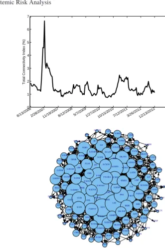
Fig. 1 Dynamics of total connectedness index over the period 2006-2012 obtained from a rolling estimation with windows size of 150-days.

0 1 2 3 4 5 6 7

Total Connectivity Index (%)

6/13/20062/28/200711/19/20078/12/20085/7/20091/27/201010/15/20107/12/20113/26/201212/13/2012

Fig. 2 Volatility network among the financial institu-tions for the period ending February 28, 2007. Size of the variable shows the degree of

connectedness in the network. I:BP

IAP I:G HSX LRE STJ I:US GPOR I:ISP G:ETE B:ACK ADM M:SAMA SGRO D:HN1X P:BCP O:ERS DK:JYS B:KB F:KN@F W:RTBF F:CNP PRU W:SEA EMG H:AGN AML F:SCO SHB INVP S:HEPN DK:TRY B:CofN D:DEQX S:PSPN I:PMI DLN D:DB1X LSE H:ING E:MAP N:STB O:IMMO G:PIST N:DNB O:RAI LGEN E:POP I:UBI W:INJ SDR F:MF@F F:GFC I:BMPS B:GBLN I:AZM DK:SYD III ICP S:PARG PFG O:WNST S:SPSN H:WH W:NDA W:SWED E:BSAB W:SVK DK:DAB D:CBKX HSBA G:PEIR HGG F:GARA F:LOI BKIR W:IU CGL W:KIVB S:CSGN S:GAM DK:TOP HMSO RBS BLND H:UBL E:BBVA INTU STAN BARC W:JMBF LLOY S:UBSN B:AGS D:ALVX OML S:SLHN CBG ADN E:SCH I:MB F:CRDA S:ZURN IGG H:VIB LAND AV. I:UCG RSA F:MIDI S:BALN W:CAST D:MU2X S:SREN W:ISBF F:SGE E:BKT F:BNP D:DBKX

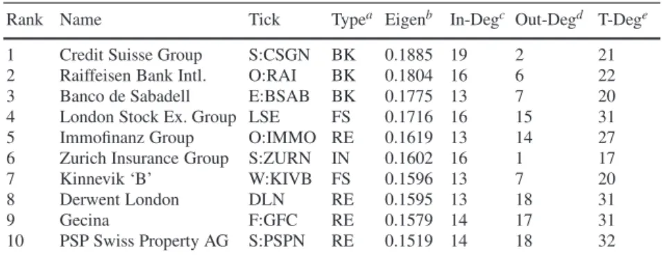
Estates in the Euro-area covering countries like Austria, Belgium, Finland, France, Germany, Greece, Ireland, Italy, Luxembourg, the Netherlands, Portugal, and Spain. We present the connectedness as the dependence pattern from a VAR(1) model with lag order based on testing the appropriate lag length using the BIC criteria and the available dataset (see [2]). We characterize the dynamics of the volatility con-nectedness (see Figure 1) using a rolling estimation with window size of 150-days over the sample period. From the figure, the highest total connectedness started early in the first quarter of 2007. We present in Figure 2, the graphical representation of the volatility network for the period ending February 28, 2007 which characterized the highest connectedness over the sample period. Table 1 report the top 10 institu-tions by eigenvector centrality from Figure 2. From the table, we observed that the top 10 central institutions as at the time was dominated by Banks, Financial Services and Real Estates. More specifically, we notice that prior to the global financial crisis between 2007-2009, the first quarter of 2007 shows evidence of some Banks, no-tably Credit Suisse Group in Switzerland, Raiffeisen Bank in Austria and Banco de Sabadell in Spain, acting as systemically important institutions in the “fear connect-edness” expressed by market participants in the financial sector of the Euro-area.

Table 1 Volatility Network Centrality Ranking

Rank Name Tick Typea _Eigenb _In-Degc _Out-Degd _T-Dege 1 Credit Suisse Group S:CSGN BK 0.1885 19 2 21 2 Raiffeisen Bank Intl. O:RAI BK 0.1804 16 6 22 3 Banco de Sabadell E:BSAB BK 0.1775 13 7 20 4 London Stock Ex. Group LSE FS 0.1716 16 15 31 5 Immofinanz Group O:IMMO RE 0.1619 13 14 27 6 Zurich Insurance Group S:ZURN IN 0.1602 16 1 17

7 Kinnevik ‘B’ W:KIVB FS 0.1596 13 7 20

8 Derwent London DLN RE 0.1595 13 18 31

9 Gecina F:GFC RE 0.1579 14 17 31

10 PSP Swiss Property AG S:PSPN RE 0.1519 14 18 32 Note: The table report the top 10 institutions by eigenvector centrality for the period ending February 28, 2007;a_{The financial super-sectors, BK (Banks), FS (Financial Services), RE (Real} Estates), and IN (Insurance);b_{Eigenvector Centrality;}c_In-Degree;d_Out-Degree;e_{Total Degree}

5 Conclusion

We applied sparse Bayesian graphical VAR model to the analysis of systemic risk on the European stock market. We found evidence of increased number of linkages between institutions during the 2007-2009 financial crisis. Our sparse method allows us to extract a reduced number of systemically relevant institutions with respect non-sparse approaches.

References

1. Ahelegbey D. F., Billio M, Casarin R.: Bayesian Graphical Models for Structural Vector Au-toregressive Processes. Journal of Applied Econometrics (forthcoming) (2015)

2. Alehegbey D. F., Billio, M. and Casarin, R.: Sparse Graphical Vector Autoregression: A Bayesian Approach, Working Paper N. 24/WP/2014, Dept. of Economics, University Ca’ Foscari of Venice (2014)

3. Diebold F., Yilmaz K.: On the Network Topology of Variance Decompositions: Measuring the Connectedness of Financial Firms. Journal of Econometrics 182(1): 119–134 (2014) 4. Donoho D.L.: High–Dimensional Centrally Symmetric Polytopes with Neighborliness

Pro-portional to Dimension. Discrete Computational Geometry 35: 617–652 (2006)

5. Geiger D., Heckerman D.: Parameter Priors for Directed Acyclic Graphical Models and the Characterization of Several Probability Distributions. Annals of Statistics 30: 2002 (1999). 6. Giudici P., Castelo R.: Improving Markov chain Monte Carlo Model Search For Data Mining.

Machine Learning 50: 127–158 (2003)

7. Lauritzen S. L., Wermuth N.: Graphical Models for Associations Between Variables, Some of Which Are Qualitative and Some Quantitative. Annals of Statistics 17: 31–57 (1989) 8. Scott J. G., Berger J. O.: Bayes and Empirical-Bayes Multiplicity Adjustment in the