Sample re-weighting hyper box classifier for multi-class data
classification
Lingjian Yang
a, Songsong Liu
a, Sophia Tsoka
b, Lazaros G. Papageorgiou
a,⇑ aCentre for Process Systems Engineering, Department of Chemical Engineering, University College London, Torrington Place, London WC1E 7JE, United Kingdom b
Department of Informatics, School of Natural and Mathematical Sciences, King’s College London, Strand, London WC2R 2LS, United Kingdom
a r t i c l e
i n f o
Article history:
Received 11 August 2014
Received in revised form 25 January 2015 Accepted 24 February 2015
Available online 9 March 2015 Keywords:
Multi-class data classification Mathematical programming Mixed integer optimisation Hyper box representation
a b s t r a c t
In this work, we propose two novel classifiers for multi-class classification problems using mathematical programming optimisation techniques. A hyper box-based classifier (Xu & Papageorgiou, 2009) that iteratively constructs hyper boxes to enclose samples of different classes has been adopted. We firstly propose a new solution procedure that updates the sample weights during each iteration, which tweaks the model to favour those difficult samples in the next iteration and therefore achieves a better final solu-tion. Through a number of real world data classification problems, we demonstrate that the proposed refined classifier results in consistently good classification performance, outperforming the original hyper box classifier and a number of other state-of-the-art classifiers.
Furthermore, we introduce a simple data space partition method to reduce the computational cost of the proposed sample re-weighting hyper box classifier. The partition method partitions the original data-set into two disjoint regions, followed by training sample re-weighting hyper box classifier for each region respectively. Through some real world datasets, we demonstrate the data space partition method considerably reduces the computational cost while maintaining the level of prediction accuracies. Ó2015 The Authors. Published by Elsevier Ltd. This is an open access article under the CC BY license (http://
creativecommons.org/licenses/by/4.0/).
1. Introduction
Given a set of samples, each of which is described by certain measurable features and labelled with a pre-determined class, data classification concerns identifying the pattern within the sample data and predicting the class labels of new samples. Data classifica-tion has a wide range of applicaclassifica-tions from financial analysis (Min & Lee, 2005; Sueyoshi, 2004; Sueyoshi & Goto, 2009), image classifi-cation (Chi, Feng, & Bruzzone, 2008; McCann & Lowe, 2012; Velasco-Forero & Angulo, 2013; Villa, Chanussot, Benediktsson, Jutten, & Dambreville, 2013), medical data for disease diagnosis or prognosis (Cascione, Ferro, Giugno, Pigola, & Pulvirenti, 2013; Dagliyan, Uney-Yuksektepe, Kavakli, & Turkay, 2011; Guyon, Weston, Barnihill, & Vapnik, 2002; Lee, Chuang, Kim, Ideker, & Lee, 2008; Seera & Lim, 2014; Su, Yoon, & Dougherty, 2009; Wei, Visweswaran, & Cooper, 2011; Yeoh et al., 2002), market price pre-diction (Anbazhagan & Kumarappan, 2012) and document classifi-cation (Li, Miao, & Wang, 2011; Sebastiani, 2002; Zhang & Gao, 2011).
Over the past decades, a wide range of classification algorithms have been proposed in literature to tackle various classification
problems. Classification algorithms can be broadly divided into two categories: binary and multi-class classifiers. A binary classi-fier is solely applicable to classification problems with two classes while a multi-class classifier can deal with problems with more than 2 classes. Compared with the large number of binary classi-fiers, there are relatively fewer multi-class classifiers in literature (Bal & Orkcu, 2011). Common strategies of tackling a multi-class classification problem include either solving the problem once using a multi-class classification algorithm or decomposing the whole problem into a series of binary problems and solving itera-tively the sub-problems using binary classifiers (Ou & Murphey, 2007; Wang, Chen, & Qin, 2010).
The existing classifiers in open literature are based on diverse methodologies, including support vector machine (SVM), neural network (NN), Naïve Bayesian, decision tree, mathematical pro-gramming optimisation techniques, and so on. We provide below a brief summary of some of the most popular classification approaches, with some key classifiers shown inFig. 1.
1.1. SVM
SVM constructs hyper plane to separate samples from different classes. SVM builds hyper plane with the maximum soft margin, i.e. maximising the margin between two classes while allowing
http://dx.doi.org/10.1016/j.cie.2015.02.022
0360-8352/Ó2015 The Authors. Published by Elsevier Ltd.
This is an open access article under the CC BY license (http://creativecommons.org/licenses/by/4.0/). ⇑Corresponding author. Tel.: +44 2076792563; fax: +44 2073882348.
E-mail addresses:[email protected](L. Yang),[email protected](S. Liu), [email protected](S. Tsoka),[email protected](L.G. Papageorgiou).
Contents lists available atScienceDirect
Computers & Industrial Engineering
j o u r n a l h o m e p a g e : w w w . e l s e v i e r . c o m / l o c a t e / c a i emisclassifications of the samples. The balance between distance of the constructed hyper plane to different classes of samples and the amount of misclassifications is controlled by a user-specified trade-off parameter. One of the features that make SVM powerful is the so-called kernel trick, which maps the dataset to higher-dimensional inner product space, at where samples may be easier to separate. A number of kernel functions, which greatly enhance the suitability of SVM in identifying non-linear decision bound-aries, can be employed, e.g., polynomial kernels and radial basis function kernel. Solving SVM has been formulated as a convex quadratic programming optimisation problem, which can be solved to global optimality using a large number of non-linear sol-vers (Carrizosa & Romero Morales, 2013; van Gestel et al., 2004). Despite the popularity, optimal tuning of the trade-off parameter and choice of kernel functions remain problem-specific issues that considerably affect the predictive power of SVM (Amari & Wu, 1999; Diosan, Rogozan, & Pecuchet, 2012; Noble, 2006; Ozer, Chen, & Cirpan, 2011).
1.2. NN
Mimicking a biological neural network, NN classifier consists of a number of connected layers of neurons, which transforms an input layer of features to an output layer of class labels. Each neuron takes input as weighted summation of outputs from all the neurons in the previous layer, and applies a non-linear activa-tion funcactiva-tion before passing the output to all the neurons in the next layer (Kavzoglu, 2009). Frequently used activation functions include: sigmoid, logarithmic and radial basis functions (Arulampalam & Bouzerdoum, 2003). Despite its capacity to tackle datasets with non-linear and complex decision boundaries, the number of hidden layers, how many neurons allowed for each hid-den layer, which activation function to use amount to a difficult optimisation problem, which limits the generality of the method (Hunter, Hao, Pukish, Kolbusz, & Wilamowski, 2012). In reality,
the structure of the network, i.e. the number of layers, the number of neurons for each layer and the types of activation function, are usually specified by the user, which reduces the problem of training a neural network classifier to tune the weights of connec-tions between consecutive layers of neurons to minimise the classification error. Training a neural network is known to be time consuming and can only guarantee local optimality.
1.3. Naïve Bayes
Naïve Bayes classifier belongs to the group of statistical classi-fiers. It is based on the naive assumption that the effect of different features on class membership predictions is independent from each other (Martinez-Arroyo & Sucar, 2000; Rish, 2001). In general, Naïve Bayes simply computes the support of each feature for each class so that the maximum likelihood estimate is satisfied in the training samples set. With the derived Bayesian rules the probabil-ity of a sample being predicted into a class can be calculated. The simplicity of Naïve Bayes classifiers also ensures computational efficiency (Almeida, Almeida, & Yamakami, 2011). Although the assumption of independence among features is more often than not violated in practical datasets, Naïve Bayesian generally gives comparable performance against much more sophisticated classi-fiers (Jin, Lu, & Ling, 2003; Rish, 2001; Wong, 2012).
1.4. Decision tree
Decision tree is a recursive partitioning method that sequen-tially splits samples into subsets. Starting from the whole dataset, decision tree identifies one attribute and a break point, before partitioning samples into subsets so that to improve the homogeneity of the class label vector within the subsets. The partitioning procedure is recurred for each child node until no fur-ther split can result in an increase in training sample accuracy (Chipman, George, & McCulloch, 1998; Gray & Fan, 2008). After
growing a large tree, small leaves that do not contribute signifi-cantly to the training accuracy are removed to improve the generalisation and predictive power of the constructed tree (Chipman et al., 1998; Polat & Gunes, 2007; Rastogi & Shim, 2000). Interpretability is one of the main strengths of decision tree classifier. The set of sequential linear rules generated are easy to understand, providing valuable insights into the mechanism of the underlying system. Decision tree has been shown to be particularly vulnerable that perturbing a small proportion of train-ing samples or re-sampltrain-ing the traintrain-ing set are likely to result in a very different tree structure (Gray & Fan, 2008).
1.5. Mathematical programming
Another group of classification models are built with mathe-matical programming optimisation techniques. Sueyoshi (1999, 2001, 2004, 2006), Sueyoshi and Goto (2009), Bal and Orkcu (2011) and Gehrlein (1986)have all proposed hyper planes-based classifiers using either linear programming or mixed integer pro-gramming techniques.Ryoo (2006)andBagirov, Ugon, and Webb (2011) propose models on piece-wise linear classifiers. In
Bertsimas and Shioda (2007), a model is presented separating sam-ples into a number of polyhedrons, which are formed by multiple hyper planes. The proposed formulation tries to enclose as many samples belonging to the same class into the same polyhedrons by optimising the positions of polyhedrons.
On the other hand,Xu and Papageorgiou (2006) and Xu and Papageorgiou (2009)produce a mathematical programming-based formulation modelling a hyper box (HB) classifier. A hyper box is essentially a multi-dimensional rectangle with the number of dimensions being equal to the total number of attributes in the dataset. The proposed method aims to build for each class a num-ber of hyper boxes enclosing as many samples as possible. The hyper boxes belonging to different classes are constrained to not overlap with each other, and each hyper box defines a distinct rule enclosing a proportion of training samples. InMaskooki (2013), a modified version of HB classifier has been developed which requires only 1/3–1/2 computational time compared with the original HB. Inspired by the promising performances of the HB classifier, we propose two refined hyper box classifiers in this work, aiming to improve the quality of the constructed boxes.
Many other classification algorithms based on mathematical programming optimisation techniques exist in literature but cannot be described here due to limited space (Armutlu, Ozdemir, Uney-Yuksektepe, Kavakli, & Turkay, 2008; Bal, orkcu, & Celebioglu, 2006; Bertsimas & Shioda, 2007; Glen, 2003; Kone & Karwan, 2011; Ma, 2012; Saigo, Nowozin, Kadowaki, Kudo, & Tsuda, 2009; Soylu & Akyol, 2014; Sun & Xiong, 2003; Turkay, Uney, & Yilmaz, 2005; Uney & Turkay, 2006; Xanthopoulos & Razzaghi, 2014; Zhang, Shi, & Zhang, 2009).
Without attempting to comprehensively review the above clas-sifiers, we summarise their relative strengths and weaknesses in
Table 1below.
1.6. Ensemble classifiers
Besides the single classifiers described above, some recent research efforts have been focusing on developing ensemble classi-fiers, which builds a number of single classifiers and aggregate their classification outcomes to produce the final prediction (Breiman, 1996). Given a training sample set, Bagging (Bauer & Kohavi, 1999; Rokach, 2009) creates a number of bootstrap sample sets by uniformly sampling with replacements, and each bootstrap sam-ple set is then learned by a classifier. The final prediction is an aggregation of decisions made by each classifier, by simple average or more sophisticated voting strategy that certain classifiers have
more votes in the final decision (Breiman, 1996; Strobl, Malley, & Tutz, 2009). Another recent advance in ensemble classification algorithm is Boosting (Niu, Jin, Lu, & Li, 2009). One of the most recognised Boosting algorithms is Adaboost (Freund & Schapire, 1997), which trains a set of classifiers in an iterative manner so that the subsequent classifiers are constructed in favour of those sam-ples misclassified by the last classifier, by updating the weights of samples. Given a new sample with unknown class label, all the sin-gle classifiers make their own predictions of which class it belongs to and their decisions are combined to yield a final prediction.
In this work, we introduce two new solution procedures to improve the performance of the HB classifier. We firstly extend our previous work of HB classifier by incorporating a sample re-weighting scheme. For HB classifier, misclassified samples can either be outside all the derived hype boxes or can be enclosed in hyper boxes belonging to other classes. Our proposed sample re-weighting scheme works by assigning higher weights to mis-classified samples enclosed by other hyper boxes, tweaking the model to favour those difficult samples in the next iteration. In doing so, we aim to increase the chance of them being correctly classified in subsequent iteration and achieving a better final solu-tion. Furthermore, observing the generally high computational cost of the traditional HB classifier, we have introduced a data space splitting method that partitions the training samples into two dis-joint regions, each one of which defines a much smaller optimisa-tion problem and thus can be solved easier. Computaoptimisa-tional experiments clearly demonstrate that the proposed sample re-weighting scheme achieves consistently higher prediction accuracy than the traditional HB classifier. Meanwhile, the sample partitioning method reduces the computational cost by 1 or 2 orders of magnitudes on the basis of maintaining the desirable level of prediction rates.
The rest of the paper is structured as follows: in Section2, we will summarise both mathematical formulation and solution procedure of the original HB classifier (Xu & Papageorgiou, 2006, 2009), which also serves as the basis of our work. Section3 pro-poses a refined HB classifier. In Section4we further introduce a data space partition method in a bid to ease the high com-putational demand of constructing hyper box classifier. Results of computational experiments on a number of real world datasets are to appear in Section5, with the last section concludes with our major findings.
2. A hyper box classifier
As mentioned before, our work is based on the classification method proposed in Xu and Papageorgiou (2006, 2009), which
Table 1
Relative strength and weakness of certain classifiers.
Strength Weakness
SVM Guarantee of global
optimality; use of kernel function to map the original data to higher dimensional feature space
User specified kernel functions; user specified tuning parameters; lack of interpretability
NN Flexible to learn any
functional relationship
User specified network structures; user specified activation functions; lack of interpretability
Naïve Bayes Simplicity Often unrealistic statistical assumption
Decision tree Good interpretability; little computational time
Tree structure sensitive to slight change in training samples
Hyper box Free of tuning parameters; good interpretability
High computational cost due to its use of integer programming
describes a mathematical programming formulation modelling classification boundaries as multiple high dimensional rectangles. We summarise below the original formulation before presenting our proposed refinements.
2.1. Mathematical model of HB
The indices, parameters and variables associated with the model are listed below:
Indices
s sample
m attribute
i,j hyper box
is hyper boxithat samplesis mapped into
c,k class
ic hyper boxithat belongs to classc
Parameters
Asm numeric value of sampleson attributem C the total number of classes
M the total number of attributes
U a large positive number
e
a small positive number Continuos variableXim central coordinate of hyper boxion attributem LEim length of hyper boxion attributem
Binary variable
Es 1if samplesis correctly enclosed in its hyper boxis;0
otherwise
Yijm 1if on attributemlower bound of hyper boxiis greater than upper bound of hyper boxjand ensuring non-overlapping between the two;0otherwise
Whether a samplesis enclosed in its corresponding hyper boxi
or not is modelled using the following two sets of constraints:
AsmPXimLEim
2 U ð1EsÞ
8
s;is;m ð1ÞAsm6XimþLEim
2 þU ð1EsÞ
8
s;is;m ð2ÞIfEstakes the value of1, samplesis correctly enclosed in hyper box
is, i.e. value ofAsmlies between the lower bound (XimLEim/2) and
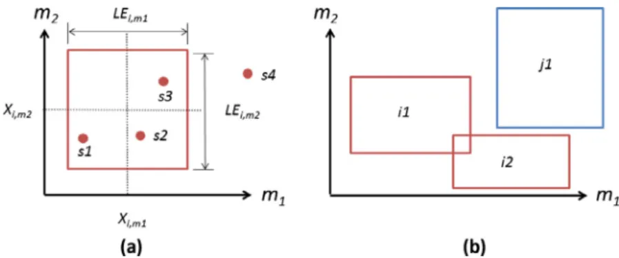
upper bound (Xim+LEim/2) of its hyper box is for all attributes; otherwise samplesis misclassified as being outside its target box. InFig. 2a, we present a two dimensional presentation of samples being inside and outside their corresponding hyper boxes. Hyper boxes of different classes are not allowed to overlap, which is rea-lised via the following two sets of constraints:
XimXjmþUYijmPLEimþLEjm
2 þ
e
8
m;ic;jk;c–k ð3Þ XmðYijmþYjimÞ62M1
8
ic;jk;c<k ð4ÞIn constraint(3), when binary variableYijm= 0, hyper box iandj
belonging to different classes do not overlap, i.e. lower bound of boxiis greater than upper bound of boxjon attributem;when bin-ary variableYijm= 1 constraints (3) become redundant. To avoid overlapping of the hyper boxes inM-dimensional space, they need to not overlap in at least one dimension, which is modelled by con-straints(4). InFig. 2b, we give a graphical example of overlapping and non-overlapping hyper boxes. The objective function is to min-imise the number of misclassifications (i.e.Es=0):
minX
s
ð1EsÞ ð5Þ
Objective function (5), sample enclosing constraints(1), (2), and hyper box non-overlapping constraints (3), (4)form the original mathematical formulation, named MCP, in the original HB classifier (Xu & Papageorgiou, 2009). The combination of linear objective function and linear constraints, and presence of binary variables define a mixed integer linear programming (MILP) formulation, which can be solved to global optimality using standard solution techniques, for example branch-and-bound.
2.2. HB iterative solution procedure
Last section describes a mathematical programming formula-tion for building hyper boxes to separate samples. In Xu and Papageorgiou (2009), an iterative solution procedure has also been developed to allow potentially multiple hyper boxes per class to improve the quality of the solution. This old iterative procedure is outlined inFig. 3below.
Initially, one hyper box is created for each class of samples (ini-tialiseis) and the MCP model is solved once to enclose as many as possible the samples into their own hyper boxes. Starting from the second iteration, for any class having at least one misclassified sample (Es=0), one additional hyper box is allowed for this particular class, followed by updatingis, i.e. the correct classified
samples are still mapped to their original hyper box while the misclassified samples are re-mapped to the new box. For the classes that all their samples are correctly classified in the last iteration, their sample-box mappingisare kept. The iterative pro-cedure terminates when the number of misclassified samples does not decrease in two adjacent iterations or when all the samples are correctly classified. An artificial example is given in Fig. 4 to illustrate the old iterative solution procedure.
2.3. Predicting new samples using derived hyper boxes
After training the HB classifier the derived hyper boxes are used to predict the class label of a new sample. The prediction procedure is intuitive as: (1) if a new sample falls into one of the derived boxes, it is assigned the class label of the box; (2) if a new samples lies outside all derived hyper boxes, it is assigned the class label of its nearest box.
After reviewing the main features of hyper box classifier pro-posed byXu and Papageorgiou (2009), we are going to propose a refined HB classifier in the next section.
3. A refined hyper box classifier
Inspired by the success of boosting algorithms, which typically consists of iteratively learning classifiers while updating the weight distribution of samples, we have introduced a sample reweighting scheme into the traditional hyper box classifier in a bid to improve its performance.
As mentioned earlier in Section2, the traditional HB inherently involves iterative training, i.e., after each iteration any class with misclassified samples is updated with an extra hyper box and the MCP model is re-solved. In our proposed work, we mimic the beha-viour of boosting algorithms by reweighting samples between iterations. More specifically, after each iteration, we update the weights of all samples by assigning more weights to a subset of misclassified samples, thus putting more emphasis into correctly classifying them in the next iteration. When a sample s is mis-classified by its hyper box, the misclassification can fall into two categories: (1) misclassified sample lies outside all derived boxes; (2) misclassified sample lies inside at least one of the derived boxes
that belong to a different class. We call the two types of errors type1 and type 2, respectively.Fig. 5visualises the two types of misclassifications for a two dimensional case.
InFig. 5a, two misclassified samples lie outside both derived hyper boxes and before the next iteration, another box will be allo-cated for the two samples of type 1 error. In the second iteration, the two samples will be correctly enclosed in the additional hyper box. InFig. 5b, however, the two type 2 misclassified samples will still be misclassified in the next iteration despite another allocated hyper box. In fact, type 2 misclassified samples have only slight chance of being correctly classified in the following iterations. In this work, we propose a sample re-weighting scheme that gives more weights to the type 2 misclassifications, which then will
increase the chance of them being correctly classified and achiev-ing a better final solution. In order to accommodate the different weights of samples, the objective function(5) in the traditional HB has been modified to the following:
minX
s
Psð1EsÞ ð6Þ
wherePsdenote the weight of samples, equivalent to the cost of misclassification. Eq.(5)can be seen as a special case of Eq. (6)
wherePs= 1 for all samples. Considering the new objective function, when different weights are assigned to different samples, the model will prioritise those samples with higher weights for the overall misclassification cost to reach globally minimum. We keep other
Fig. 2.Graphic explanations of mathematical formulation of HB. a: samples1,s2 ands3 are correctly enclosed in its hyper box (i.e.Es= 1) while samples4 lies outside the box
(i.e.Es= 0); b: hyper box non-overlapping constraints(3) and (4)ensure that hyper boxes belonging to different classes (i1–j1 andi2–j1) cannot overlap while the restriction
does not apply to boxes belonging to the same class (i1–i2). Boxesi1–j1 are non-overlapping because they do not overlap on attributem1 (i.e.Yj1,i1,m1= 0), whilei2–j1 do not overlap on attributem2 (i.e.Yj1,i2,m2= 0).
constraints(1)–(4)in the new formulation, which is named W_MCP (Weighting_MCP). The W_MCP formulation is still an MILP. The flowchart of the modified iterative hyper box method, called SRW_HB (Sample Re-Weighting_Hyper Box), is constructed in
Fig. 6.
The proposed SRW_HB also implements an iterative solution procedure. The first iteration of SRW_HB is identical to the first iteration of the traditional HB that one box per class is generated to minimise the total cost of misclassifications while all the sam-ples are having a weight value,Ps, of1. If there are misclassified samples, from the second iteration one more box is allowed for each class with at least one misclassified sample. The sample-box mapping is updated that correctly classified samples from the last iteration keep their mapping from the last iteration, while the mis-classified samples (both type 1 and type 2) are re-mapped to their newly generated hyper boxes. The misclassification cost for cor-rectly classified samples and type 1 misclassified samples are set
to1, while the cost for type 2 misclassified samples are set to a higher valueCT(CT > 1). The W_MCP model is re-solved and the above procedure is repeated. The iterative solution procedure ter-minates when the number of misclassified samples fail to improve in 2 consecutive iterations. The testing procedure is the same as the original HB that a new sample is allocated to its nearest derived hyper box and then assigned the membership of the hyper box.
4. A data space partition scheme
In the original publication (Xu & Papageorgiou, 2009), it is claimed that for some datasets, MCP models cannot be solved to global optimality in 200s for all iterations. Note that computational complexity of an MILP problem is dependent on the size of the problem, we therefore propose here a simple data space partition scheme to ease the computational burden of building hyper boxes and attempt to identify better solutions.
Given a datasetAsm, the average value of all samples on each attributemis calculated asAverm, followed by computing the num-ber of samples satisfying AsmPAverm and Asm<Averm, respec-tively, which are denoted as RUm and RLm. Compute for each attribute the difference between the samples placed in the two dis-joint regions partitioned from Averm as Diffm= |RUmRLm|. The attribute offering the most even partition, i.e. the smallest Diffm
value is selected as the partition attributem⁄. When there are
mul-tiple attributes offering equally lowDiffmvalue, the partition attri-bute is randomly chosen among them. Subsequently the original dataset is partitioned into two disjoint regions R1 and R2, which respectively contain samples satisfying AsmPA
v
erm and Asm<Av
erm. In each region, we train the proposed samplere-weighting hyper box classifier (SRW_HB). It is important to note that extra constraints are added to the W_MCP to make sure that the derived hyper boxes from each region are not unnecessarily large to overlap with hyper boxes derived from the other region on the partition attributem⁄, thus ensuring the boxes in one region
do not overlap with the boxes in the other region:
XimLEim 2 PA
v
erm8
i;m¼m ð7Þ XimþLEim 2 6Av
erme
8
i;m¼m ð8ÞEq. (7) are added to W_MCP when solving R1 while Eq. (8)are added to W_MCP when training on samples in R2. An arbitrarily small positive constant
e
is inserted in Eq.(8)to ensure the two regions do not share the same boundary. The final decision bound-ary is formed by all the derived hyper boxes from both regions. The idea behind the data space partition method is that the required computational time to solve an MILP grows exponentially with the number of training samples, making it hard to identify optimal solutions at feasible computational cost. Partition the dataset intoFig. 4.HB iterative solution procedure. At the initial iteration one box is allowed per class and after solving the MCP model, the 4 misclassified samples represented by circles are re-assigned to an extra box while no additional box is given to the class represented by triangle due to zero misclassifications. After solving the MCP model for the 2nd iteration, the only misclassified sample from the circle class is given another box, followed by solving the MCP model another time. The iterative procedure terminates at the 3rd iteration because the total number of mis-classifications fails to decrease from the last iteration.
Fig. 5.Two types of hyper box misclassifications. a: Type 1 misclassification that samples are not enclosed correctly by its hyper box and are outside all the boxes from other classes; b: type 2 misclassification that samples are not enclosed correctly by its hyper box and are inside at least one of the boxes belonging to another class.
two disjoint regions with similar numbers of samples makes both regions equally easy to solve. We name the framework employing the proposed simple data space partition scheme to create two dis-joint sub-regions and construct sample re-weighting hyper box classifiers in both regions as DR_SRW_HB, the flowchart of which is illustrated inFig. 7.
In this work we have tested the proposed data space partition scheme, which splits the entire data space into two disjoint regions, on medium-size datasets. It is important to note that for larger size datasets, the current proposed strategy can be further generalised, i.e., partition the data space into 3, 4 or more disjoint parts, to accommodate more samples and attributes.
5. Computational results
In this section, the applicability and effectiveness of the pro-posed SRW_HB and DR_SRW_HB classifiers are demonstrated through 6 real world datasets, including Phenol (Niu et al., 2009), Firm (Sueyoshi, 2006; Xu & Papageorgiou, 2009) and 4 datasets downloaded from UCI machine learning repository (http:// archive.ics.uci.edu/ml/), namely Ionosphere, glass, breast tissue, and iris. We have implemented a number of literature classifiers to compare the classification rates with our proposed SRW_HB and DR_SRW_HB. The group of classifiers include Naïve Bayes, SMO (support vector machine), Logistic regression, Bagging, Adaboost, NN and three mathematical programming-based multi-class multi-classifiers: HB,Gehrlein (1986)andBal and Orkcu (2011).
To comprehensively evaluate the overall classification perfor-mances of various classification algorithms, we use two testing scenarios as below:
Scenario 1:perform 50 random partitions of each dataset into a training set containing 70% samples and a testing set containing the 30% samples. For each partition we train a classifier on training set and test the classification performance on testing set.
Scenario 2: conduct a leave-one-out cross validation that for each dataset hold only one sample in the testing set while using the rest as training samples. The process is repeated until all sam-ples are used as testing sample.
All the mathematical programming-based classification meth-ods, including SRW_HB, HB, and approaches proposed by
Gehrlein (1986)and Bal and Orkcu (2011), are implemented in General Algebraic Modeling System (GAMS) 24.1 (GAMS Development Corporation, 2013) and solved using CPLEX 12.3 sol-ver on a 2.40 GHz speed, 2393 MHz cpu computer system. Optimality gap is set as 0 when solving MILP problems. For all hyper box-based methods we limit the computational time per iteration as 200 s. Other classifiers are implemented in Waikato Environment for Knowledge Analysis (WEKA) machine learning software (Hall et al., 2009). Default setting are retained for Naïve Bayes, Logistic regression, SMO, Bagging and Adaboost, while for NN the following parameters fromXu and Papageorgiou (2009)
are used: hidenLayers = 2; learning rate = 0.1; momentum = 0.7; trainingTime = 10,000.
5.1. Real world datasets
We use 6 real world datasets to test the applicability and com-petitiveness of the proposed classification algorithms. Ionosphere concerns some radar data that given 34 attributes reflecting the received signals the task is to classify free electrons in the
Fig. 6.Flowchart of the proposed SRW_HB. The highlighted content in red differentiates the SRW_HB from the traditional HB. (For interpretation of the references to colour in this figure legend, the reader is referred to the web version of this article.)
ionosphere into 2 classes. The dataset Phenol (Niu et al., 2009) con-cerns classifying 274 phenols, characterised by 9 molecular descriptors that quantify their compounds, into 4 possible toxicity mechanisms including polar narcotics, respiratory uncouplers, pro-electrophiles and soft pro-electrophiles. Glass example downloaded is a collection of glass samples belonging to 6 types of glass. Each glass sample is descripted by 9 attributes, each of which corresponds to weight percentage of a chemical compound (sodium, aluminium, calcium, etc.) in corresponding oxide. Breast tissue dataset has 106 freshly excised tissue samples in the breast area, and are descripted by 9 attributes such as area under spectrum, length of the spectral curve. Iris is one of the most studied benchmark data-sets in data classification. 150 instances from 3 types of iris plant are characterised by 4 features, including sepal length, sepal width, petal length and petal width. Firm dataset aims to predict the financial performance of a number of companies, based on certain performance indices for example cash to total assets, long-term debt to total assets, into a class of ‘good’ firms and the other class of firms went bankrupt between 1996 and 2002. A brief summary of the employed real world datasets is provided inTable 2.
5.2. Sensitivity analysis of CT
In this section, a sensitivity analysis is performed to tune the user-specific parameter CT for the proposed SRW_HB, which denotes the cost for type 2 misclassified samples and is higher than 1. We present inFig. 8the results of sensitivity analysis for all the 6 datasets.
A series of values have been tested forCT, including 2, 3, 4 and 5. It is clear fromFig. 8that varyingCThas different effects on differ-ent datasets. For Ionosphere dataset and scenario 1, prediction accuracy first increases fromCT =2 toCT =3, and then falls down whenCTis equal to 4 and 5. With regards to scenario 2, the trend is similar that prediction rate goes up fromCT =2 toCT =3, and then decreases later on. For Phenol, asCTincreases classification
rate for scenario 2 goes up from CT =2 to CT =3, 4 before decreasing when CT =5, while classification rates for scenario 1 keep constant. Glass is the mostly affected by different values of
CT among all tested datasets that for both scenarios prediction rates increase fromCT =2 to 4 by about 5%, which subsequently drops down whenCT =5. With regards to Breast tissue case study, classification rates for both scenarios fluctuate throughout the testedCTvalues and both peaked atCT =3. When it comes to Iris dataset, increasingCTappears to have minor impact on scenario 1 while for scenario 2 prediction rate keeps constant between
CT =2 and 4 before growing slightly withCT =5. Lastly, for Firm dataset, classification rate for scenario 2 keeps constant over the tested range while for scenario 1 the accuracy goes down from
CT =4 to 5.
Overall, it is obvious that the sensitivity analysis for SRW_HB does not yield a clear optimal CT value, as in different datasets and different scenarios peak prediction rates come from different
CTvalues. On the other hand, it appears thatCT =3 gives a robust performance as prediction rate often peaks at or nearCT =3 (e.g. Ionosphere, Breast Tissue). Therefore we take CT =3 for SRW_HB when comparing its classification performance against other implemented classifiers in literature, which has good performance for almost all datasets investigated.
Fig. 7.Flowchart of the proposed DR_SRW_HB.
Table 2
Summary of real world datasets. Dataset Number of samples Number of attributes Number of classes Ionosphere 351 34 2 Phenol 274 9 4 Glass 214 9 6 Breast tissue 106 9 6 Iris 150 4 3 Firm 83 13 2
5.3. Classification performance comparison
In this section, we evaluate the classification performance of 10 classifiers, including the proposed SRW_HB and traditional HB. For the proposed SRW_HB classifier, we setCT =3 for all datasets to offer a fair comparison. The results are presented inTables 3 and 4for scenario 1 and 2, respectively.
For both testing scenarios, no classifiers are showing dominant classification rates against others, as different datasets play to the strengths of different classification methodologies. This observa-tion is consistent with the previous findings (Adem & Gochet, 2006; Lam & Moy, 2002). A good classifier should maintain consis-tently good performance across many different classification prob-lems. The proposed SRW_HB, showing this desired consistency, is usually among the top 3 out of the 10 classifiers. Note that the pro-posed SRW_HB outperforms the traditional HB for most scenarios. We summarise here the overall classification performance of the 10 implemented classifiers by using a scoring scheme, employed also inXu and Papageorgiou (2009). Briefly, for each sce-nario and a particular dataset, the classifiers are ranked in descend-ing order accorddescend-ing to their prediction accuracies, i.e. the classifier with the highest classification rate is awarded a score of 10; the classifier with the second highest classification rate is assigned a score of 9, and so on. For each scenario, the average score across all datasets is taken as the indication of the overall competitiveness
of a particular classifier. The higher the average score, the better the performance of the classifier.
The score ranking is presented inFig. 9, which shows that in both scenarios the proposed SRW_HB classifier not only gives improved classification accuracy from the traditional HB, but also outperforms other state-of-the-art classifiers.
5.4. DR_SRW_HB significantly reduces computational cost while maintaining the classification accuracy compared with SRW_HB
In the last section, we demonstrate that the proposed SRW_HB classifier, which modifies the traditional HB classifier by updating the misclassification costs for samples with type 2 errors after each iteration, gives overall better prediction accuracy compared with a number of state-of-the-art classifiers. Recall that we have proposed in Section4a DR_SRW_HB method that implements a simple data space partition scheme to split the original data space into two dis-join regions, followed by training the SRW_HB for both regions. The idea is that each region contains about half samples of the entire problem, which is then much easier to solve.
We now test the effectiveness of the DR_SRW_HB against SRW_HB for both scenarios. With regard to the proposed SRW_HB method, W_MCP model cannot be solved to global optimality for at least one iteration (within 200 s) on 4 datasets (either scenario), including Phenol, Glass, Breast tissue and
Fig. 8.Sensitivity analysis ofCTfor the proposed SRW_HB on two testing scenarios. Blue line with triangle markers denotes scenario 1 and red line with round markers denotes scenario 2. (For interpretation of the references to colour in this figure legend, the reader is referred to the web version of this article.)
Ionosphere. We therefore run DR_SRW_HB on those 4 datasets and compare the prediction accuracy with that achieved by SRW_HB. The results are presented inTable 5. For scenario 1, DR_SRW_HB leads to higher classification rate on Phenol while SRW_HB is more accurate on Glass, Breast tissue and Ionosphere. It should be noted that compared other literature classifiers, DR_SRW_HB still shows better overall performance. When it comes to scenario 2, DR_SRW_HB offers much higher prediction rates on Glass example, ties with SRW_HB on Phenol and Breast Tissue while losing on Ionosphere example. We can see that DR_SRW_HB performs better in scenario 2 than scenario 1, because scenario 2 requires more computational effort than scenario 1 as a result of more samples involved in training of scenario 2. Considering both two scenarios, it is therefore conclusive that the proposed data space partition scheme can maintain the overall prediction rates of SRW_HB on complex examples.
Recall that the DR_SRW_HB has been proposed to overcome the high computational cost of tackling complex classification prob-lems, we report here, for scenario 2, the average computational
Table 3
Classification rate comparison for scenario 1.
Classifiers/dataset Ionosphere (%) Phenol (%) Glass (%) Breast tissue (%) Iris (%) Firm (%)
SRW_HB 90.69 89.41 71.09 66.32 95.64 93.84
HB 89.37 87.02 68.53 63.16 94.76 93.92
Gehrlein (1986) 84.55 86.05 56.68 52.32 93.64 86.67
Bal and Orkcu (2011) 89.15 84.80 61.59 59.23 86.93 89.20
Naïve Bayesian 82.52 86.29 48.13 67.34 96.00 92.61 SMO 87.94 81.29 55.84 54.31 96.67 93.16 Logistic regression 86.48 88.07 62.16 64.56 95.56 86.73 Bagging 90.96 90.17 68.69 66.75 94.67 92.43 Adaboost 90.36 77.85 42.78 36.19 94.36 93.16 NN 88.77 87.99 59.97 60.66 95.11 93.23
For each dataset, the highest classification accuracy achieved is marked in bold.
Table 4
Classification rate comparison for scenario 2.
Classifiers/dataset Ionosphere (%) Phenol (%) Glass (%) Breast tissue (%) Iris (%) Firm (%)
SRW_HB 91.17 92.34 66.36 67.92 96.00 95.18
HB 89.74 90.51 65.89 66.98 94.00 95.18
Gehrlein (1986) 85.47 85.77 56.07 64.15 94.00 81.93
Bal and Orkcu (2011) 87.18 87.59 64.95 68.87 88.67 98.80
Naïve Bayesian 82.62 86.50 49.53 66.04 95.33 91.57 SMO 88.03 79.56 54.67 56.60 96.67 95.18 Logistic regression 89.17 89.05 62.62 68.87 98.00 84.34 Bagging 92.02 91.24 72.90 65.09 94.00 90.36 Adaboost 90.88 78.47 44.86 40.57 97.33 93.98 NN 89.46 88.69 59.35 60.38 95.33 91.57
For each dataset, the highest classification accuracy achieved is marked in bold.
Fig. 9.Overall standing of classifiers. We give scores to competing classifiers according to the ranking of their classification rates in each dataset and average the scores over all dataset to comprehensively evaluate their relative competitiveness. In both scenarios, the proposed SRW_HB leads to the most robust classification performance across all implemented classifiers.
Table 5
Classification rate comparison between two proposed classifiers DR_SRW_HB and SRW_HB.
Ionosphere (%) Phenol (%) Glass (%) Breast tissue (%) Scenario 1 DR_SRW_HB 90.08 90.41 69.19 63.55 SRW_HB 90.69 89.41 71.09 66.32 Scenario 2 DR_SRW_HB 89.74 92.34 73.36 67.92 SRW_HB 91.17 92.34 66.36 67.92
time per run consumed by three variants of hyper box-based classifiers, namely HB, SRW_HB and DR_SRW_HB. The results, presented inFig. 10, show clearly that by partitioning a complex problem into two sub-problems and solving two relatively easy problems, the computational cost dramatically decreases. On Phenol and Breast tissue, DR_SRW_HB constructs hyper boxes in a matter of seconds while the CPU time consumed by HB and SRW_HB are significantly higher. While it takes hundreds of sec-onds for DR_SRW_HB to train hyper boxes on Glass and Ionosphere, the actual computational time is still small fractions of the consumption of HB and SRW_HB. For scenario 1, the trend is similar that the proposed data space partition method con-siderably reduces computational cost (data not shown). We also compare our proposed DR_SRW_HB with an alternative solution procedure proposed in literature for hyper box classifier (Maskooki, 2013), in which after each iteration, correctly classified training samples are removed and the dimensions of established hyper boxes are fixed before optimising the hyper boxes for the next iteration. It has been shown that the proposed solution proce-dure results in the computational cost saving of 2–3-fold and gen-erally decreased classification accuracy. Our proposed DR_SRW_HB classifier clearly outperforms (Maskooki, 2013) by offering much higher computational cost reduction. Thus, it is concluded that DR_SRW_HB results in huge CPU savings of 1 or 2 orders of magni-tude, compared with HB and SRW_HB. Overall, we propose here a strategy that for a classification problem which SRW_HB struggles to identify globally optimal solutions for all iterations, the DR_SRW_HB is used instead; otherwise for an easy classification problem, the SRW_HB is used.
Despite the significant reduction in computational time, DR_SRW_HB, based on mixed integer programming, is still gener-ally consuming more computational resource than the existing methods in literature. We note here that the prediction accuracy remains the most important aspect of many real world data classi-fication problems, for example medical disease classiclassi-fication prob-lems (Dagliyan et al., 2011; Nguyen & Rocke, 2002; West et al., 2001). The classifiers proposed in this work are aimed to achieve
higher prediction accuracy for offline classification problems where computational time is not of major concern.
6. Concluding remarks
Data classification is an important data mining area subject to extensive on-going research interest. Inspired by the promising classification rates of a hyper box classifier (Xu & Papageorgiou, 2006, 2009) in literature, we propose in this work two new solu-tion procedures that aim to improve the performance of hyper box classifier. The first improvement, SRW_HB, updates the sam-ples weights during each iteration of the training process so that the type 2 misclassified samples, i.e. misclassified samples enclosed in one of the hyper boxes from another class, are given more weights than the other samples. Through 6 binary and multi-class real world datasets, it is demonstrated that the pro-posed SRW_HB can provide consistently good classification rates, outperforming the traditional HB and other state-of-the-art classi-fiers for example SVM, NN and Logistic regression.
We further introduce a data space partition method to reduce the computational cost of SRW_HB, which works by splitting the data-set into two disjoint regions, each of which is then solved indepen-dently using SRW_HB. On the 4 complex datasets, the proposed DR_SRW_HB appears to consume dramatically less computational time than the original HB and SRW_HB, often in 1 to 2 orders of mag-nitude, on the basis of maintaining the desirable level of prediction accuracy compared with the proposed SRW_HB classifier.
A natural extension of this work in the near future is to investi-gate a more generic data space partition scheme. The sample partition scheme presented and used for DR_SRW_HB proves to significantly reduce computational cost but can only perform binary partition. For large-scale data classification problems, the proposed DR_SRW_HB may struggle to identify quality solution in training procedure. Therefore, a generic data space partition method, which splits data into multiple regions and each one of which is easy to solve, can help scale up the hyper box classifiers to large-size problems.
Fig. 10.Computational cost comparison between HB, SRW_HB and DR_SRW_HB. In the figure, average computational time per run of scenario 2 is reported for traditional HB, SRW_HB and DR_SRW_HB on 4 datasets Phenol, Glass, Breast tissue and Ionosphere. It is obvious that the DR_SRW_HB, which solves two sub-problems of smaller sizes, requires significantly lower computational cost.
Acknowledgments
Funding from the UK Engineering and Physical Sciences Research Council (to LY, SL and LGP for the EPSRC Centre for Innovative Manufacturing in Emergent Macromolecular Therapies), the UK Leverhulme Trust (to ST and LGP, RPG-2012-686) and the European Union (to ST, HEALTH-F2-2011-261366) is gratefully acknowledged.
References
Adem, J., & Gochet, W. (2006). Mathematical programming based heuristics for improving LP-generated classifiers for the multiclass supervised classification problem.European Journal of Operational Research, 168, 181–199.
Almeida, T., Almeida, J., & Yamakami, A. (2011). Spam filtering: How the dimensionality reduction affects the accuracy of Naive Bayes classifiers. Journal of Internet Services and Applications, 1, 183–200.
Amari, S., & Wu, S. (1999). Improving support vector machine classifiers by modifying kernel functions.Neural Networks, 12, 783–789.
Anbazhagan, S., & Kumarappan, N. (2012). A neural network approach to day-ahead deregulated electricity market prices classification. Electric Power Systems Research, 86, 140–150.
Armutlu, P., Ozdemir, M., Uney-Yuksektepe, F., Kavakli, I. H., & Turkay, M. (2008). Classification of drug molecules considering their IC50 values using mixed-integer linear programming based hyper-boxes method.BMC Bioinformatics, 9, 411.
Arulampalam, G., & Bouzerdoum, A. (2003). A generalized feedforward neural network architecture for classification and regression.Neural Networks, 16, 561–568.
Bagirov, A. M., Ugon, J., & Webb, D. (2011). An efficient algorithm for the incremental construction of a piecewise linear classifier.Information Systems, 36, 782–790.
Bal, H., & Orkcu, H. H. (2011). A new mathematical programming approach to multi-group classification problems.Computers & Operations Research, 38, 105–111. Bal, H., orkcu, H. H., & Celebioglu, S. (2006). An experimental comparison of the new
goal programming and the linear programming approaches in the two-group discriminant problems.Computers & Industrial Engineering, 50, 296–311. Bauer, E., & Kohavi, R. (1999). An empirical comparison of voting classification
algorithms: Bagging, boosting, and variants.Machine Learning, 36, 105–139. Bertsimas, D., & Shioda, R. (2007). Classification and regression via integer
optimization.Operations Research, 55, 252–271.
Breiman, L. (1996). Bagging predictors.Machine Learning, 24, 123–140.
Carrizosa, E., & Romero Morales, D. (2013). Supervised classification and mathematical optimization.Computers & Operations Research, 40, 150–165. Cascione, L., Ferro, A., Giugno, R., Pigola, G., & Pulvirenti, A. (2013). Microarray data
analysis: From preparation to classification. InBiological knowledge discovery handbook(pp. 657–674). John Wiley & Sons, Inc.
Chi, M., Feng, R., & Bruzzone, L. (2008). Classification of hyperspectral remote-sensing data with primal SVM for small-sized training dataset problem. Advances in Space Research, 41, 1793–1799.
Chipman, H. A., George, E. I., & McCulloch, R. E. (1998). Bayesian CART model search. Journal of the American Statistical Association, 93, 935–948.
Dagliyan, O., Uney-Yuksektepe, F., Kavakli, I. H., & Turkay, M. (2011). Optimization based tumor classification from microarray gene expression data.PLoS One, 6, e14579.
Diosan, L., Rogozan, A., & Pecuchet, J. P. (2012). Improving classification performance of support vector machine by genetically optimising kernel shape and hyper-parameters.Applied Intelligence, 36, 280–294.
Freund, Y., & Schapire, R. E. (1997). A decision-theoretic generalization of on-line learning and an application to boosting.Journal of Computer and System Sciences, 55, 119–139.
GAMS Development Corporation (2013).General algebraic modeling system (GAMS) release 24.2.1. Washington, DC, USA.
Gehrlein, W. V. (1986). General mathematical-programming formulations for the statistical classification problem.Operations Research Letters, 5, 299–304. Glen, J. J. (2003). An iterative mixed integer programming method for classification
accuracy maximizing discriminant analysis.Computers & Operations Research, 30, 181–198.
Gray, J. B., & Fan, G. (2008). Classification tree analysis using TARGET.Computational Statistics & Data Analysis, 52, 1362–1372.
Guyon, I., Weston, J., Barnihill, S., & Vapnik, V. (2002). Gene selection for cancer classification using support vector machines.Machine Learning, 46, 389–422. Hall, M., Frank, E., Holms, G., Pfahringer, B., Reuteann & Witte, I. H. (2009). The
WEKA data mining software: An update.ACM SIGKDD Explorations Newsletter, 11.
Hunter, D., Hao, Y., Pukish, M. S., Kolbusz, J., & Wilamowski, B. M. (2012). Selection of proper neural network sizes and architectures—A comparative study.IEEE Transactions on Industrial Informatics, 8, 228–240.
Jin, H., Lu, J., & Ling, C. X. (2003). Comparing naive Bayes, decision trees, and SVM with AUC and accuracy. InThird IEEE international conference on data mining, 2003. ICDM 2003(pp. 553–556).
Kavzoglu, T. (2009). Increasing the accuracy of neural network classification using refined training data.Environmental Modelling & Software, 24, 850–858.
Kone, E. R. S., & Karwan, M. H. (2011). Combining a new data classification technique and regression analysis to predict the cost-to-serve new customers. Computers & Industrial Engineering, 61, 184–197.
Lam, K. F., & Moy, J. W. (2002). Combining discriminant methods in solving classification problems in two-group discriminant analysis.European Journal of Operational Research, 138, 294–301.
Lee, E., Chuang, H. Y., Kim, J. W., Ideker, T., & Lee, D. (2008). Inferring pathway activity toward precise disease classification.PLoS Computational Biology, 4, e1000217.
Li, W., Miao, D., & Wang, W. (2011). Two-level hierarchical combination method for text classification.Expert Systems with Applications, 38, 2030–2039.
Ma, L. C. (2012). A two-phase case-based distance approach for multiple-group classification problems.Computers & Industrial Engineering, 63, 89–97.
Martinez-Arroyo, M., & Sucar, L. E. (2000). Learning an Optimal Naive Bayes Classifier. In 18thInternational conference on pattern recognition, 2006. ICPR 2006 (pp. 1236–1239).
Maskooki, A. (2013). Improving the efficiency of a mixed integer linear programming based approach for multi-class classification problem. Computers & Industrial Engineering, 66, 383–388.
McCann, S., & Lowe, D. G. (2012). Local Naive Bayes Nearest Neighbor for image classification. In2012 IEEE conference on computer vision and pattern recognition (CVPR)(pp. 3650–3656).
Min, J. H., & Lee, Y. C. (2005). Bankruptcy prediction using support vector machine with optimal choice of kernel function parameters. Expert Systems with Applications, 28, 603–614.
Nguyen, D. V., & Rocke, D. M. (2002). Tumor classification by partial least squares using microarray gene expression data.Bioinformatics, 18, 39–50.
Niu, B., Jin, Y., Lu, W., & Li, G. (2009). Predicting toxic action mechanisms of phenols using AdaBoost Learner.Chemometrics and Intelligent Laboratory Systems, 96, 43–48.
Noble, W. S. (2006). What is a support vector machine?Nature Biotechnology, 24, 1565–1567.
Ou, G., & Murphey, Y. L. (2007). Multi-class pattern classification using neural networks.Pattern Recognition, 40, 4–18.
Ozer, S., Chen, C. H., & Cirpan, H. A. (2011). A set of new Chebyshev kernel functions for support vector machine pattern classification. Pattern Recognition, 44, 1435–1447.
Polat, K., & Gunes, S. (2007). Classification of epileptiform EEG using a hybrid system based on decision tree classifier and fast Fourier transform.Applied Mathematics and Computation, 187, 1017–1026.
Rastogi, R., & Shim, K. (2000). PUBLIC: A decision tree classifier that integrates building and pruning. Data Mining and Knowledge Discovery, 4, 315–344.
Rish, I. (2001). An empirical study of the naive Bayes classifier. InIJCAI-01 workshop on ‘‘Empirical Methods in AI’’.
Rokach, L. (2009). Taxonomy for characterizing ensemble methods in classification tasks: A review and annotated bibliography.Computational Statistics & Data Analysis, 53, 4046–4072.
Ryoo, H. S. (2006). Pattern classification by concurrently determined piecewise linear and convex discriminant functions.Computers & Industrial Engineering, 51, 79–89.
Saigo, H., Nowozin, S., Kadowaki, T., Kudo, T., & Tsuda, K. (2009). GBoost: A mathematical programming approach to graph classification and regression. Machine Learning, 75, 69–89.
Sebastiani, F. (2002). Machine learning in automated text categorization. ACM Computing Surveys, 34, 1–47.
Seera, M., & Lim, C. P. (2014). A hybrid intelligent system for medical data classification.Expert Systems with Applications, 41, 2239–2249.
Soylu, B., & Akyol, B. (2014). Multi-criteria inventory classification with reference items.Computers & Industrial Engineering, 69, 12–20.
Strobl, C., Malley, J., & Tutz, G. (2009). An introduction to recursive partitioning: Rationale, application, and characteristics of classification and regression trees, bagging, and random forests.Psychological Methods, 14, 323–348.
Su, J., Yoon, B. J., & Dougherty, E. R. (2009). Accurate and reliable cancer classification based on probabilistic inference of pathway activity.PLoS One, 4, e8161.
Sueyoshi, T. (1999). DEA-discriminant analysis in the view of goal programming. European Journal of Operational Research, 115, 564–582.
Sueyoshi, T. (2001). Extended DEA-discriminant analysis. European Journal of Operational Research, 131, 324–351.
Sueyoshi, T. (2004). Mixed integer programming approach of extended DEA-discriminant analysis.European Journal of Operational Research, 152, 45–55. Sueyoshi, T. (2006). DEA-discriminant analysis: Methodological comparison among
eight discriminant analysis approaches. European Journal of Operational Research, 169, 247–272.
Sueyoshi, T., & Goto, M. (2009). DEA-DA for bankruptcy-based performance assessment: Misclassification analysis of Japanese construction industry. European Journal of Operational Research, 199, 576–594.
Sun, M., & Xiong, M. (2003). A mathematical programming approach for gene selection and tissue classification.Bioinformatics, 19, 1243–1251.
Turkay, M., Uney, F., & Yilmaz, O. (2005). Prediction of folding type of proteins using mixed-integer linear programming. In Computer aided chemical engineering European symposium on computer-aided process engineering-15, 38th European symposium of the working party on computer aided process engineering(Vol. 20, pp. 523–528). Elsevier.
Uney, F., & Turkay, M. (2006). A mixed-integer programming approach to multi-class data multi-classification problem.European Journal of Operational Research, 173, 910–920.
van Gestel, T., Suykens, J., Baesens, B., Viaene, S., Vanthienen, J., Dedene, G., et al. (2004). Benchmarking least squares support vector machine classifiers.Machine Learning, 54, 5–32.
Velasco-Forero, S., & Angulo, J. (2013). Classification of hyperspectral images by tensor modeling and additive morphological decomposition. Pattern Recognition, 46, 566–577.
Villa, A., Chanussot, J., Benediktsson, J. A., Jutten, C., & Dambreville, R. (2013). Unsupervised methods for the classification of hyperspectral images with low spatial resolution.Pattern Recognition, 46, 1556–1568.
Wang, Z., Chen, J., & Qin, M. (2010). Non-parallel planes support vector machine for multi-class classification. In2010 International conference on logistics systems and intelligent management(pp. 581–585).
Wei, W., Visweswaran, S., & Cooper, G. F. (2011). The application of naive Bayes model averaging to predict Alzheimer’s disease from genome-wide data.Journal of the American Medical Informatics Association, 18, 370–375.
West, M., Blanchette, C., Dressman, H., Huang, E., Ishida, S., Spang, R., et al. (2001). Predicting the clinical status of human breast cancer by using gene expression
profiles.Proceedings of the National academy of Sciences of the United States of America, 98, 11462–11467.
Wong, T. T. (2012). A hybrid discretization method for naive Bayesian classifiers. Pattern Recognition, 45, 2321–2325.
Xanthopoulos, P., & Razzaghi, T. (2014). A weighted support vector machine method for control chart pattern recognition.Computers & Industrial Engineering, 70, 134–149.
Xu, G., & Papageorgiou, L. G. (2006). An MILP model for multi-class data classification. In I. D. L. Bogle & J. Zilinskas (Eds.),Workshop on optimal process design location(pp. 15–20).
Xu, G., & Papageorgiou, L. G. (2009). A mixed integer optimisation model for data classification.Computers & Industrial Engineering, 56, 1205–1215.
Yeoh, E. J., Ross, M. E., Shurtleff, S. A., Williams, W. K., Patel, D., Mahfouz, R., et al. (2002). Classification, subtype discovery, and prediction of outcome in pediatric acute lymphoblastic leukemia by gene expression profiling. Cancer Cell, 1, 133–143.
Zhang, W., & Gao, F. (2011). An improvement to Naive Bayes for text classification. Procedia Engineering, 15, 2160–2164.
Zhang, J., Shi, Y., & Zhang, P. (2009). Several multi-criteria programming methods for classification.Computers & Operations Research, 36, 823–836.