Master's Theses (2009 -) Dissertations, Theses, and Professional Projects
Parallel Implementation of Facial Detection Using
Graphics Processing Units
Russell Marineau
Marquette University
Recommended Citation
Marineau, Russell, "Parallel Implementation of Facial Detection Using Graphics Processing Units" (2018).Master's Theses (2009 -). 506.
by
Russell L. Marineau, B.S.
A Thesis Submitted to the Faculty of the Graduate School Marquette University,
in Partial Fulfillment of the Requirements for the Degree of Master of Science
Milwaukee, Wisconsin December 2018
PARALLEL IMPLEMENTATION OF FACIAL DETECTION USING GRAPHICS PROCESSING UNITS
Russell L. Marineau, B.S. Marquette University
This thesis proposes to study parallelization methods to improve the computational runtime of the popular Viola-Jones face detection algorithm. These methods employ multithreaded programming and CUDA programming approaches. The thesis provides a discussion of background information on all relevant topics, which is then followed by a presentation of the code architecture changes that are proposed. Specific implementation details are then discussed in more details followed by a discussion and comparison of results obtained through various tests.
This thesis first begins by presenting a history and description of the Viola-Jones algorithm. Detailed explanations of each step in the process used to detect a face are provided. Next, background information about parallel
processing is provided. This includes both standard multithreaded program design as well as CUDA programming. New algorithm design methods that employ parallelization techniques will then be proposed to improve over the original Viola-Jones algorithm. These techniques include both multithreading and CUDA programming, whose potential advantages and disadvantages are discussed as well. Implementations of these new algorithms will be provided next as well as a detailed explanation of the functionality used.
Finally, this thesis will provide test results for all algorithm versions, including the original algorithm as well as a comparison and possible future improvements. Simulation results indicate that the multithreaded algorithm was able to provide a maximum of 7.8x speedup over the original version when running on 16 processing cores. The CUDA version algorithm was able to provide a maximum of 47x speedup over the original version. After exploring more detailed results and comparisons, it was determined that each version has advantages and disadvantages. The multithreaded version was much simpler to code and would run on a wider range of hardware, however the CUDA version was significantly faster. In addition, the CUDA version has much room for future optimizations to further increase the speed of the algorithm.
ACKNOWLEDGEMENTS
I would first like to thank my parents for supporting me and encouraging my passion for software engineering and computers in general. I would also like to thank my girlfriend for her support of my work and endless patience
throughout the entire process. Secondly, I would like to thank my advisor, Dr. Cris Ababei without whom, this thesis would not have been possible. Finally, I would like to thank my committee members, Dr. Henry Medeiros and Dr. Richard Povinelli for reviewing my thesis and provide valuable feedback.
TABLE OF CONTENTS
ACKNOWLEDGEMENTS . . . i
TABLE OF CONTENTS . . . ii
LIST OF TABLES . . . iv
LIST OF FIGURES . . . v
CHAPTER 1 Problem Statement, Objective and Contributions . 1 1.1 Problem statement . . . 1
1.2 Objectives . . . 2
1.3 Contributions . . . 2
1.4 Thesis Organization. . . 3
CHAPTER 2 Background on Viola-Jones Face Detection Algorithm . . . 4
2.1 Background Information . . . 4
2.2 Basics of Viola-Jones Algorithm . . . 5
2.2.1 The Integral Image . . . 5
2.2.2 Image Features . . . 7
2.2.3 Cascade of Classifiers . . . 9
2.2.4 The Sliding Window . . . 9
2.3 Related Work . . . 11
2.4 Summary . . . 14
CHAPTER 3 Parallel Processing Techniques . . . 15
3.1 Basics of Parallel Processing . . . 15
3.2 Multithreading . . . 15
3.3 GPGPU . . . 17
3.4 CUDA Programming . . . 18
3.5 Comparison of CPU Processing and GPGPU . . . 24
3.6 CUDA C vs Standard C++ . . . 24
CHAPTER 4 Parallelization Approaches of the Viola-Jones Face Detection Algorithm . . . 28
4.1 Original Design . . . 28
4.2 Design of Multithreaded Face Detection Algorithm . . . 32
4.3 Design of CUDA Face Detection Algorithm. . . 33
4.4 Summary . . . 34
CHAPTER 5 Implementation Details . . . 44
5.1 Implementation of Multithreaded Face Detection Algorithm . . . . 44
5.2 Implementation of CUDA Face Detection Algorithm. . . 47
5.2.1 Initial Considerations and Preparatory Work . . . 47
5.2.2 Object Creation and Allocation Decisions . . . 50
5.2.3 Kernel Implementation . . . 51
5.3 Summary . . . 52
CHAPTER 6 Discussion of Results . . . 54
6.1 Initial CUDA Test Results . . . 55
6.2 Results from Tests for Different Image Resolutions with Constant Number of Faces . . . 60
6.3 Results from Tests on Images with Different Numbers of Faces and Constant Resolution . . . 63
6.4 Video Testing . . . 67
6.5 Further Observations . . . 68
6.6 Summary . . . 69
CHAPTER 7 Conclusion and Future Work . . . 71
7.1 Conclusions . . . 71
7.2 Future Work . . . 74
LIST OF TABLES
6.1 Difference in processing speed for several test images. . . 55
6.2 Time to process a single image vs the resolution of the image. . . 60
6.3 Relative speedup obtained by each version of the program when
pro-cessing differing image resolutions. . . 63
6.4 Time to process a single image vs the number of detected faces in the
image. . . 65
6.5 Speedup obtained by different implementations when testing differing
LIST OF FIGURES
2.1 Base image array with corresponding integral image array . . . 6
2.2 Four different types of features. . . 8
2.3 Two different Haar-like features applied to a face. . . 8
2.4 Example of a cascade of classifiers. . . 9
2.5 Example of a scanning window in a test image. . . 10
3.1 Parallel vs. sequential processing. . . 16
3.2 CUDA programming structure showing Grids, Blocks, and Threads. . . 19
3.3 Simple kernel example. . . 20
3.4 Example of a simple kernel call . . . 21
3.5 CUDA programming structure showing layout of memory on a GPU. . 22
3.6 C++ sample code that computes the sqares of the first 100 million integers. . . 25
3.7 CUDA sample kernel to compute the square of one array and save it into another array. . . 26
3.8 CUDA sample code that computes the squares of the first 100 million integers. . . 27
4.1 Basic structure of the face detection program. . . 29
4.2 Main program structure. . . 29
4.3 Structure of the face detection function. This diagram represents the process in the block labeled “Detect Faces Using Cascade Classifier” in Fig. 4.1. . . 30
4.4 Initial object detection structure. . . 31
4.5 Structure of the classifier function. This diagram represents the process in the block labled “Invoke Cascade Classifier” in Fig. 4.3. . . 35
4.6 Initial classifier structure. . . 36
4.7 First proposal for a multithreaded optimization of the object detection function. . . 37
4.8 First proposal for a multithreaded optimization of the object detection
function psudocode. . . 38
4.9 Number of steps performed by each thread. The variation is due to each iteration having a different scale factor. . . 39
4.10 Seccond proposal for a multithreaded optimization of the object detec-tion funcdetec-tion. . . 40
4.11 Second proposal for a multithreaded optimization of the object detec-tion funcdetec-tion psudocode. . . 41
4.12 Proposal for a CUDA replacement for the “invoke cascade classifier” function. . . 42
4.13 Proposed CUDA solution. . . 43
5.1 Original implementation of classifier invoker. . . 45
5.2 New implementation of classifier invoker. . . 45
5.3 Thread work method. . . 46
5.4 Copy data using cudaMemcpy.. . . 47
5.5 Copy data using unified memory. . . 48
5.6 CUDA managed class. . . 49
5.7 CUDA constant variables defined. . . 50
5.8 CUDA constant variables copied to. . . 51
5.9 CUDA objects allocated in global memory. . . 51
5.10 CUDA kernel preperation and call. . . 52
5.11 CUDA kernel implementation. . . 53
6.1 Test image of a parade. Only a few faces detected most likely due to people not facing directly into the camera as well as wearing hats. . . . 56
6.2 Test image of a family. 5 out of 6 faces detected. Most likely, the last face was not detected due to being tilted at an angle. . . 56
6.3 Test image of a family. 8 out of 12 faces detected. Most likely, the last few faces were not detected due to being tilted at an angle. . . 57
6.4 Test image of a family. 10 out of 19 faces detected. Most likely, only about half of the faces were detected due to the somewhat low quality of the image. . . 57
6.5 Test image of a family. All 6 faces detected. . . 58
6.6 Test image of a family. All 8 faces detected with the addition of one
false positive. . . 59
6.7 Time to process a single image vs the resolution of the image. . . 62
6.8 Relative speedup obtained by each version of the program when
pro-cessing differing image resolutions. . . 64
6.9 Time to process a single image vs the number of detected faces in the
image. . . 66
6.10 Speedup obtained by different implementations when testing differing numbers of detected faces in the image. . . 67
Acronym Definition
CPU: Central Processing Unit.
GPU: Graphics Processing Unit.
GPGPU: General Purpose Graphics Processing Unit.
SIMD: Single Instruction Multiple Data.
MIMD: Multiple Instruction Multiple Data.
CUDA: Compute Unified Device Architecture
CHAPTER 1
Problem Statement, Objective and Contributions
1.1 Problem statement
This thesis proposes to improve facial detection speed using a Haar cascade face detection algorithm using CUDA programming. It will first provide background information on the advantages of parallel processing, specifically General-Purpose Graphics Processing Unit (GPGPU) code for speeding up parallelizable tasks. The remainder of the thesis focuses on how to meet the proposed performance goals. A description of the function of the current Haar cascade system is provided. Two new algorithms are then proposed to improve the performance of the existing system. The first is a multithreaded optimization exploiting the capabilities of current generation multicore CPUs implemented in C++14, and the second is a massively parallel algorithm using CUDA,
programming language for Nvidia’s GPGPUs. The thesis will then analyze and compare the performance results of the algorithms and suggest future
optimizations and improvements [1].
The primary problem this thesis attempts to solve is to improve the performance of an existing single threaded algorithm for face detection and demonstrate the increasing utility of GPGPU programming. Historically, most programs were written to only utilize a single thread. This was a reasonable approach at the time since most processors only contained a single hardware core
for processing instructions. Most current generation processors contain at least two cores, even in mobile devices such as phones or tablets. If a computer program is written such that it is executed by a single thread, it potentially would utilize only half or less of the performance potential of the modern
processor. Therefore, in the present, an efficient program should be written for as many threads as possible in order to utilize the full potential of the processor and to gain computational speed.
1.2 Objectives
A main objective of this thesis is to provide a functional example of the performance potential of CUDA programming on graphics processing units. This program will be modified from an existing Haar cascade classifier face recognition algorithm known as the Viola-Jones algorithm. The original program was only single threaded, and a performance comparison will be provided between the single threaded version, a multi-threaded version, and a CUDA version. The CUDA version will provide a base onto which additional performance and
functional improvements can be made since CUDA is a more recent development in comparison to standard multithreading.
1.3 Contributions
This thesis provides an insight into the considerations that must be taken when converting a single threaded algorithm to CUDA. The key contributions of this project are as follows:
• Provide open source multithreaded implementation of an existing single threaded face detection algorithm.
• Provide also an open source CUDA programming based implementation of the same face detection algorithm.
• Describe in details the parallelization process for both multithreaded and CUDA programming approaches.
• Provide a comparison of the performance achieved by the multithreaded and CUDA implementations.
• Discuss potential future improvements to the CUDA implementation.
1.4 Thesis Organization
Chapter 2 presents an overview of the Viola-Jones face detection algorithm and describes previous parallelization attempts. Chapter 3 provides background information about multithreading and CUDA programming as applicable to this project. Chapter 4describes possible approaches for the improvement of the Viola-Jones algorithm processing speed through
multithreading with multicore CPUs and CUDA on GPUs. Chapter 5details the specific implementation of each of the two approaches. Chapter 6gives a
comparison of the results determined with each version of the program during testing. Chapter 7draws conclusions from the provided results and provides suggestions for future work on the algorithm with CUDA.
CHAPTER 2
Background on Viola-Jones Face Detection Algorithm
This chapter provides background information on the Viola-Jones face detection algorithm. Increasing the speed of this algorithm from the provided baseline of a single threaded implementation is the main goal of this thesis. Previous attempts at improving the Viola-Jones algorithm are also discussed in this chapter.
2.1 Background Information
The Viola-Jones face detection algorithm was developed in order to provide a method of quickly detecting faces in a provided image. Previous attempts at object recognition were very computationally expensive and used RGB values at every pixel in the image. This algorithm was novel in that it uses an integral image to provide extremely fast detection. The algorithm relies on machine learning concepts to determine common features present in the object being detected, most commonly faces. An important note is that this algorithm does not implement facial recognition, only facial detection. This is useful as a first layer in a recognition algorithm in which the Viola-Jones algorithm is used to quickly detect possible faces before a second slower algorithm is used to identify the face.
2.2 Basics of Viola-Jones Algorithm
The Viola-Jones algorithm starts by creating an integral image. This image is then used to detect features present in a particular window. The
window is then moved across the image to detect all possible features of that size. The window is then scaled to a different size and the process repeats. All of these steps are described in detail in the following sections.
2.2.1 The Integral Image
The Viola-Jones algorithm works by first creating an integral image, giving every pixel a value requiring only a minimal number of references to other locations in the image [1]. This integral image is also known as a summed area table. It consists of an array of integers of the same size as the array of pixels that make up the image. Each value in the integral image is equal to the sum of the intensity values of all the pixels above and to the left of it in the image as shown in equation2.1. In this formula, i is the value of the intensity at given coordinates and I is the value of the integral image at given coordinates. The intensity value of a pixel lies on a scale of 0 (black) to 255 (white). An efficient single pass solution to create the integral image is shown in equation 2.2, which is used in the Viola-Jones algorithm.
I(x, y) = X x0≤x y0≤y
(a) Base image array (b) Integral image array
Figure 2.1: Base image array with corresponding integral image array
I(x, y) = i(x, y) +I(x, y−1) +I(x−1, y)−I(x−1, y −1) (2.2)
The advantage of using an integral image is that it allows the algorithm to calculate the sum of intensities in a particular rectangle in the image. An
example of this is shown in Fig. 2.1. This example represents a 10-pixel by 10-pixel image. The desired sum is the rectangle highlighted in Fig. 2.1(a). To calculate the sum of the intensities of the given rectangle without an integral image, the algorithm would have to add up the intensities of each pixel as shown in equation 2.3. This calculation would require 42 references to locations in the image array as well as 41 math operations. After an integral image has been created, the sum can be calculated as shown in Fig. 2.1(b)and equation 2.4. As can be seen, this calculation only requires 4 references and 3 math operations making it significantly faster. When this type of sum operation is required to be
performed many times for many different bounding rectangles, the difference in processing time is significant.
SU M = 23 + 24 + 25 +. . .+ 78 + 79 = 2142 (2.3)
SU M = 2880 + 26−584−180 = 2142 (2.4)
2.2.2 Image Features
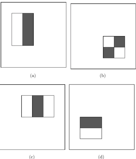
After the integral image is created, features are detected in a rectangular window over a portion of the image. Feature examples are shown in Fig. 2.2. The first two examples are features corresponding to two rectangles, one dark and one light. The second and third represent three and four rectangle features respectively. The features are simple representations of the difference between a dark section of an image and a lighter section.
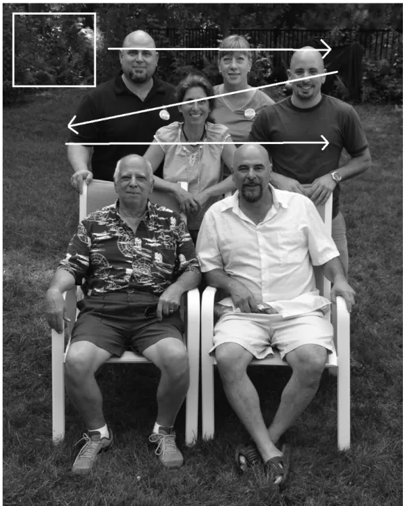
A simple example of what a feature might look like as detected by a classifier in a real image is shown in Fig. 2.3. The feature shown in Fig. 2.3(c)
is used to estimate the difference in pixels’ gray levels between the area covering the eyes and the area below the eyes. A face typically has pixels with lower intensity (darker) along the eye line and pixels with higher intensity (brighter) below. Fig. 2.3(b) shows another possible pattern in which white part of the rectangle template covers the area between the eyes, which consist of brighter
(a) (b)
(c) (d)
Figure 2.2: Four different types of features.
(a) (b) (c)
Figure 2.3: Two different Haar-like features applied to a face.
pixels. The two black parts of the rectangular template cover the eye area, which consist of darker pixels [1].
Figure 2.4: Example of a cascade of classifiers.
2.2.3 Cascade of Classifiers
The detection of features, and thus a face, is accomplished by using a cascade of weak classifiers. A classifier is considered weak when it is
computationally inexpensive and relatively inaccurate, but with an accuracy at least somewhat greater than random. These weak classifiers can then be
cascaded together to form a complete face detection algorithm for a given
window of an image with each additional classifier increasing the accuracy of the algorithm. Sub-windows of the image are rejected at each phase of the cascade, reducing the number of sub-windows that must be processed by the next stage as shown in Fig. 2.4. In this way, the algorithm can have a much shorter runtime than an algorithm with similar accuracy using a single strong classifier.
2.2.4 The Sliding Window
After features have been detected in a given window, the window is moved to a new location in a scanning pattern until all locations in the image have been
Figure 2.5: Example of a scanning window in a test image.
covered. This process is shown in Fig. 2.5. After this, the size of the window is changed and the process starts again in order to detect faces of different sizes.
After the cascade has processed all windows of all sizes, the windows with positive results for faces after passing all classifiers in the cascade have been added to a single list. This list is then processed to combine windows that are
determined to have detected the same face resulting in a final list of detected faces. The end result is a very fast method for face detection [1].
2.3 Related Work
The Viola-Jones face detection algorithm is still one of the more prominent face detection algorithms studied due to its simplicity. Several algorithms have now surpassed its speed and are in use in production
environments, but a large body of research work is still conducted based on the Viola-Jones algorithm. Much of the research effort has been focused on
improving the accuracy of the algorithm since it sacrificed a small amount of accuracy for a large speed gain over algorithms at the time. The authors of [2] attempted to improve the accuracy of the algorithm by passing images through a pre-processing filter before the Viola-Jones algorithm. Their results indicate that for the most part, it is harmful to apply any sort of filter to the image before processing through the Viola-Jones algorithm.
Another attempt at improving the accuracy of the algorithm focuses on pre and post processing using a different method [3]. The authors proposed to first filter out unimportant sections of the image using skin color filtering as well as salient object extraction. Skin color filtering simply selects the area of the image which most likely corresponds to a face by using the color in a particular area. Skin color detection suffers from a large number of false negatives however, so that method is combined with salient object extraction and the two results are combined. Salient object extraction chooses the areas of the image where the
most interesting features are located. The result is then passed through the Viola-Jones algorithm and then once more through the skin color filter. This resulted in a significant decrease in both the false negative rate and the false positive rate bringing both below ten percent.
Although much work has been focused on the accuracy of the Viola-Jones algorithm, there have been many attempts to increase its speed as well using many different approaches. One of these approaches seeks to optimize the algorithm for mobile devices by further simplifying the calculations required [4]. It approaches this problem by assuming that the program will run on weak hardware and reducing the complexity of the algorithm to compensate. The three initial types of optimizations were reducing the size of the image through subsampling before detection, increasing the step size, and increasing the scale factor all in an effort to reduce the number of steps required. In addition, the authors set a minimum face size for detection. The authors were able to achieve a massive increase in throughput implementing all of these optimizations on reduced hardware.
There are also several approaches to increasing the speed of the Viola-Jones algorithm through dedicated hardware. One such approach
synthesized a hardware design using Verilog HDL and ModelSim and were able to achieve 52 frames per second using a 90nm architecture and a 500 MHz clock cycle [5]. Another design using Verilog HDL as well but implemented in a physical FPGA for testing was able to achieve 16 frames per second with an 8 stage classifier [6]. While some of these hardware implementations are very fast,
they are not particularly portable. They only operate on the hardware they were designed for putting them at a disadvantage compared to optimized CPU or GPU algorithms.
There have been several attempts to improve the Viola-Jones algorithm through incorporating GPU processing. One of the most successful attempts was able to get an average speed up of 23x across various resolutions ranging from 340x240 to 1280x1024 [7]. The method that was used was to assign one detection window to one GPU thread. As with many other implementations, this one used several functions present in the OpenCV open source library including the pre-trained frontal-face cascaded classifiers [8]. This approach also implemented the skin color filtering method mentioned earlier. Another similar implementation was able to achieve a maximum speedup of 22x for a 640x480 image using a Nvidia Tesla K40 [9]. This implementation also incorporated diagonal features as well as the simple features originally proposed in the Viola-Jones algorithm to increase accuracy. A third implementation also on GPUs was able to achieve a 12.615x speedup over a high-end Intel Xeon CPU using a Tesla C2050 [10]. Most of these acceleration attempts were done several years ago meaning that the CUDA versions and capabilities of the GPUs are significantly out of date. We believe that there is significant room for improvement with more modern CUDA programming techniques as well as modern GPUs.
While many of these speed increases can sound dramatic, many previous works do not specify details about the configuration of the cascade classifier beyond simple parameters. The number of classifiers in the cascade as well as the
configuration of the cascade can dramatically impact performance. Because of this, it is hard to draw a direct comparison among the performance results of individual works as well as the performance gained by our implementation.
2.4 Summary
In this chapter, we discussed the background of the Viola-Jones algorithm which was designed to increase the speed of face detection while sacrificing very little accuracy. This algorithm was then described in detail, explaining how each step of the algorithm was processed by the CPU. Some related works on
improving the speed and accuracy were also explored to provide a reference point for our improvements to the algorithm.
CHAPTER 3
Parallel Processing Techniques
This chapter provides an overview of parallel processing to provide a framework for understanding the design concepts discussed later in this thesis. A basic overview of parallel processing as a whole will be provided followed by an in-depth explanation of the different types of parallel processing as well as their advantages and disadvantages.
3.1 Basics of Parallel Processing
Many computational problems in today’s world can be split up into many smaller problems that can all be solved simultaneously. Historically, computers have used one processor to solve all of these problems sequentially. With the advent of multicore processors, GPUs, and other types of parallel processors, it is now possible for a computer to execute all of these smaller sub-problems at the same time, increasing the efficiency of the program, thereby decreasing the execution runtime.
3.2 Multithreading
The simplest way to allow a program to take advantage of multiple processing cores is to simply split different tasks up manually and run them on different threads on the CPU. A simple and common example is running
Figure 3.1: Parallel vs. sequential processing.
computationally expensive tasks on a separate thread than the user interface in order to keep the user interface responsive while allowing background processing to continue. This type of multithreading is relatively simple to accomplish and using each thread to its full potential allows for a linear speed increase in processing speed, up to the number of cores in a current generation desktop computer which ranges from two to eight, however high end processors are available with up to 32 physical cores [11][12].
The speedup inherent in parallel processing can be significant and becomes greater with the ability to split a process into many smaller tasks. This is shown in Fig. 3.1 in which a program is split into ”Task 1” and ”Task 2”. In this case, the parallel version in which each task is given its own processing element runs twice as fast as the sequential version in which both tasks run on the same
processing element. This is an ideal scenario, however in other examples, the speedup will not be quite as dramatic. This example assumes both tasks have the same runtime and do not depend on each other in any way. This is not usually the case in most real-world examples since cross thread communication is usually needed, requiring some form of thread synchronization in which one thread must pause and wait for the result from another thread. When this model is expanded to three, four, or more threads, this problem is exacerbated resulting in slowly diminishing returns on the overall processing speed up for adding each thread. Therefore, efficient algorithms for parallelization are needed in order to obtain significant improvements in performance.
3.3 GPGPU
A GPU is a specialized processor used by a computer in order to accelerate graphics output. Graphics processing consists almost completely of highly parallelizable operations. Because of this, GPUs are designed with
hundreds or thousands of simple stream processors which are classified as SIMD. SIMD processors can perform a single function on multiple sets of data at the same time. Since individual cores in a SIMD processor can be much simpler than a core in a standard CPU, more can be included in one processor occupying less space, consuming less power, and at a lower cost. Recently, GPGPU have become more commonly used to solve problems that are highly parallelizable even when the problems are not graphics related. Several programing techniques have been introduced to write code that will execute on GPUs to take advantage
of their highly parallelized nature. The most popular of these languages is CUDA programming, and OpenCL is another example.
3.4 CUDA Programming
Initially, GPU’s were only used for their graphics display capabilities. Around 2003, researchers started to use GPU’s to speed up parallelizable program execution. At the time, it was difficult for someone to use a GPU for general calculations since the program would have to be converted to use either Direct3D or OpenGL, which were the two available graphics APIs at the time. Nvidia and ATI, the two main GPU vendors at the time, saw this potential alternative use for their devices, and Nvidia’s solution was to release CUDA [13]. CUDA is an extension to the C++ programming language provided by Nvidia for programing their graphics processing units [14]. It consists of many basic functions allowing for direct control over the GPU as well as several libraries providing access to preprogramed operations commonly used in massively parallel operations.
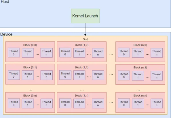
The architecture of an Nvidia GPU as it relates to CUDA programming is shown in Fig. 3.2. A thread is the basic unit of execution as in standard
multithreaded programs, however a thread in CUDA is very different then a thread that would be executed on the CPU. In CUDA, a thread consists of a single data element to be processed since all threads must execute the same instructions due to the limitation of the GPU being a SIMD device, whereas a CPU thread can execute different instructions than other running threads. The threads are created with several different levels of granularity. The first of these
Figure 3.2: CUDA programming structure showing Grids, Blocks, and Threads.
is a warp which consists of 32 threads. A warp is the minimum number of threads that will execute simultaneously. This means that if the programmer only defines enough data for 10 threads, 32 threads worth of GPU power will still be consumed [13].
The next unit of execution is called a block, which can contain anywhere from 64 to 1024 threads, the number of which are dependent on the hardware being used. The number of threads in a block is configurable by the programmer within the hardware limitations. The final unit of execution is called a grid which is made up of multiple blocks. A grid contains all threads which will be executed by a single kernel. Each kernel must be called by the programmer from the host with a set of configuration parameters indicating the block size and the number of blocks [15].
1 g l o b a l v o i d 2 k e r n e l S a m p l e (c o n s t d o u b l e ∗A, d o u b l e ∗C, i n t numElements ) 3 { 4 i n t i = blockDim . x ∗ b l o c k I d x . x + t h r e a d I d x . x ; 5 6 i f ( i < numElements ) 7 { 8 C [ i ] = pow (A[ i ] , 2 ) ; 9 } 10 }
Figure 3.3: Simple kernel example.
The code shown in Fig. 3.3 demonstrates a very simple CUDA kernel example in C++. It looks very similar to a standard function with a few
exceptions. The first notable exception is the use of the "__global__" identifier before the function definition. This indicates that the function is intended to and can only be used to launch a new kernel. Line 4 displays the next significant departure from standard C++. When a kernel is launched, one copy of
vectorAdd is called for each data element provided. The element to be processed is determined by calculating the unique ID of the thread being executed. Line 4 accomplishes this through the use of the blockDim, blockIdx, and threadIdx values. The blockDim variable represents the size of the block and the blockIdx variable represents the location of the block within the grid. Multiplying these two variables together gives the id of the first thread in the block. The threadIdx variable represents the location of the thread within the block, so it is added to the previous product giving the unique thread id. Line 6 checks to ensure that the GPU does no calculations beyond the end of the given arrays. This is
necessary because a GPU can only process threads in multiples of the warp size. If the data does not fit exactly in that number of threads, there will be some threads at the end of the kernel launch that have no data to process. Attempting
1 i n t t h r e a d s P e r B l o c k = 1 2 8 ; 2 i n t b l o c k s P e r G r i d =(numElements + t h r e a d s P e r B l o c k − 1 ) / t h r e a d s P e r B l o c k ; 3 k e r n e l S a m p l e<<<b l o c k s P e r G r i d , t h r e a d s P e r B l o c k>>>(d A , d B , numElements ) ; 4 e r r = c u d a G e t L a s t E r r o r ( ) ;
Figure 3.4: Example of a simple kernel call
to process these threads would result in an exception.
The code shown in Fig. 3.4 demonstrates an example of launching the defined kernel. The number of threads per block and blocks per grid must first be defined by the programmer. The optimal number of threads per block is highly dependent on the code running in the kernel and the hardware being used and will vary from kernel to kernel. The number of blocks per grid is simply the total number of elements divided by the threads per block plus one additional block for any remaining threads that do not fit exactly into increments of the block size. The kernel is then launched similarly to a regular function call except for passing in the block size and grid size as shown in line 3 from Fig. 3.4. The final line gets the status of the kernel after it has finished execution and will contain a success value if the kernel was successful or a description of whatever error was encountered.
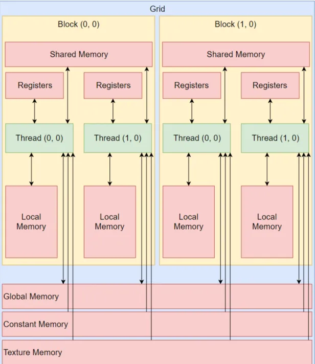
Fig. 3.5shows a schematic representation of the memory organization available to the GPU. Each type of memory has advantages and disadvantages as well as different intended uses. The lowest level memory available to the GPU are registers and local memory. These are only accessible by single threads within a kernel. They are the fastest memory available to the programmer and a limited amount is available per block. This means that if each thread needs a large
Figure 3.5: CUDA programming structure showing layout of memory on a GPU.
quantity of registers, fewer threads can be launched within a single block. Shared memory is shared amongst all of the threads within a block. This memory is useful for calculations in which the results or inputs must be shared amongst a block of threads but not amongst all blocks within a kernel. Registers and shared memory are the fastest memory available to a CUDA programmer and should be
used whenever possible. The main limitation is the relatively small quantity of registers and shared memory available [15].
There are also a number of other types of memory available. Global memory is one of these, which can be accessed by any thread and is also the easiest memory to store and retrieve values from. Global memory is the slowest of the other memory types, but also the largest in size. Global memory access can be somewhat optimized by coalescing memory accesses. This is accomplished by having a thread with index i access the element of an array with index i. This allows the GPU to access all memory for a given warp in one single instruction. If instead thread i needs data from location i+x, the memory locations are not all adjacent and the GPU must break up memory reads into a number of operations, significantly slowing down memory access.
Constant and texture memory both have specific use cases in which each is faster than global memory. Constant memory is best for when all threads within a warp must access the same data. If every thread needs access to a value x in the same instruction, it can be retrieved once and broadcast to all threads in the same operation. Texture memory is optimized for 2D spatial storage and is arguably the most complicated memory type to optimize correctly. Texture memory can coalesce memory accesses for values in a matrix that are close to each other. An example is if the values arr[x][y], arr[x+1][y], arr[x][y+1], and arr[x+1][y+1] are required by four different threads in a warp, texture memory may be able to combine those into a single memory access.
3.5 Comparison of CPU Processing and GPGPU
Standard CPUs and GPUs are very different in both design and intended function. CPUs are MIMD devices and are designed to be able to run a wide range of programs using a few high-speed processor cores. GPUs are SIMD devices that are designed to perform a single calculation on large amounts of data simultaneously. Each individual physical execution unit in the Tesla GPU is only as fast in terms of frequency as each in the Core i7 CPU, however the Tesla has over 700 times as many cores as the Core i7. In addition, the memory
bandwidth of the Tesla is much higher and the overall Floating-Point Operations per Second (FLOPS) is over six times faster. These benefits are however, only enjoyed when executing a highly parallelizable task.
3.6 CUDA C vs Standard C++
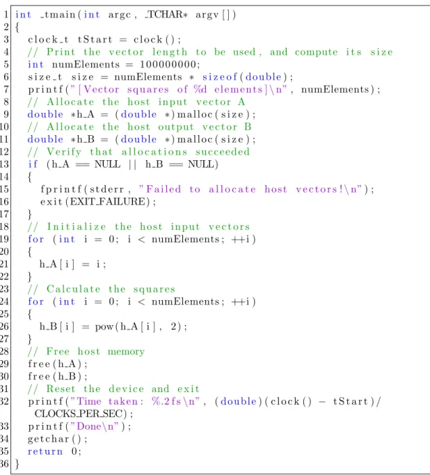
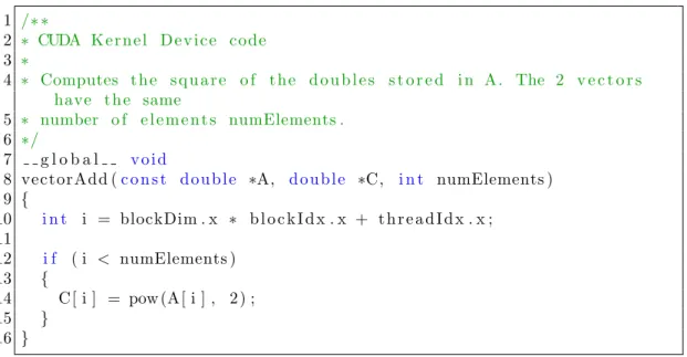
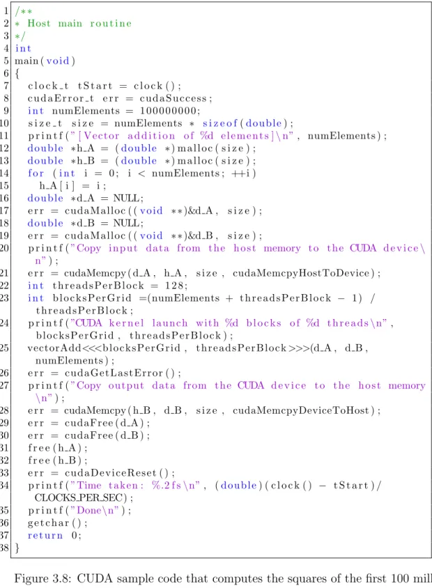
The benefits of GPGPU can be shown through a simple piece of C++ code that computes the squares of the first 100 million integers stored in vectors. The first code segment shown in Fig. 3.6 is the implementation in standard C++. The next code segment shown in Fig. 3.7and Fig. 3.8 performs the exact same calculation as the standard C++ code but utilizes the GPU through CUDA C.
Running on an i7 CPU at 4 GHz, the code took 4.58 seconds to execute. Running on a GTX 670 GPU at 915 MHz, the code took 1.58 seconds to execute. This means that for this particular calculation and implementation, the GPU was able to perform the calculation 3.5x faster than the CPU. The difference between
1 i n t t m a i n (i n t a r g c , TCHAR∗ a r g v [ ] ) 2 {
3 c l o c k t t S t a r t = c l o c k ( ) ;
4 // P r i n t t h e v e c t o r l e n g t h t o be used , and compute i t s s i z e
5 i n t numElements = 1 0 0 0 0 0 0 0 0 ; 6 s i z e t s i z e = numElements ∗ s i z e o f(d o u b l e) ; 7 p r i n t f (” [ V e c t o r s q u a r e s o f %d e l e m e n t s ]\n”, numElements ) ; 8 // A l l o c a t e t h e h o s t i n p u t v e c t o r A 9 d o u b l e ∗h A = (d o u b l e ∗) m a l l o c ( s i z e ) ; 10 // A l l o c a t e t h e h o s t o u t p u t v e c t o r B 11 d o u b l e ∗h B = (d o u b l e ∗) m a l l o c ( s i z e ) ; 12 // V e r i f y t h a t a l l o c a t i o n s s u c c e e d e d 13 i f ( h A == NULL | | h B == NULL) 14 { 15 f p r i n t f ( s t d e r r , ” F a i l e d t o a l l o c a t e h o s t v e c t o r s !\n”) ; 16 e x i t (EXIT FAILURE) ; 17 } 18 // I n i t i a l i z e t h e h o s t i n p u t v e c t o r s 19 f o r (i n t i = 0 ; i < numElements ; ++i ) 20 { 21 h A [ i ] = i ; 22 } 23 // C a l c u l a t e t h e s q u a r e s 24 f o r (i n t i = 0 ; i < numElements ; ++i ) 25 { 26 h B [ i ] = pow ( h A [ i ] , 2 ) ; 27 } 28 // F r e e h o s t memory 29 f r e e ( h A ) ; 30 f r e e ( h B ) ; 31 // R e s e t t h e d e v i c e and e x i t 32 p r i n t f (”Time t a k e n : %.2 f s\n”, (d o u b l e) ( c l o c k ( ) − t S t a r t ) / CLOCKS PER SEC) ;
33 p r i n t f (”Done\n”) ; 34 g e t c h a r ( ) ;
35 r e t u r n 0 ; 36 }
Figure 3.6: C++ sample code that computes the sqares of the first 100 million integers.
a CPU and GPU in terms of processing efficiency varies widely from program to program. Some programs will run slower when compiled on a GPU due to not being parallelizable and the GPU having slower cores. There are also cases when the GPU may execute code over 300x faster than a CPU would be able to. Because of this, determining if it is worthwhile to use GPGPU is dependent on the algorithm being used in the program.
1 /∗ ∗ 2 ∗ CUDA K e r n e l D e v i c e c o d e 3 ∗ 4 ∗ Computes t h e s q u a r e o f t h e d o u b l e s s t o r e d i n A. The 2 v e c t o r s have t h e same 5 ∗ number o f e l e m e n t s numElements . 6 ∗/ 7 g l o b a l v o i d 8 vectorAdd (c o n s t d o u b l e ∗A, d o u b l e ∗C, i n t numElements ) 9 { 10 i n t i = blockDim . x ∗ b l o c k I d x . x + t h r e a d I d x . x ; 11 12 i f ( i < numElements ) 13 { 14 C [ i ] = pow (A[ i ] , 2 ) ; 15 } 16 }
Figure 3.7: CUDA sample kernel to compute the square of one array and save it into another array.
1 /∗ ∗ 2 ∗ Host main r o u t i n e 3 ∗/ 4 i n t 5 main (v o i d) 6 { 7 c l o c k t t S t a r t = c l o c k ( ) ; 8 c u d a E r r o r t e r r = c u d a S u c c e s s ; 9 i n t numElements = 1 0 0 0 0 0 0 0 0 ; 10 s i z e t s i z e = numElements ∗ s i z e o f(d o u b l e) ; 11 p r i n t f (” [ V e c t o r a d d i t i o n o f %d e l e m e n t s ]\n”, numElements ) ; 12 d o u b l e ∗h A = (d o u b l e ∗) m a l l o c ( s i z e ) ; 13 d o u b l e ∗h B = (d o u b l e ∗) m a l l o c ( s i z e ) ; 14 f o r (i n t i = 0 ; i < numElements ; ++i ) 15 h A [ i ] = i ; 16 d o u b l e ∗d A = NULL ; 17 e r r = c u d a M a l l o c ( (v o i d ∗ ∗)&d A , s i z e ) ; 18 d o u b l e ∗d B = NULL ; 19 e r r = c u d a M a l l o c ( (v o i d ∗ ∗)&d B , s i z e ) ;
20 p r i n t f (”Copy i n p u t d a t a from t h e h o s t memory t o t h e CUDA d e v i c e\
n”) ; 21 e r r = cudaMemcpy ( d A , h A , s i z e , cudaMemcpyHostToDevice ) ; 22 i n t t h r e a d s P e r B l o c k = 1 2 8 ; 23 i n t b l o c k s P e r G r i d =(numElements + t h r e a d s P e r B l o c k − 1 ) / t h r e a d s P e r B l o c k ; 24 p r i n t f (”CUDA k e r n e l l a u n c h w i t h %d b l o c k s o f %d t h r e a d s\n”, b l o c k s P e r G r i d , t h r e a d s P e r B l o c k ) ; 25 vectorAdd<<<b l o c k s P e r G r i d , t h r e a d s P e r B l o c k>>>(d A , d B , numElements ) ; 26 e r r = c u d a G e t L a s t E r r o r ( ) ;
27 p r i n t f (”Copy o u t p u t d a t a from t h e CUDA d e v i c e t o t h e h o s t memory
\n”) ; 28 e r r = cudaMemcpy ( h B , d B , s i z e , cudaMemcpyDeviceToHost ) ; 29 e r r = c u d a F r e e ( d A ) ; 30 e r r = c u d a F r e e ( d B ) ; 31 f r e e ( h A ) ; 32 f r e e ( h B ) ; 33 e r r = c u d a D e v i c e R e s e t ( ) ; 34 p r i n t f (”Time t a k e n : %.2 f s\n”, (d o u b l e) ( c l o c k ( ) − t S t a r t ) / CLOCKS PER SEC) ;
35 p r i n t f (”Done\n”) ; 36 g e t c h a r ( ) ;
37 r e t u r n 0 ; 38 }
Figure 3.8: CUDA sample code that computes the squares of the first 100 million integers.
CHAPTER 4
Parallelization Approaches of the Viola-Jones Face Detection Algorithm
This chapter provides a description of the original Viola-Jones algorithm implementation. It also provides design concepts for several different new versions of the Viola-Jones face detection algorithm. These approaches include two different multithreaded versions as well as a CUDA version. These concepts provide the basis for the implementations in Chapter 5.
4.1 Original Design
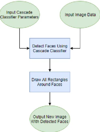
The original design for the Viola-Jones face detection algorithm uses a Haar cascade classifier object detection filter to process a PMG format image. The program follows the structure shown in the diagram from Fig. 4.1. Pseudocode for the program structure is shown in Fig. 4.2The program first loads cascade classifier parameters out of a text file. These parameters have been determined programmatically through training prior to use of the algorithm. The image is also loaded into the program from the same location. The input image is then processed through the algorithm with the result being rectangle objects consisting of four coordinate locations on the image representing a detected face. These rectangles are then drawn onto the image and the result is saved into a new PMG image file for viewing.
Figure 4.1: Basic structure of the face detection program. 1 main ( ) 2 { 3 s t a r t t i m e r ; 4 l o a d image from d i s k ; 5 l o a d c a s c a d e c l a s s i f i e r p a r a m e t e r s from d i s k ; 6 r e s u l t s = d e t e c t O b j e c t s ( image , c l a s s i f i e r ) ; 7 f o r e a c h ( r e s u l t i n r e s u l t s ) 8 { 9 draw r e c t a n g l e around f a c e ; 10 } 11 s a v e m o d i f i e d image t o d i s k ; 12 f r e e c l a s s i f i e r ; 13 f r e e image ; 14 s t o p t i m e r ; 15 p r i n t t i m e t a k e n ; 16 }
Figure 4.2: Main program structure.
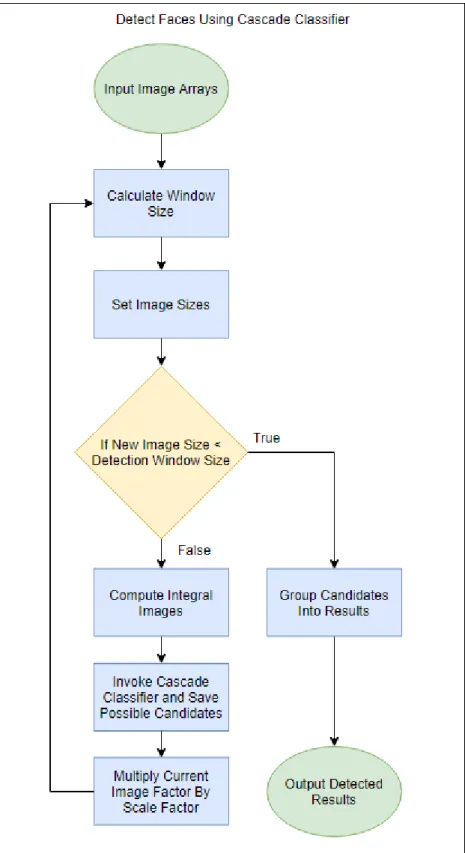
The detect objects process runs as shown in the flowchart from Fig. 4.3. Pseudocode for the detect objects process is shown in Fig. 4.4. The chart shows the loop that the detection algorithm runs in for the majority of the program’s
Figure 4.3: Structure of the face detection function. This diagram represents the process in the block labeled “Detect Faces Using Cascade Classifier” in Fig. 4.1.
1 d e t e c t O b j e c t s ( image , c l a s s i f i e r ) 2 { 3 c r e a t e image a r r a y s ; 4 f o r( f a c t o r = 1 ; f a c t o r ∗= s c a l e f a c t o r ) 5 { 6 c a l c u l a t e window s i z e ; 7 s e t image s i z e s ; 8 compute i n t e g r a l i m a g e s ; 9 s e t i m a g e s f o r c l a s s i f i e r ; 10 c l a s s i f i e r I n v o k e r ( ) ; 11 } 12 group c a n d i d a t e s i n t o r e s u l t s ; 13 f r e e a l l i m a g e s ; 14 r e t u r n r e s u l t s ; 15 }
Figure 4.4: Initial object detection structure.
duration. The number of iterations is dependent on the scale factor which can be decreased to improve accuracy at the expense of runtime or vice versa.
Depending on the scale factor, the outer loop from Fig. 4.3will run
approximately 10 to 20 times. This makes it a good possibility to implement CPU multithreading since the number of threads to be run for a performance increase is limited by the number of cores in a processor.
The classifier runs as shown in Fig. 4.5. Pseudocode for the classifier is shown in Fig. 4.6. This diagram shows the internal workings of the classifier itself. Using the input values of the image arrays and window size values, the classifier starts at location (0,0). At each location, the classifier is evaluated and any results that are obtained are saved. The window is then moved to a new location determined by the stepsize and the process is repeated. As can be seen, the base process “Evaluate Classifier at Location” runs potentially thousands of times over the course of algorithm execution considering the number of large nested loops. This makes it potentially a good place to optimize using CUDA if
the necessary data can be provided to all threads simultaneously.
The main optimization opportunity here involves the running of the face detection function and classifier. At what level to optimize is highly dependent on the method of optimization chosen. Multithreaded programs run on a small number of powerful threads, meaning that the program only needs to be broken up into a few pieces to fully optimize the code for a multi-core CPU. CUDA however runs on graphics cards that have thousands of small processor cores resulting in the need for a more fine-grained division of work.
4.2 Design of Multithreaded Face Detection Algorithm
When considering the design for the multithreaded version, the first proposal involved multithreading the outer loop. This seemed to be a good design decision since thread creation is an expensive process. This type of multithreading would ideally create enough threads to result in a speedup but not so many that the cost of thread generation outweighed the performance gain. The corresponding version of the block diagram is shown in Fig. 4.7. The
pseudocode is provided in Fig. 4.8. The functionality and processes shown in this diagram are meant to replace the functionality in Fig. 4.3.
After the initial consideration, this approach was abandoned due to the great variation in the time taken to run each iteration of the scale factor loop. The first created threads ran for exponentially longer time than the final threads created as shown in Fig. 4.9, and while this approach resulted in some speedup, it was far from the potential optimum performance. Ideally, all threads would
run at full usage for the entire runtime of the program and that was not the case with this solution.
The second considered solution involved creating a set of worker threads for each iteration and assigning them jobs to multithread the detecting of
potential candidates. This approach, while a bit more complicated to implement, turned out to be vastly superior in terms of performance. This optimization is intended to replace the functionality in Fig. 4.3.
As shown in Fig. 4.10, each factor has its work split up into equal size chunks, the number of chunks being equal to the number of threads available in the system. This will allow the program to take full advantage of every core in the system while also ensuring that every thread has as close to an equal amount of work as possible. This design is slightly more complicated than the one
displayed in Fig. 4.7, but still fairly simple to implement resulting in substantial performance gains for the extra effort involved. Pseudocode for this solution is provided in Fig. 4.11.
4.3 Design of CUDA Face Detection Algorithm
Converting an existing algorithm to work on a GPU is more complicated than simply multithreading it on a CPU. In order to effectively utilize a GPU, the program must perform the same calculation hundreds or, ideally, thousands of times on different data. Because of this, the logical place to implement a CUDA kernel in this project is in a similar place as the final solution for the multithreaded version.
As shown in Fig. 4.12, the overall design of the CUDA version does not have very many additional steps. Instead of using the number of threads as in the multithreaded version, a blocksize is set by the programmer. This
implementation parameter will be tested with several values to find the optimal setting for this particular parallelization approach. The number of blocks is then simply the number of steps divided by the blocksize. In this proposal, one kernel launch will take place for each factor in the outer loop. This optimization is intended to replace the cascade classifier invoker shown in Fig. 4.5. The pseudocode for this solution is shown in Fig. 4.13.
4.4 Summary
In this chapter, we provided several design concepts for future
implementation in Chapter 5. These included a multithreaded concept and a CUDA concept. The original design was also discussed to provide a framework for our improvements.
Figure 4.5: Structure of the classifier function. This diagram represents the process in the block labled “Invoke Cascade Classifier” in Fig. 4.3.
1 c l a s s i f i e r I n v o k e r ( ) 2 { 3 g e t window s i z e ; 4 f o r( x = 0 ; x < x2 ; x += s t e p ) 5 { 6 f o r( y = y1 ; y < y2 ; y += s t e p ) 7 { 8 s e t window l o c a t i o n ; 9 run c l a s s i f i e r ; 10 i f r e s u l t i s p r e s e n t , add r e s u l t t o c a n d i d a t e s l i s t ; 11 } 12 } 13 }
Figure 4.7: First proposal for a multithreaded optimization of the object detection function.
1 d e t e c t O b j e c t s ( image , c l a s s i f i e r ) 2 { 3 c r e a t e image a r r a y s ; 4 f o r( f a c t o r = 1 ; f a c t o r ∗= s c a l e f a c t o r ) 5 { 6 s t a r t t h r e a d => 7 { 8 c a l c u l a t e window s i z e ; 9 s e t image s i z e s ; 10 b u i l d image pyramid ; 11 compute i n t e g r a l i m a g e s ; 12 s e t i m a g e s f o r c l a s s i f i e r ; 13 c l a s s i f i e r I n v o k e r ( ) ; 14 } 15 } 16 w a i t f o r a l l t h r e a d s t o c o m p l e t e ; 17 group c a n d i d a t e s i n t o r e s u l t s ; 18 f r e e a l l i m a g e s ; 19 r e t u r n r e s u l t s ; 20 }
Figure 4.8: First proposal for a multithreaded optimization of the object detection function psudocode.
Figure 4.9: Number of steps performed by each thread. The variation is due to each iteration having a different scale factor.
Figure 4.10: Seccond proposal for a multithreaded optimization of the object de-tection function.
1 d e t e c t O b j e c t s ( image , c l a s s i f i e r ) 2 { 3 c r e a t e image a r r a y s ; 4 f o r( f a c t o r = 1 ; f a c t o r ∗= s c a l e f a c t o r ) 5 { 6 c a l c u l a t e window s i z e ; 7 s e t image s i z e s ; 8 b u i l d image pyramid ; 9 compute i n t e g r a l i m a g e s ; 10 s e t i m a g e s f o r c l a s s i f i e r ; 11 c a l c u l a t e t o t a l number o f s t e p s i n i n v o k e r ; 12 g e t t o t a l number o f hardware t h r e a d s ; 13 c a l c s P e r T h r e a d = t o t a l s t e p s / number o f t h r e a d s ; 14 f o r( i = 0 ; i < numThreads ; i ++) 15 { 16 t h r e a d S t a r t L o c a t i o n = i ∗ c a l c s P e r T h r e a d ; 17 t h r e a d S t o p L o c a t i o n = ( i + 1 ) ∗ c a l c s P e r T h r e a d ; 18 c r e a t e and s t a r t t h r e a d ( doThreadWork , c l a s s i f i e r , t h r e a d S t a r t L o c a t i o n , t h r e a d S t o p L o c a t i o n ) ; 19 } 20 w a i t f o r a l l t h r e a d s t o f i n i s h ; 21 } 22 group c a n d i d a t e s i n t o r e s u l t s ; 23 f r e e a l l i m a g e s ; 24 r e t u r n r e s u l t s ; 25 }
Figure 4.11: Second proposal for a multithreaded optimization of the object de-tection function psudocode.
Figure 4.12: Proposal for a CUDA replacement for the “invoke cascade classifier” function.
1 c l a s s i f i e r I n v o k e r ( ) 2 { 3 g e t window s i z e ; 4 c a l c u l a t e t o t a l number o f s t e p s i n i n v o k e r ; 5 s e t t h e b l o c k s i z e ; 6 numblocks = t o t a l s t e p s / b l o c k s i z e ;
7 s t a r t k e r n e l w i t h b l o c k s i z e and number o f b l o c k s t o run c l a s s i f i e r ;
8 w a i t f o r k e r n e l t o f i n i s h ; 9 }
CHAPTER 5
Implementation Details
This chapter will describe in detail how each implementation was created. These implementations include a multithreaded version with the capability to run on any x86 architecture processor as well as a CUDA version able to run on any Nvidia CUDA capable GPU. This chapter will only cover changes made to the original code and not any aspects that were left the same as the original.
5.1 Implementation of Multithreaded Face Detection Algorithm
The implementation of the parallelization approach described in Chapter
4 is fairly simple in comparison with the CUDA version. The section of the original classifier invoker design is shown in Fig. 5.1, and the new design is shown in Fig. 5.2and Fig. 5.3
As can be seen in Fig. 5.2, the new implementation creates a vector of threads and bases the number of threads to be used on the hardware concurrency available in the system. It then creates threads one by one using the
doThreadWork method and passing the correct work data values using
i*calcsPerStep and (i + 1)*calcsPerStep. Lines 9-10 join each thread to the main thread preventing work on the main thread from continuing until all spawned threads have finished.
1 i n t s t e p s = 0 ; 2 f o r( x = 0 ; x < x2 ; x += s t e p ) 3 { 4 f o r( y = y1 ; y < y2 ; y += s t e p ) 5 { 6 p . x = x ; 7 p . y = y ; 8 r e s u l t = r u n C a s c a d e C l a s s i f i e r ( c a s c a d e , p , 0 ) ; 9 s t e p s ++; 10 i f( r e s u l t > 0 ) 11 {
12 MyRect r = {myRound ( x∗f a c t o r ) , myRound ( y∗f a c t o r ) , w i n S i z e . width , w i n S i z e . h e i g h t};
13 vec−>p u s h b a c k ( r ) ;
14 }
15 }
16 }
Figure 5.1: Original implementation of classifier invoker.
1 i n t s t e p s = x2 ∗ ( y2 − y1 ) ; 2 i n t numthreads = s t d : : t h r e a d : : h a r d w a r e c o n c u r r e n c y ( ) ; 3 i n t c a l c s P e r S t e p = s t e p s / numthreads ; 4 s t d : : v e c t o r<s t d : : t h r e a d> t h r e a d s ; 5 f o r (i n t i = 0 ; i ∗ c a l c s P e r S t e p < s t e p s ; i ++) 6 { 7 t h r e a d s . p u s h b a c k ( s t d : : t h r e a d ( doThreadWork , x2 , c a s c a d e , f a c t o r , i∗c a l c s P e r S t e p , ( i + 1 )∗c a l c s P e r S t e p , v e c , w i n S i z e , s t e p s ) ) ; 8 } 9 f o r (i n t i = 0 ; i ∗ c a l c s P e r S t e p < s t e p s ; i ++) 10 t h r e a d s [ i ] . j o i n ( ) ;
Figure 5.2: New implementation of classifier invoker.
of the work based on a lowerBound and an upperBound. Because the number of steps may not always be a multiple of the number of threads created, it must check if it has passed the total number of steps and exit the method if it has. An area of note is lines 14-16. Because this code is being executed on multiple
threads simultaneously, it is possible to call _vec.push_back() multiple times at the same instant. In order to avoid this, a mutex must be used to only allow one thread to add a value to the vector at one time instance. Once a thread obtains a lock on the mutex, all other threads will suspend execution on the lock command
1 v o i d doThreadWork (i n t maxX , myCascade∗ c a s c a d e , f l o a t f a c t o r , i n t lowerBound , i n t upperBound , s t d : : v e c t o r<MyRect>& v e c , MySize w i n S i z e , i n t t o t a l S t e p s ) 2 { 3 // i n i t i a l i z a t i o n work 4 f o r(i n t i = lowerBound ; i < upperBound ; i ++) 5 { 6 i f ( i > t o t a l S t e p s ) 7 r e t u r n; 8 p . x = i % maxX ; 9 p . y = ( i − p . x ) / maxX ; 10 r e s u l t = r u n C a s c a d e C l a s s i f i e r ( c a s c a d e , p , 0 ) ; 11 i f ( r e s u l t > 0 ) 12 {
13 MyRect r = { myRound ( p . x∗f a c t o r ) , myRound ( p . y∗f a c t o r ) , w i n S i z e . width , w i n S i z e . h e i g h t }; 14 p u s h b a c k m u t e x . l o c k ( ) ; 15 v e c . p u s h b a c k ( r ) ; 16 p u s h b a c k m u t e x . u n l o c k ( ) ; 17 } 18 } 19 }
Figure 5.3: Thread work method.
until the original thread has released its lock. This prevents cross-thread exceptions in this implementation.
Another item of note is the simplicity of implementing this code. The percentage of code required to be modified from the overall program was fairly insignificant and the modification process was very straightforward. This
implementation resulted in a significant speedup as will be discussed in Chapter
1 i n t c [N ] ; 2 // f i l l a r r a y h e r e 3 i n t ∗d e v c ; 4 c u d a M a l l o c ( (v o i d∗ ∗) &d e v c , N ∗ s i z e o f(i n t) ) ; 5 cudaMemcpy ( d e v c , c , N ∗ s i z e o f(i n t) , cudaMemcpyHostToDevice ) ; 6 // do s o m e t h i n g on d e v i c e h e r e 7 cudaMemcpy ( c , d e v c , N ∗ s i z e o f(i n t) , cudaMemcpyDeviceToHost ) ; 8 c u d a F r e e ( d e v c ) ;
Figure 5.4: Copy data using cudaMemcpy.
5.2 Implementation of CUDA Face Detection Algorithm
5.2.1 Initial Considerations and Preparatory Work
The CUDA implementation, despite being arguably simpler in design than the multithreaded version turned out to be significantly more complex. There were many more considerations involved when processing code on a GPU. The first of these considerations and arguably the most important is the fact that data that is stored in system RAM is not directly accessible by the GPU. When a kernel has to be launched, first it should be confirmed that all data has been transferred into some of the GPU memory types.
As shown in Fig. 5.4, copying data back and forth from the system RAM to the GPU global memory is a relatively complex process. Similar to how
memory works in system RAM, space must first be allocated using cudaMalloc to which the data will be copied using cudaMemcpy. This process must be
performed for every piece of data needed on the GPU [16]. Luckily, starting with CUDA version 6, there is a new method of copying data using unified memory as shown in Fig. 5.5.
1 i n t ∗d a t a 2 cudaMallocManaged(&data , N) ; 3 // f i l l a r r a y h e r e 4 // do s o m e t h i n g on d e v i c e h e r e 5 // u s e d a t a on h o s t h e r e 6 c u d a F r e e ( d a t a ) ;
Figure 5.5: Copy data using unified memory.
only once, which allocates memory on both the host and the device. The data is then copied automatically back and forth from host to device as necessary. Because of this simplicity in comparison to the original method of memory management, the method shown in Fig. 5.5 was chosen for this program.
In addition, a new feature implemented in CUDA 8 and only available on Pascal architecture GPUs is the Page Migration Engine [17]. Previously,
allocated unified memory would all be moved as one large transaction before a kernel was launched. With the Page Migration Engine in Pascal, page faulting from CPU to GPU and back has been implemented allowing the GPU to request individual pages as necessary to be transferred instead of transferring all the data at once. This allows for more computation-memory transfer overlap when
running multiple kernels, increasing performance. For example. Kernel A can be transferring data due to a page fault while Kernel B is using the GPUs
processing power.
A final addition is the ability to request an asynchronous prefetch of data well before kernel launch. If it is known that Kernel A is going to need an entire dataset, it could potentially hurt performance to allow the GPU to page fault on every data access and have to wait for the data to be transferred hundreds of individual times. In this case, the memory can be prefetched to the GPU any
1 #d e f i n e gpuErrchk ( ans ) { g p u A s s e r t ( ( ans ) , F I L E , L I N E ) ; } 2 i n l i n e v o i d g p u A s s e r t ( c u d a E r r o r t code , c o n s t c h a r ∗f i l e , i n t l i n e , b o o l a b o r t = t r u e) 3 { 4 i f ( c o d e != c u d a S u c c e s s ) 5 { 6 f p r i n t f ( s t d e r r , ” GPUassert : %s %s %d\n”, c u d a G e t E r r o r S t r i n g ( c o d e ) , f i l e , l i n e ) ; 7 i f ( a b o r t ) e x i t ( c o d e ) ; 8 } 9 } 10 11 c l a s s Managed 12 { 13 p u b l i c: 14 v o i d ∗o p e r a t o r new( s i z e t l e n ) 15 { 16 v o i d ∗p t r ; 17 gpuErrchk ( cudaMallocManaged(& p t r , l e n ) ) ; 18 c u d a D e v i c e S y n c h r o n i z e ( ) ; 19 r e t u r n p t r ; 20 } 21 v o i d ∗o p e r a t o r new[ ] ( s i z e t l e n ) 22 { 23 v o i d ∗p t r ; 24 cudaMallocManaged(& p t r , l e n ) ; 25 c u d a D e v i c e S y n c h r o n i z e ( ) ; 26 r e t u r n p t r ; 27 } 28 v o i d o p e r a t o r d e l e t e(v o i d ∗p t r ) 29 { 30 c u d a D e v i c e S y n c h r o n i z e ( ) ; 31 c u d a F r e e ( p t r ) ; 32 } 33 };
Figure 5.6: CUDA managed class.
time before the kernel is launched. This call is asynchronous meaning that CPU execution continues after starting the transaction allowing CPU execution to overlap with the memory transfer. After much testing, it was determined that in our version of the algorithm, it provided the best performance to not prefetch any data and allow the GPU to handle page faults and migration.
In order to facilitate ease of use for objects on both the host and CUDA device, a Managed class was created as shown in Fig. 5.6. All non-primitive
1 #d e f i n e NODES 3000 2 #d e f i n e STAGES 100 3 c o n s t a n t s h o r t d a l p h a 1 a r r a y [NODES ] ; 4 c o n s t a n t s h o r t d a l p h a 2 a r r a y [NODES ] ; 5 c o n s t a n t s h o r t d s t a g e s t h r e s h a r r a y [ STAGES ] ; 6 c o n s t a n t s h o r t d w e i g h t s a r r a y [NODES∗3 ] ; 7 c o n s t a n t s h o r t d s t a g e s a r r a y [ STAGES ] ; 8 c o n s t a n t s h o r t d t r e e t h r e s h a r r a y [NODES ] ;
Figure 5.7: CUDA constant variables defined.
types that need to be accessed at some point on the GPU and CPU inherit from this Managed class in the program. The first nine lines are present to allow for GPU error checking on every GPU command. The managed class overrides the new operators for both single objects and arrays of objects. This forces objects created from types that inherit from the Managed class to be allocated using CUDA unified memory by just using the standard new method. The delete operator is also overridden to facilitate freeing of unified memory.
5.2.2 Object Creation and Allocation Decisions
Despite the changes made to basic object allocation, there are still a few decisions that must be made before proceeding with kernel design. Primitive types and arrays still must be allocated manually. In addition to this, it must be considered how the memory will be accessed. If every kernel will use the same values, it is best to assign the data to constant device memory, but if the values must change, global memory must be used. How the variables are handled differs depending on the allocation choice made for each one.
Several arrays are used by every kernel over the course of program execution and are only read from by the kernels, never written to. These arrays
1 gpuErrchk ( cudaMemcpyToSymbol ( d t r e e t h r e s h a r r a y , t r e e t h r e s h a r r a y , s i z e o f(i n t)∗t o t a l n o d e s ) ) ; 2 gpuErrchk ( cudaMemcpyToSymbol ( d a l p h a 1 a r r a y , a l p h a 1 a r r a y , s i z e o f( i n t)∗t o t a l n o d e s ) ) ; 3 gpuErrchk ( cudaMemcpyToSymbol ( d a l p h a 2 a r r a y , a l p h a 2 a r r a y , s i z e o f( i n t)∗t o t a l n o d e s ) ) ; 4 gpuErrchk ( cudaMemcpyToSymbol ( d w e i g h t s a r r a y , w e i g h t s a r r a y , s i z e o f (i n t)∗t o t a l n o d e s∗3 ) ) ; 5 gpuErrchk ( cudaMemcpyToSymbol ( d s t a g e s t h r e s h a r r a y , s t a g e s t h r e s h a r r a y , s i z e o f(i n t)∗s t a g e s ) ) ; 6 gpuErrchk ( cudaMemcpyToSymbol ( d s t a g e s a r r a y , s t a g e s a r r a y , s i z e o f( i n t)∗s t a g e s ) ) ;
Figure 5.8: CUDA constant variables copied to.
1 gpuErrchk ( cudaMallocManaged(& s c a l e d r e c t a n g l e s a r r a y , s i z e o f(i n t∗)
∗t o t a l n o d e s∗( 1 2 + 0 ) ) ) ;
Figure 5.9: CUDA objects allocated in global memory.
are best assigned to constant memory as shown in Fig. 5.7. These arrays were originaly int arrays in the initial version of the program. They were changed to shorts after confirming that it would not harm accuracy to allow all of the constant readonly data to fit in the constant memory available on the GPU. These variables are copied to by using the cudaMemcpyToSymbol function as shown in Fig. 5.8. The scaled_rectangles_array is used many times over the course of execution and is therefore placed in global memory as shown in Fig.
5.9.
5.2.3 Kernel Implementation
The CUDA kernel functions are significantly different from the
multithreaded implementation. Because there is no way to provide thread safe access to a vector in CUDA for depositing results, a different approach must be
1 i n t s t e p s = x2 ∗ ( y2 − y1 ) ; 2 i n t b l o c k s i z e = 1 2 8 ;
3 i n t numblocks = (i n t) s t e p s / b l o c k s i z e ; 4 i f ( numblocks < 1 )
5 numblocks = 1 ;
6 MyRect∗ r e c t L i s t = new MyRect [ numblocks ∗ b l o c k s i z e ] ; 7 gpuErrchk ( c u d a D e v i c e S y n c h r o n i z e ( ) ) ; 8 S h i f t F i l t e r C u d a << <numblocks , b l o c k s i z e >> >(x2 , ∗c a s c a d e , f a c t o r , w i n S i z e , r e c t L i s t , s c a l e d r e c t a n g l e s a r r a y ) ; 9 gpuErrchk ( c u d a P e e k A t L a s t E r r o r ( ) ) ; 10 gpuErrchk ( c u d a D e v i c e S y n c h r o n i z e ( ) ) ; 11 f o r (i n t i = 0 ; i < numblocks ∗ b l o c k s i z e ; i ++) 12 { 13 i f ( r e c t L i s t [ i ] . h e i g h t != 0 ) 14 vec−>p u s h b a c k ( r e c t L i s t [ i ] ) ; 15 }
Figure 5.10: CUDA kernel preperation and call.
taken. In this call, an array is passed in containing an empty space for every possible result. This array is then checked after the kernel has run in the last five lines in Fig. 5.10 and all valid results are pulled out and added to the vector. The final chosen blocksize was 128 threads in a block. This was used to calculate the total number of blocks needed. The kernel was then launched with the call to cudaPeekAtLastError in order to detect kernel errors.
The kernel itself, displayed in Fig. 5.11, is very simple. It obtains the proper index for thread calculation from the blockIdx, blockDim, and threadIdx as described earlier in Chapter 3. If a result is present after running the classifier on a particular index, the value is saved to the results array for later retrieval.
5.3 Summary
In this chapter, we covered the implementations for each of the design concepts discussed in Chapter4. This includes a multithreaded version that can
1 g l o b a l v o i d
2 S h i f t F i l t e r C u d a (i n t maxX , myCascade &c a s c a d e , f l o a t f a c t o r , MySize w i n S i z e , MyRect∗ r e c t s , i n t∗∗ s c a l e d r e c t a n g l e s a r r a y ) 3 { 4 i n t i = b l o c k I d x . x ∗ blockDim . x + t h r e a d I d x . x ; 5 MyPoint p ; 6 p . x = i % maxX ; 7 p . y = ( i − p . x ) / maxX ; 8 i n t r e s u l t = r u n C a s c a d e C l a s s i f i e r (& c a s c a d e , p , 0 , s c a l e d r e c t a n g l e s a r r a y ) ; 9 i f ( r e s u l t > 0 ) 10 { 11 r e c t s [ i ] . x = myRound ( p . x ∗ f a c t o r ) ; 12 r e c t s [ i ] . y = myRound ( p . y ∗ f a c t o r ) ; 13 r e c t s [ i ] . width = w i n S i z e . width ; 14 r e c t s [ i ] . h e i g h t = w i n S i z e . h e i g h t ; 15 } 16 }
Figure 5.11: CUDA kernel implementation.
run with as many cores as available in the hardware it is run on, as well as a CUDA version capable of running on any CUDA capable GPU. The performance of these implementations as well as the original will be explored in Chapter 6.