Seung Wook Leea)
CT/Micro-CT Lab., Department of Radiology, University of Iowa, Iowa City, Iowa 52242 and Department of Nuclear and Quantum Engineering, Korea Advanced Institute of Science and Technology, Daejeon, 305-701, South Korea
Ge Wanga)
CT/Micro-CT Lab., Department of Radiology, University of Iowa, Iowa City, Iowa 52242
共Received 30 May 2002; accepted for publication 23 January 2003; published 26 March 2003兲 Modern CT and micro-CT scanners are rapidly moving from fan-beam toward cone-beam geom-etry. Half-scan CT algorithms are advantageous in terms of temporal resolution, and widely used in fan-beam and cone-beam geometry. While existing half-scan algorithms for cone-beam CT are in the Feldkamp framework, in this paper we compensate missing data explicitly in the Grangeat framework, and formulate a half-scan algorithm in the circular scanning case. The half-scan spans 180° plus two cone angles that guarantee sufficient data for reconstruction of the midplane defined by the source trajectory. The smooth half-scan weighting functions are designed for the suppression of data inconsistency. Numerical simulation results are reported for verification of our formulas and programs. This Grangeat-type half-scan algorithm produces excellent image quality, without off-mid-plane artifacts associated with Feldkamp-type scan algorithms. The Grangeat-type half-scan algorithm seems promising for quantitative and dynamic biomedical applications of CT and micro-CT. © 2003 American Association of Physicists in Medicine. 关DOI: 10.1118/1.1562941兴 Key words: Computed tomography 共CT兲, cone-beam geometry, half-scan, Grangeat-type reconstruction
I. INTRODUCTION
Modern CT and micro-CT scanners are rapidly moving from fan-beam toward cone-beam geometry.1,2 The half-scan mode is valuable, because it shortens the data acquisition time and improves temporal resolution. Hence, half-scan CT algorithms are widely used in fan-beam and cone-beam geometry.2–5 While existing half-scan algorithms for cone-beam CT are in the Feldkamp framework,2,4 – 6we propose a Grangeat-type half-scan algorithm in the circular scanning case. Our motivation is to perform appropriate data filling using the Grangeat approach,7 and suppress the off-mid-plane artifacts associated with the Feldkamp-type algorithms.8 Interestingly, it came to our attention that Noo and Heuscher just published a half-scan cone-beam recon-struction paper in a SPIE conference.9 Their work is also based on the Grangeat algorithm but it is in the filtered back-projection framework,10while ours is in the rebinning frame-work. The differences between the two Grangeat-type half-scan algorithms will be highlighted in Sec. IV.
This paper is organized as follows. In the next section, we modify Grangeat’s formula for circular half-scan geometry, by combining redundant data to improve contrast resolution while optimizing temporal resolution. The redundant data are weighted with smooth functions to suppress data inconsis-tency. In Sec. III, we describe our software simulator and experimental design, and include images reconstructed from simulated projections of a spherical phantom and the Shepp– Logan phantom. In the last section, we discuss relevant is-sues, and conclude the paper.
II. MATERIALS AND METHODS A. Grangeat framework
As shown in Fig. 1, the radon transform of a three-dimensional 共3-D兲function f (xជ) is defined by
R f共nជ兲⫽
冕
⫺⬁ ⬁冕
⫺⬁ ⬁冕
⫺⬁ ⬁ f共xជ兲␦共xជ"nជ⫺兲dxជ, 共1兲where nជ is the unit vector that passes through the character-istic point C described by spherical coordinates 共,, 兲, xជ Cartesian coordinates 共x, y, z兲. Equation 共1兲 means that the radon value at C is the integral of the object function f (xជ) on the plane through C and normal to the vector nជ. It is well known that the 3-D function f (xជ) can be reconstructed from R f (nជ) provided that R f (nជ) is available for all planes through a neighborhood of point xជ. The inversion formula of the 3-D radon transform is given by
f共xជ兲⫽ ⫺1 82
冕
⫽⫺/2 /2冕
⫽0 2 2 2R f关共xជ"nជ兲nជ兴兩sin兩dd. 共2兲 For beam CT, it is instrumental to connect cone-beam data to 3-D radon data. Smith, Tuy, and Grangeat in-dependently established such connections.7,11,12 Grangeat’s formulation is geometrically attractive and becomes popular. Mathematically, as shown in Fig. 2, the link can be expressed as follows: R f共nជ兲⫽R
⬘
f共nជ兲 ⫽cos12 s冕
⫺⬁ ⬁ SO SA X f关s共nជ兲,t,共nជ兲兴dt ⫽ 1 cos2 s冕
⫺⬁ ⬁ Xwf关s共nជ兲,t,共nជ兲兴dt, 共3兲 where X f关s(nជ),t,(nជ)兴is the detector value the distance s away from the detector center O along the line t perpen-dicular to OCD on the detector plane D located at theangle from the y axis, SO denotes the distance between the source and the origin, SA the distance between the source and an arbitrary point A along t,the angle between the line SO and SC, and Xwf关s(nជ),t,(nជ)兴 ⫽(SO/SA)X f关s(nជ),t,(nជ)兴. Given a characteristic point C in the radon domain, the plane orthogonal to the vectornជ is determined. Then, the intersection point共s兲 of the plane with the source trajectory S() can be found, and the detec-tor plane共s兲D specified, on which the line integration can be performed. Let CDdenote the intersection of the detector
plane D with the ray that comes from S() and goes through C. The position CD can be described by a vector
snជD. To compute the derivative of the radon value at C, the
line integration is performed along t, which is orthogonal to the vector snជD.
For a digital implementation of Eq. 共3兲, the derivative in the s direction is reformulated as the sum of its horizontal and vertical components,
sXwf关s共nជ兲,t,共nជ兲兴 ⫽cos关␣共nជ兲兴 pXwf关s共nជ兲,t,共nជ兲兴 ⫹sin关␣共nជ兲兴 qXwf关s共nជ兲,t,共nជ兲兴, 共4兲 where p and q are the Cartesian axes, and s and␣ define a polar system on the detector plane关see Fig. 2共c兲兴. Substitut-ing Eq. 共4兲into Eq.共3兲, we have
R
⬘
f共nជ兲 ⫽ 1 cos2冉
cos关␣共nជ兲兴冕
⫺⬁ ⬁ pXwf关s共nជ兲,t,共nជ兲兴dt ⫹sin关␣共nជ兲兴冕
⫺⬁ ⬁ qXwf关s共nជ兲,t,共nជ兲兴dt冊
, 共5兲 FIG. 2. Meridian and detector planes.共a兲Relationship between meridian and detector planes,共b兲meridian plane, and共c兲the detector plane.FIG. 3. Half-scan geometry. FIG. 1. 3-D radon transform parameters.
where cos⫽SO/SCD. The detailed geometrical relationship
between共,,兲and (s,␣,) can be found in Refs. 7 and 13.
B. Grangeat-type half-scan formula
We modify Eq.共3兲into the following half-scan version. A more detailed explanation can be found in Appendix A:
R f共nជ兲⫽i
兺
⫽1 2 i共nជ兲 1 cos2 s ⫻冕
⫺⬁ ⬁ SO SA X f共s共nជ兲,t,i共nជ兲兲dt, 共6兲 where 1共,,兲⫽⫹sin⫺1冉
SO sin冊
, 共7兲 2共,,兲⫽⫹⫺sin⫺1冉
SO sin冊
, 共8兲1(,,) and2(,,) are smooth weighting functions to be explained in Sec. II F. The half-scan geometry is de-picted in Fig. 3, which is the central plane where the source trajectory resides. The cone angle is denoted as␥m, defined as half the full cone angle. The scanning anglevaries from 0 to ⫹2␥m. The horizontal axis of a detector plane is denoted as p.
In the circular full-scan case, for any characteristic point not in the shadow zone or on its surface there exist a pair of detector planes specified by Eqs.共7兲and共8兲. However, in the circular half-scan case, such the dual planes are not always available. When the dual planes are found, we are in ‘‘a doubly sampled zone,’’ when one of them is missing due to the half-scan, we are in ‘‘a singly sampled zone.’’ Of course, we do not have any associated detector plane in the shadow zone. Relative to the full scan, the shadow zone is increased due to the half-scan. The shadow zone area on a meridian plane depends on the angle of the meridian plane.
FIG. 4. The number of measured de-tector planes and critical angles in the four angular intervals:共a兲 I1,共b兲 I2,
C. Boundaries between singly and doubly sampled zones
The boundary equations between these zones are instru-mental for the design of weighing functions 1(,,) and
2(,,), as well as interpolation and extrapolation into the shadow zone. The term sin⫺1关/SO sin兴in Eqs.共7兲and 共8兲is the angular difference between the meridian plane M and the detector plane D, where the line integration is per-formed. This angular difference ranges from⫺90° to⫹90°. Given a half-scan range and a meridian angle , it can be determined whether D
1 and D2 are available by evaluating
sin⫺1关/SO sin兴. It is emphasized that the following geo-metric property is important to understand the relationship between singly and doubly sampled zones. For a given char-acteristic point, the normal directions of the two associated detector planes must be symmetric to the normal direction of the meridian plane containing that characteristic point. Let us denote that A() as the critical angle which separates the singly and doubly sampled zones, as shown in Fig. 4. Then, the number of the available detector planes changes from two to one or one to two across this critical angle. Specifi-cally, for the meridian plane of an angle the boundary between the singly and doubly sampled zones is expressed as sin⫺1(b/SO sin)⫽A(). Therefore, we have
b共,兲⫽SO sin A共兲sin. 共9兲
The critical angle function A() takes different forms de-pending on the meridian angle. We have the following four intervals:
I1: 0⭐⬍␥m,
I2: ␥m⭐⬍90, I3: 90⭐⬍90⫹2␥m, I4: 90⫹2␥m⭐⬍180.
If a pair of detector planes, D⫹A() and D⫹⫺A(), are available, there exist two redundant data for共,,兲. If only either of them is available, there exists only one data. If none of them is available, there exists no data. In Fig. 4, the avail-ability of D⫹A() and D⫹⫺A() are marked, showing whether both are available, only either of them is available, or none of them are available for a given meridian plane M. There are the four intervals in Fig. 5. For I1, both D⫹A() and D⫹⫺A() are available when ⫺⭐A() ⭐/2. Only D⫹⫺A() is available when 2␥m⫺⭐A()
⬍⫺. Therefore, the boundary between double and single region is formed at AI1()⫽⫺. Hence, the boundary equa-tion becomesb(,)⫽SO sin(⫺)sinfrom Eq.共9兲. In the same manner, the critical angle functions can be acquired for the other intervals and are expressed as follows:
I1: AIl共兲⫽⫺, I2: AI2共兲⫽⫺2␥m,
共10兲 I3: AI3共兲⫽⫺2␥m, and AI3⬘共兲⫽⫺,
I4: AI4共兲⫽⫺.
These critical angle functions are plotted in Fig. 5. Please note that there exist two critical functions for I3, there-fore, there exist two boundaries in this interval, given as b(,)⫽SO sin„AI3()…sin and b
⬘
(,)⫽SO⫻sin„AI3⬘()…sin, respectively. D. Shadow zone boundaries
The shadow zone boundaries are needed to interpolate/ extrapolate for missing data. It is known that the boundary equation for the shadow zone in the full-scan case is given by7
s⫽SO sin. 共11兲
In other words, each detector plane gives a radon circle of diameter SO on the meridian plane. However, in the half-scan case, the diameter of the radon circle may change, de-pending on the meridian plane angle, as shown in Fig. 6. Specifically, given a meridian plane, we can find both the diameters of the two radon circles on the plane. Then, we can express the shadow zone boundaries as follows:
s⫽SOl共兲sin, ⬍0,
共12兲
s⫽SOr共兲sin, ⭓0.
In reference to Fig. 6, it is easy to verify that
x0⫽SO/2, y0⫽0,
共13兲 x1⫽共SO/2兲cos共2␥m⫹兲, y1⫽共SO/2兲sin共2␥m⫹兲. Then, it can be geometrically derived in each of the four intervals that I1: SOl共兲⫽ 兩2x1⫺2y1cot兩 兩cosec兩 , SOr共兲⫽SO; I2: SOl共兲⫽ 兩2x0⫺2y0cot兩 兩cosec兩 , SOr共兲⫽SO; FIG. 5. Plots of the critical angle functions.
I3: SOl共兲⫽SO, SOr共兲⫽SO; I4: SOl共兲⫽SO, SOr共兲⫽
兩2x1⫺2 y1cot兩
兩cosec兩 . 共14兲 E. Weighting functions
Using the above boundary equations, we can graphically depict the singly and doubly sampled zones, along with the shadow zones. Four maps from different meridian planes are represented in Fig. 7. White area stands for the doubly sampled region, gray for the singly sampled region, and black for the shadow zone. When data are consistent, we can set1⫽2⫽1
2 for the doubly sampled region, set the valid
one to 1 and the other as 0 for the singly sampled region, and set both to zero for the shadow zone, where missing data will be estimated afterward. When data are inconsistent in prac-tice, the following smooth weighting functions are designed according to Parker’s half-scan weighting scheme:3
I1: 1共,,兲⫽cos2
冉
2 ⫺共⫺␦兲 b共兲⫺共⫺␦兲冊
, ⬍0, ⬍b共兲; 0, ⬍0, ⭓b共兲; 共15兲 0, ⭓0, ⬍b共兲; sin2冉
2 ⫺b共兲 ␦⫺b共兲冊
, ⭓0, ⭓b共兲. 2共,,兲⫽sin2冉
2 ⫺共⫺␦兲 b共兲⫺共⫺␦兲冊
, ⬍0, ⬍b共兲; 1, ⬍0, ⭓b共兲; 共16兲 1, ⭓0, ⬍b共兲; cos2冉
2 ⫺b共兲 ␦⫺b共兲冊
, ⭓0, ⭓b共兲. FIG. 6. Shadow zone geometry.共a兲The midplane view;共b兲meridian planeview.
FIG. 7. Maps of singly and doubly sampled zones, as well as shadow zones on different meridian planes. The white area stands for doubly sampled regions, gray for singly sampled regions, and black for shadow zones共a兲7°; 共b兲40°共c兲103°共d兲170°.
I2: 1共,,兲⫽sin2
冉
2 ⫺共⫺␦兲 b共兲⫺共⫺␦兲冊
, ⬍0, b共兲; 1, ⬍0, ⭓b共兲; 共17兲 1, ⭓0, ⬍b共兲; cos2冉
2 ⫺b共兲 ␦⫺b共兲冊
, ⭓0, ⭓b共兲. 2共,,兲⫽cos2冉
2 ⫺共⫺␦兲 b共兲⫺共⫺␦兲冊
, ⬍0, ⬍b共兲; 0, ⬍0, ⭓b共兲; 共18兲 0, ⭓0, ⬍b共兲; sin2冉
2 ⫺b共兲 ␦⫺b共兲冊
, ⭓0, ⭓b共兲. I3: 1共,,兲⫽sin2冉
2 ⫺共⫺␦兲 b共兲⫺共⫺␦兲冊
, ⬍0, ⬍b共兲; 1, ⬍0, b共兲⭐⬍b⬘
共兲; cos2冉
2 ⫺b⬘
共兲 ␦⫺b⬘
共兲冊
, ⬍0, ⭓b⬘
共兲, sin2冉
2 ⫺共⫺␦兲 b⬘
共兲⫺共⫺␦兲冊
, ⭓0, ⬍b⬘
共兲; 共19兲 1, ⭓0, b⬘
共兲⭐⬍b共兲; cos2冉
2 ⫺b共兲 ␦⫺b共兲冊
, ⭓0, ⭓b共兲. 2共,,兲⫽cos2冉
2 ⫺共⫺␦兲 b共兲⫺共⫺␦兲冊
, ⬍0, ⬍b共兲; 0, ⬍0, b共兲⭐⬍b⬘
共兲; sin2冉
2 ⫺b⬘
共兲 ␦⫺b⬘
共兲冊
, ⬍0, ⭓b⬘
共兲; 共20兲 cos2冉
2 ⫺共⫺␦兲 b⬘
共兲⫺共⫺␦兲冊
, ⭓0, ⬍b⬘
共兲; 0, ⭓0, b⬘
共兲⭐⬍b共兲; sin2冉
2 ⫺b共兲 ␦⫺b共兲冊
, ⭓0, ⭓b共兲. FIG. 8. Smooth weighting functions for the four maps shown in Fig. 7. TheI4: 1共,,兲⫽1, ⬍0, ⬍b共兲; cos2
冉
2 ⫺b共兲 ␦⫺b共兲冊
, ⬍0, ⭓b共兲; 共21兲 sin2冉
2 ⫺共⫺␦兲 b共兲⫺共⫺␦兲冊
, ⭓0, ⬍b共兲; 1, ⭓0, ⭓b共兲; 2共,,兲⫽0, ⬍0, ⬍b共兲; sin2冉
2 ⫺b共兲 ␦⫺b共兲冊
, ⬍0, ⭓b共兲; 共22兲 cos2冉
2 ⫺共⫺␦兲 b共兲⫺共⫺␦兲冊
, ⭓0, ⬍b共兲; 0, ⭓0, ⭓b共兲.In the above weighting functions,␦is assumed to be the half size of the support and 苸关⫺␦,␦兴. Some representative weighting functions are shown in Fig. 8.
F. InterpolationÕextrapolation
In this study, we use the zero-padding and linear interpo-lation methods, respectively, to estimate missing data in the shadow zone. Grangeat reconstruction after zero padding is theoretically equivalent to the Feldkamp-type reconstruction.14The heuristics behind our choice of the lin-ear interpolation method is that the derivative radon of any ellipsoid is linear.15 A few of the radon values near the shadow zone boundary can be linearly interpolated along the
direction. The zero padding and linear interpolation is shown in Fig. 9.
Of course, there are multiple possibilities for inter-polation/extrapolation into the shadow zone. Some other techniques are reported in our previous paper.16 Knowledge-based interpolation/extrapolation is also feasible in this half-scan Grangeat framework. In addition, the parallel-beam ap-proximation of cone-beam projection data suggested by Noo and Heuscher can be applied in this rebinning framework as well.9 In this study, we believe that the linear interpolation technique is sufficient to show the merit of the algorithm.
G. Description of the algorithm
To summarize, the Grangeat-type half-scan algorithm can be implemented in the following steps.
共1兲 Specify a characteristic point共,,兲, where the deriva-tive of radon data can be calculated.
共2兲 Determine the line integration points for the given char-acteristic point according to Eqs.共7兲,共8兲, and the rebin-ning equations.7,13
共3兲 Calculate the derivatives of radon data with Eqs.共4兲and 共5兲.
共4兲 Calculate the smooth weighting functions 1(,,) and2(,,).
共5兲 Apply the weighting functions to the radon data using Eq. 共6兲.
共6兲 Repeat Steps共1兲–共5兲until we are done with all the char-acteristic points that can be calculated.
共7兲 Estimate the radon data in the shadow zone. FIG. 9. First derivative radon data of the 3-D Shepp–Logan phantom after
data filling.共a兲Zero padding;共b兲linear interpolation.
TABLEI. Parameters of the phantoms used in our numerical simulation.
Phantom a b c x y z Density Sphere 0.9 0.9 0.9 0.0 0.0 0.0 0.0 0.0 2.0 Shepp–Logan 0.69 0.9 0.92 0.0 0.0 0.0 0.0 0.0 2.0 0.6624 0.88 0.874 0.0 0.0 ⫺0.0184 0.0 0.0 ⫺0.98 0.41 0.21 0.16 ⫺0.22 ⫺0.25 0.0 0.0 72.0 ⫺0.02 0.31 0.22 0.11 0.22 ⫺0.25 0.0 0.0 ⫺72.0 ⫺0.02 0.21 0.35 0.25 0.0 ⫺0.25 0.35 0.0 0.0 0.01 0.046 0.046 0.046 0.0 ⫺0.25 0.1 0.0 0.0 0.01 0.046 0.02 0.023 ⫺0.08 ⫺0.25 ⫺0.605 0.0 0.0 0.01 0.046 0.02 0.023 0.06 ⫺0.25 ⫺0.605 0.0 90.0 0.01 0.056 0.1 0.04 0.06 0.625 ⫺0.105 0.0 0.0 0.02 0.056 0.1 0.056 0.0 0.0625 0.1 0.0 0.0 ⫺0.02 0.046 0.046 0.046 0.0 ⫺0.25 ⫺0.1 0.0 0.0 0.01 0.023 0.023 0.023 0.0 ⫺0.25 ⫺0.605 0.0 0.0 0.01
共8兲 Use the two stage parallel-beam backprojection algo-rithm according to Eq. 共2兲.17,18
Note that the computational time of the Grangeat-type half-scan algorithm is quite comparable to that of the full-half-scan Grangeat algorithm. The half-scan algorithm only requires about half of the full-scan range but it uses redundant data. The computational overhead for multiplication of the weight-ing functions is negligible compared to the total computa-tional time.
III. RESULTS
We developed a software simulator in the IDL Language 共Research Systems Inc., Boulder, Colorado兲 for Grangeat-type image reconstruction. In the implementation of the Grangeat formula, the numerical differentiation is performed with a built-in function based on three-point Lagrangian in-terpolation. The source-to-origin distance was set to 3.92. The number of detectors per cone-beam projection was 256 by 256. The size of the 2-D detector plane was 2.1 by 2.1. A half of the full-cone angle is about 15°. The number of
pro-jections was 360. The number of meridian planes was 180. The numbers of radial and angular samples were 256 and 360, respectively. Each reconstructed image volume had di-mensions of 2.1 by 2.1 by 2.1, and contained 256 by 256 by 256 voxels. The numbers of samples were chosen to be greater than the lower bounds we established using the Fou-rier analysis method.16 Both the spherical phantom and the 3-D Shepp–Logan phantom as shown in Table I were used in the numerical simulation.
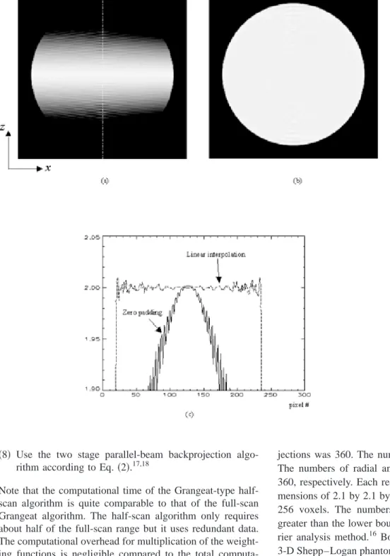
Figure 10 shows the results obtained from the y⫽0 plane of the sphere phantom. The half-scan algorithm cannot pro-duce an exact reconstruction for a general object due to the incompleteness of projection data but in special cases like a sphere phantom this algorithm can achieve exact reconstruc-tion with linear interpolareconstruc-tion. When data in the shadow zone are linearly interpolated from the half-scan data of a sphere, an exact reconstruction of the sphere can be achieved be-cause the radon transform of a perfect sphere is linear.15This exactness seems impossible with other half-scan cone-beam reconstruction algorithms. Nevertheless, this property is de-FIG. 10. Grangeat-type half-scan re-construction of the sphere phantom in the plane y⫽0.共a兲Zero padding;共b兲 linear interpolation, 共c兲 comparative profiles from the identical positions marked by the dashed line in 共a兲. 共Contrast range: 1.90–2.05.兲
sirable in a number of major applications, such as micro-CT studies of spherical specimens.
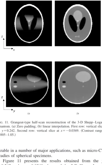
Figure 11 presents the results obtained from the y
⫽0.242 and x⫽⫺0.0369 planes of the 3-D Shepp–Logan phantom. With the zero-padding method, the low-intensity dropaway from the centerplane was found to be more serious than that with the Feldkamp half-scan reconstruction. With the linear interpolation method, this type of artifacts was essentially eliminated.
Figure 12 compares the full-scan and half-scan Grangeat algorithms. Linear interpolation was applied with both algo-rithms. As compared to the Grangeat reconstruction in the full-scan case, little image degradation was visually per-ceived in all the Grangeat-type half-scan reconstructions we performed.
Figure 13 compares Feldkamp-type half-scan reconstruction5 and our Grangeat-type half-scan reconstruc-tion.
IV. DISCUSSIONS AND CONCLUSION
In the writing period of our first draft, it came to our attention that Noo and Heuscher just published a half-scan cone-beam reconstruction paper in an SPIE conference.9The similarity between our work and their paper is that both the groups considered the half-scan cone-beam reconstruction in the Grangeat framework. However, their work is in the fil-tered backprojection framework,10while ours is in the rebin-ning Grangeat framework.7
We believe that both half-scan algorithms are complemen-tary. It seems that data filling mechanism is more flexible in our radon-rebinning framework. Noo and Heuscher sug-gested that the parallel-beam approximation of cone-beam projection data be used to estimate missing data, which is done in the spatial domain. This kind of spatial domain pro-cessing is also allowed in our framework. In addition to the spatial domain approximation, the radon domain estimation, such as linear interpolation, spline interpolation and knowledge-based interpolation, can be done in our work as well. However, in the filtered backprojection frame-work, each frame of cone-beam projection data can be pro-cessed as soon as it is acquired, a desirable property for practical implementation. Clearly, a systematic comparison of the two algorithms is worthy of further investigation.
In conclusion, we have formulated a Grangeat-type half-scan algorithm in the circular half-scanning case. The half-half-scan spans 180° plus two cone angles, allowing exact in-plane reconstruction. The smooth half-scan weighting functions have been designed for the suppression of data inconsistency. Numerical simulation results have verified the correctness and demonstrated the merits of our formulas. This Grangeat-type half-scan algorithm is considered promising for quanti-tative and dynamic biomedical applications of CT and micro-CT. The extension of this work to the helical geometry is being actively pursued.18We will also study other prom-ising reconstruction methods in the future.19–22
ACKNOWLEDGMENTS
We would like to thank Dr. Dominic J. Heuscher共Phillips Medical Systems, Cleveland, Ohio兲 and Dr. Frederic Noo 共Department of Radiology, University of Utah兲for mailing us their SPIE paper.9This work was supported in part by the NIH Grant No. R01 DC03590.
APPENDIX: DERIVATION OF THE GRANGEAT-TYPE HALF-SCAN ALGORITHM
Grangeat found a link between radon data and cone-beam projection data, which is expressed as follows:
R f共nជ兲⫽R
⬘
f共nជ兲 ⫽cos12 s冕
⫺⬁ ⬁ SO SA X f关s共nជ兲,t,共nជ兲兴dt ⫽ 1 cos2 s冕
⫺⬁ ⬁ Xwf关s共nជ兲,t,共nជ兲兴dt. 共A1兲 In the circular full-scan case, there always exist two detector planes from which the radon data can be calculated, except for the shadow zone. The detector planes are specified by the following two equations:1共,,兲⫽⫹sin⫺1
冉
SO sin
冊
, 共A2兲 FIG. 11. Grangeat-type half-scan reconstruction of the 3-D Shepp–Loganphantom.共a兲Zero padding;共b兲linear interpolation. First row: vertical slice at y⫽0.242. Second row: vertical slice at x⫽⫺0.0369.共Contrast range: 1.005–1.05.兲
2共,,兲⫽⫹⫺sin⫺1
冉
SO sin
冊
. 共A3兲 In an ideal situation where data is noise-free and the object is stationary during the rotation, we have1 cos2 s
冕
⫺⬁ ⬁ SO SA Xwf„s共nជ兲,t,1共nជ兲…dt ⫽ 1 cos2 s冕
⫺⬁ ⬁ SO SA Xwf„s共nជ兲,t,2共nជ兲…dt. 共A4兲 Therefore, the radon data can be calculated from either of the detector planes. However, in practice, we should consider the following practical conditions: 共1兲 Projection data contain noise; 共2兲 data from D1 and D2 may be different due to
motion of an object. Hence, we have 1 cos2 s
冕
⫺⬁ ⬁ SO SA X f„s共nជ兲,t,1共nជ兲…dt ⫽ 1 cos2 s冕
⫺⬁ ⬁ SO SA X f„s共nជ兲,t,2共nជ兲…dt. 共A5兲 Considering noise in projection data, we should combine re-dundant data to improve the signal-to-noise ratio. Conse-quently, Eq.共A5兲can be modified to the following: R f共nជ兲⫽
兺
i⫽1 2 i共nជ兲 1 cos2 s ⫻冕
⫺⬁ ⬁ SO SA X f„s共nជ兲,t,i共nជ兲…dt, 共A6兲 where1(nជ)⫹2(nជ)⫽1. To maximize the signal to noise ratio, both1(nជ) and2(nជ) should equal to 1/2.18 How-ever, when motion is significant, one of the solutions to
sup-FIG. 12. Grangeat-type reconstruction of the 3-D Shepp–Logan phantom.共a兲 Full-scan reconstruction;共b兲half-scan reconstruction; 共c兲 comparative pro-files from the identical positions marked by the dashed line in 共a兲. 共Contrast range: 1.005–1.05.兲
press the motion artifacts is to use a half-scan. But in this case, data are not always redundant by a factor of 2. More exactly, there are generally doubly, singly sampled regions, and shadow zones on a meridian plane. Therefore, there exist discontinuities between the adjacent regions. Hence, the smooth weighting functions such as those in Sec. II E are needed to suppress the associated artifacts.
a兲Corresponding address: Seung Wook Lee and Ge Wang, CT/Micro-CT Laboratory, Department of Radiology, University of Iowa, Iowa City, IA 52242. Telephone: 319-384-5616; fax: 319-356-2220; electronic mail: [email protected], [email protected]
1G. Wang, C. R. Crawford, and W. A. Kalender, ‘‘Multirow detector and
cone-beam spiral/helical CT,’’ IEEE Trans. Med. Imaging 19, 817– 821 共2000兲.
2
Y. Liu, H. Liu, Y. Wang, and G. Wang, ‘‘Half-scan cone-beam CT fluo-roscopy with multiple x-ray sources,’’ Med. Phys. 28, 1466 –1471共2001兲.
3D. L. Parker, ‘‘Optimal short scan convolution reconstruction for
fan-beam CT,’’ Med. Phys. 9, 254 –257共1982兲.
4G. T. Gullberg and G. L. Zeng, ‘‘A cone-beam filtered backprojection
reconstruction algorithm for cardiac single photon emission computed tomography,’’ IEEE Trans. Med. Imaging 11, 91–101共1992兲.
5G. Wang, Y. Liu, T. H. Lin, and P. C. Cheng, ‘‘Half-scan cone-beam x-ray
microtomography formula,’’ Scanning 16, 216 –220共1994兲.
6S. Zhao and G. Wang, ‘‘Feldkamp-type cone-beam tomography in the
wavelet framework,’’ IEEE Trans. Med. Imaging 19, 922–929共2000兲.
7
P. Grangeat, ‘‘Mathematical Framework of Cone Beam 3D Reconstruc-tion via the First Derivative of the Radon Transform,’’ in Mathematical
Methods in Tomography, Lecture Notes in Mathematics, edited by G. T.
Herman, A. K. Luis, and F. Natterer共Springer-Verlag, Berlin, 1991兲, pp. 66 –97.
8G. Wang, T. H. Lin, P. C. Cheng, and T. M. Shinozaki, ‘‘A general
cone-beam reconstruction algorithm,’’ IEEE Trans. Med. Imaging 12, 483– 496共1993兲.
9F. Noo and D. J. Heuscher, ‘‘Image reconstruction from cone-beam data
on a circular short-scan,’’ Proc. SPIE 4684, 50–59共2002兲.
10M. Defrise and R. Clack, ‘‘A cone-beam reconstruction algorithm using
shift-variant filtering and cone-beam backprojection,’’ IEEE Trans. Med. Imaging 13, 186 –195共1994兲.
11B. D. Smith, ‘‘Image reconstruction from cone-beam projections:
Neces-FIG. 13. Feldkamp-type half-scan and Grangeat-type half-scan reconstruc-tions. 共a兲 Original phantom 共b兲 Feldkamp-type half-scan reconstruc-tion; 共c兲 Grangeat-type half-scan re-construction,共d兲comparative profiles from the identical positions marked by the dashed line in共a兲.共Contrast range: 1.005–105.兲
sary and sufficient conditions and reconstruction methods,’’ IEEE Trans. Med. Imaging MI-4, 14 –25共1985兲.
12H. K. Tuy, ‘‘An inversion formula for cone-beam reconstruction,’’ SIAM
J. Appl. Math.共Soc. Ind. Appl. Math.兲43, 546 –552共1983兲.
13C. Jacobson, ‘‘Fourier methods in 3D-reconstruction from cone-beam
data,’’ Ph.D. thesis, Linkoeping University, 1996.
14B. D. Smith, ‘‘Computer-aided tomographic imaging from cone-beam
data,’’ Ph.D. thesis, University of Rhode Island, 1987.
15
S. R. Deans, The Radon Transform and Some of its Applications共 Wiley-Interscience, New York, 1983兲.
16S. W. Lee, G. Cho, and G. Wang, ‘‘Artifacts associated with
implemen-tation of the Grangeat formula,’’ Med. Phys. 29, 2871–2880共2002兲.
17
R. B. Marr, C. Chen, and P. C. Lauterbur, ‘‘On two approaches to 3D reconstruction in NMR zeugmatography,’’ in Mathematical Aspects of
Computerized Tomography, Lecture Notes in Mathematics, edited by G.
T. Herman and F. Natterer共Springer-Verlag, Berlin, 1981兲, pp. 225–240.
18
G. Wang and M. W. Vannier, ‘‘Helical CT image noise-analytical re-sults,’’ Med. Phys. 20, 1635–1640共1993兲.
19
S. W. Lee and G. Wang, ’’Grangeat-type helical half-scan CT algorithm for reconstruction of a short object,’’ Med Phys.共submitted兲.
20A. Katsevich, ‘‘Analysis of an exact inversion algorithm for spiral
cone-beam CT,’’ Phys. Med. Biol. 47, 2583–2597共2002兲.
21M. Jiang and G. Wang, ‘‘Convergence of the simultaneous algebraic
re-construction technique共SART兲,’’ IEEE Trans. Image Processing共to ap-pear兲.
22M. Jiang and G. Wang, ‘‘Convergence studies on iterative algorithms for