A Multiview Approach for Intelligent Data
Analysis based on Data Operators
Yaohua Chen and Yiyu Yao
Department of Computer Science, University of Regina Regina, Saskatchewan, Canada S4S 0A2
E-mail: {chen115y, yyao}@cs.uregina.ca
Abstract
Multiview intelligent data analysis explores data from different perspectives to re-veal various types of structures and knowledge embedded in the data. Each view may capture a specific aspect of the data and hence satisfy the needs of a particu-lar group of users. Collectively, multiple views provide a comprehensive description and understanding of the data. In this paper, we propose a multiview framework of intelligent data analysis based on modal-style data operators. The classes of the data operators include basic set assignment, sufficiency, dual sufficiency, necessity and possibility operators. They demonstrate various types of data relationships and characterize various features and granulated views of the data. It is shown that different structures of the data can also be constructed based on the different data operators.
Key words: Multiview, Intelligent Data Analysis, Modal-style Data Operators, Concept Lattice, Granular Computing.
1 Introduction
Huge data sets and various data types lead to new types of problems and require the development of new types of techniques for modern intelligent data analysis [21]. An important objective of intelligent data analysis is to reveal and indicate diverse non-trivial features or views of a large amount of data. Many techniques and models in data mining, machine learning, pattern recognition, statistics, and other fields have been proposed. Each technique or model focuses on one particular view of the data and discovers a specific type of knowledge embedded in data.
In this paper, we propose a multiview approach that provides a unified frame-work for integrating multiple views of intelligent data analysis. It is easy to
know that an integrated and unified framework that allows a multiple view approach on the understanding, computation, and interpretation of data pro-vides not only a platform to explore different aspects of the data, but also a tool to integrate many techniques of intelligent data analysis.
Modal-style data operators can be used to define, represent and analyze vari-ous types of data relations and structures [6,53]. Therefore, these modal-style data operators can provide a unified way to examine, characterize and con-struct different types of knowledge. In this paper, the multiview approach are defined based on modal-style data operators in a formal context.
The rest of the paper is organized as follows. In the next section, discussions about motivations and some related works are provided. Section 3 introduces formal contexts and modal-style data operators. In Section 4, we show that these data operators can be used to define different relations and granular structures of a universe. Section 5 examines several types of hierarchical struc-tures defined based on the modal-style data operators. These granular and hierarchical structures are always be viewed as different types of knowledge embedded in the data set [11,6,39,53]. The conclusion of this study is given in Section 6.
2 Motivations and Related Work
In this section, we give motivations of this proposed research work and discuss some related work.
2.1 Motivations
Many techniques and models have been proposed for intelligent data analysis. In data mining, association rule mining is to detect the association relationship between two sets of items [1]. An association rule expresses that a customer buying one set of items tends to buy another set of items. Association rules can be considered as a description of association relationships among the data. In machine learning and pattern recognition, the techniques of classification and cluster learning focus on prediction of future data, plan future action, etc. [16,23,28]. They can be viewed as seeking for different types of relation-ships among the data. Each technique is designed with respect to the specific properties of the relationships [23]. Some techniques are proposed to detect the degree of similarity or commonality, such as template matching models [5,19], nearest neighbor models [13], kernel density models [40]. Some techniques are designed to construct decision boundaries or a partition based on commonality
of entities, such as decision tree [9,44,45], neural networks [2,3,35], and sup-port vector machine [48]. Bayesian networks have been proposed and studied to classify entities into the class with respect to the maximum posterior proba-bilities of the entities [23,41]. Clustering is to directly partition unlabeled data based on some properties of the relationships among the data [22,27]. Many types of relationships can be used to determine which class the entities belong to, such as similarity, correlation, dependency, association, and so on [4]. Many techniques for data clustering have been proposed, such as K-means cluster-ing [33], hierarchical clustercluster-ing [26,46,49], nearest neighbor clustercluster-ing [32], and density based clustering [15].
Most proposed techniques and models overemphasize the automation and effi-ciency of the data analysis systems, but neglect the effectiveness of the systems. To a large extent, the effectiveness determines the quality of the systems and satisfiability of human users [38]. There are two aspects of the effectiveness of data analysis systems. On the one hand, from a system or data set, a user is able to explore different types of knowledge, different features of data, and different interpretations of data with respect to different techniques, models, and user preferences. On the other hand, multiple aspects of data understand-ing, multiple angles of data summarizations or data descriptions, and multiple types of discovered knowledge are useful for satisfying a wide range of needs of a large diversity of users.
Therefore, a system providing multiple views of a data set is crucial and nec-essary for intelligent data analysis. In this paper, we propose an approach for multiview intelligent data analysis and demonstrate that one can discover different types of knowledge from a data set.
Modal-style data operators have been studied by many researchers for in-telligent data analysis [11,14,17,18,50,51,54,55]. These data operators can be used to define, represent and analyze various types of relations and struc-tures embedded in the data, which are generally viewed as different types of knowledge [6,53]. We use these modal-style data operators defined based on a formal context to examine, characterize and construct different types of data structures and knowledge.
For example, classifications of the universe induced by the relations produce various types of granular structures of the universe. Two types of structures, partition and covering, can be analyzed and discussed with respect to different modal-style data operators. Some hierarchical structures embedded in the data can also be defined based on modal-style data operators. Each hierarchical structure explores a particular organization of the data.
2.2 Related Work
Multiple view strategies and approaches have been proposed and studied in many fields, including social sciences, software design, machine learning, and data analysis [7,8,24,34,62]
Jeffries and Ransford argued that the study of social stratification should not focus on isolated and fragmented views, but holistic and unified views [24]. The study of social stratification identifies and investigates the characteristics of social societies. It focuses primarily on the hierarchies of social classes. The traditional single hierarchy approach based on social classes limits one’s un-derstanding of the complexities of modern societies. The authors proposed a multiple hierarchy model to integrate class, ethnicity, gender, and age social inequality hierarchies. These four hierarchies are considered as separated but interrelated. The study shows that a multiple hierarchy approach could in-crease one’s understanding and be more comprehensive and valid for studying social inequality.
Belkhouche and Lemus-Olalde studied the formal foundations of an abstract interpretation of multiple views at the software design stage [7,8]. In the pro-cess of modeling a system, the designer always generates a set of designs, such as functional, behavioral, structural and data designs. Each design focuses on a view that describes a subset of relevant features of a system and is ex-pressed by one or more notations. Different designs show different viewpoints of the system. Functional designs describe what the system does in terms of its tasks. Behavioral designs describe the causal links between events and system responses during execution. Structural designs concern the essentially static aspects of the system. Data designs concern the data used in system and relationships between them. The authors argued that a multiple view anal-ysis framework can be used to systematically compare, identify and analyze the discrepancies among different views, enhance design quality and provide a multi-angled understanding of a problem or a project.
Several researchers proposed frameworks of multistrategy learning to integrate a wide range of learning strategies [34]. They argued that the research on multistrategy learning systems is significantly relevant to study on human learning since human learning is clearly multistrategy. Multistrategy systems have a potential to be more versatile and more powerful to solve a much wider range of learning problems than monostrategy systems. Some conceptual frameworks, such Inferential Theory of Learning and Plausible Justification Trees, are proposed to investigate the logical capabilities and relationships of various learning methods and processes. Based on the proposed frameworks, methodologies and applications for multistrategy task-adaptive learning have been developed [34].
Zhonget al.proposed an approach of multiple aspect analysis of human brain data for investigating human multiperception mechanism [61,62]. By using different methods and measurements, they can obtain various types of human brain data. They observed that each type of data extracted by a particular method or measure matches human ability in a specific aspect. Each approach to analyze the obtained data is also processed with respect to the specific state or the related part of a stimulus. They argued that every method or model of data acquisition and analysis has its own strength and weakness. Thus, designing psychological and physiological experiments for obtaining various data from human multiperception mechanism and analyzing such data from multiple aspects for discovering new models of human multiperception are the key issues. They proposed a framework of data-mining grid for multiple human brain data analysis by cooperatively using cognitive and data-mining techniques, and attempted to change the perspective of cognitive scientists from a single type of experimental data analysis toward a holistic view. In data mining, some researchers have already recognized that integration of association rule mining and classification can produce a more accurate clas-sifier [31,58,63]. Approaches on integrating clustering and classification tech-niques can also achieve better classification or clustering results [20,25,29,60].
3 Formal Contexts and Modal-style Data Operators
In this section, definitions for formal contexts and modal-style data operators are given. Some connections between modal-style data operators are investi-gated.
3.1 Formal Contexts
We assume that a data set is given in terms of a formal context [50] or a binary table [39]. It provides a convenient way to describe a finite set of objects by a finite set of attributes. For simplicity, we only consider a finite set of objects and a finite set of attributes in this paper. The results may not be true for the infinite cases.
Let U and V be any two finite sets. Elements of U are called objects and
elements of V are called attributes or properties. The relationships between
objects and attributes are described by a binary relation R between U and
V, which is a subset of the Cartesian product U ×V. For a pair of elements
x ∈ U and y ∈ V, if (x, y) ∈ R, written as xRy, we say that x has the
Table 1
A Formal Context From [47]
PO LM SM VM VC AT CS DM IC AD 1. Picture Completion √ √ √ √ 2. Picture Arrangement √ √ √ √ √ √ 3. Block Design √ √ √ √ √ 4. Object Assembly √ √ √ √ √ 5. Digit Symbol √ √ √
PO: Perceptual Organization,LM: Long-term Memory,SM: Short-term Memory, VM: Visual Memory,VC: Visual-motor Coordination,AT: Abstract Thought, CS: Common Sense,DM: Decision Making,IC: Intellectual Curiosity,AD: Attention to Detail. called a formal context [17,50] or a binary information table [39]. In general, a multi-valued formal context can be transformed into a binary formal context through scaling [17]. That is, every information table can be represented by a formal context [10].
Example 1 Table 1 is an example of a formal context taken from [47]. The attributes describe the abilities of human brain. The objects represent the re-alistic actions that need human brain to perform. A binary relation determine which actions should be performed by which abilities. Thus, objects and at-tributes in a formal context are described and determined by each other based on the binary relation.
Based on the binary relation R, we can associate a set of attributes with an
object. An object x∈U has the set of attributes:
xR={y∈V |xRy} ⊆V.
The set of attributes xR can be viewed as a description of the object x. In
other words, objectxis described or characterized by the set of attributesxR.
Similarly, an attributey is possessed by the set of objects:
Ry={x∈U |xRy} ⊆U.
By extending these notations, we can establish relationships between sets of objects and sets of attributes. This leads to two types of data operators, one
from 2U to 2V and the other from 2V to 2U, where 2U and 2V are the power
3.2 Modal-style Data Operators
With a formal context, we can define different types of modal-style data op-erators. Each of them leads to a different type of rules summarizing the rela-tionships between objects and attributes.
Basic Set Assignments: For a set of objects A⊆U and a set of attributes
B ⊆ V, we can define a pair data operators, b : 2U → 2V and b : 2V → 2U,
called basic set assignments, as follows [52]:
Ab ={y∈V |Ry =A},
Bb ={x∈U |xR=B}.
For simplicity and clarity, the same symbol is used for both operators. The
operators b associate a set of objects with a set of attributes and a set of
attributes with a set of objects. They satisfy the following properties: for A, A1, A2 ⊆U,
(b1) ∅b =∅,
(b2) V =[{Ab |A⊆U},
(b3) A1 6=A2 =⇒Ab1 ∩Ab2 =∅.
Property (b1) states that the assigned set for an empty set is the empty set. It should be pointed out that property (b1) holds only if the formal context
satisfies the condition: Ry 6= ∅, for all y ∈ V. Property (b2) shows that the
union of assigned sets of attributes for all subsets of objects is the entire set
of attributes V. Property (b3) means the assignments for different subsets of
objects are distinct and non-overlapping. Properties (b2) and (b3) hold for any binary relation. The property (b1) holds if an object must have an attribute or an attribute must be possessed by an object.
Sufficiency Operators: For a set of objects A ⊆ U and a set of attributes
B ⊆ V, we can define a pair data operators, ∗ : 2U → 2V and ∗ : 2V → 2U,
called sufficiency operators, as follows [17,50]:
A∗={y∈V |A⊆Ry} = \ x∈A xR, (1) B∗={x∈U |B ⊆xR} = \ y∈B Ry. (2)
The same symbol is used for both operators. By definition, {x}∗ = xR is
the set of attributes possessed by the object x, and {y}∗ = Ry is the set of
objects having attribute y. For a set of objects A, A∗ is the maximal set of
properties shared by all objects in A. Similarly, for a set of attributes B, B∗
is the maximal set of objects that have all attributes inB.
Dual Sufficiency Operators: For a set of objects A ⊆ U and a set of
attributes B ⊆ V, we can define a pair data operators, # : 2U → 2V and
#: 2V →2U, called dual sufficiency operators, as follows [55]:
A#={y∈V |A∪Ry 6=U},
B# ={x∈U |B∪xR6=V}.
The same symbol is again used for both operators. For a subset A ⊆ U, an
attribute in A# is not possessed by at least one object not in A.
The following properties hold for the sufficiency operators [17,50]: forA, A1, A2 ⊆
U, (s1) ∅∗ =U, (s2) A∗ =Ac#c, (s3) A∗∗∗ =A∗, (s4) A1 ⊆A2 =⇒A∗1 ⊇A∗2, (s5) (A1∪A2)∗ =A∗1∩A∗2.
where Ac presents the complement of the set ofA. The dual sufficiency
oper-ators have the following properties [55]: for A, A1, A2 ⊆U,
(d1) U# =∅,
(d2) A#=Ac∗c,
(d3) A###=A#,
(d4) A1 ⊆A2 =⇒A#1 ⊆A#2,
(d5) (A1∩A2)#=A#1 ∪A#2 ,
The properties (s1) and (d1) mean that the operation∗ on the empty set will
be the universe, and the operation # on the universe will be the empty set.
The properties (s2) and (d2) show that the operators ∗ and # are dual to
each other. Property (s4) shows that the operator ∗ is monotonic decreasing
with respect to set inclusion while property (d4) shows that the operator #
is monotonic increasing. Similar properties hold for the operators ∗ and # on
A pair of dual mappings, ∗ : 2U → 2V and ∗ : 2V → 2U, is indeed a Galois
connection between two partially ordered sets h2U,⊆i and h2V,⊆i [14,51].
Necessity Operators: For a set of objects A ⊆ U and a set of attributes
B ⊆ V, we can define a pair data operators, 2 : 2U → 2V and 2 : 2V → 2U,
called necessity operators, as follows [14,18,54,55]:
A2 ={y∈V |Ry⊆A},
B2 ={x∈U |xR ⊆B}.
The same symbol is used for both operators. By definition, an object having
an attribute in A2 is necessarily in A. The operators are referred to as the
necessity operators.
Possibility Operators: For a set of objects A ⊆ U and a set of attributes
B ⊆ V, we can define a pair data operators, 3 : 2U → 2V and 3 : 2V → 2U,
called possibility operators, as follows [14,18,54,55]:
A3={y∈V |Ry∩A6=∅} = [ x∈A xR, B3={x∈U |xR∩B 6=∅} = [ y∈B Ry.
The same symbol is again used for both operators. An object having an
at-tribute in A3 is only possibly in A. The operators are referred to as the
possibility operators.
The necessity operators have the following properties [54]: for A, A1, A2 ⊆U,
(n1) U2 =V,
(n2) A2 =Ac3c,
(n3) A1 ⊆A2 =⇒A21 ⊆A22,
(n4) (A1∩A2)2 =A21 ∩A22.
The possibility operators have the following properties [54]: forA, A1, A2 ⊆U,
(p1) U3 =V,
(p2) A3=Ac2c,
(p3) A1 ⊆A2 =⇒A31 ⊆A32,
The properties (n1) and (p1) state that the universe U are mapped to the
entire set of attributeV. The properties (n2) and (p2) show that the operators
2 and 3 are dual to each other. The properties (n3) and (p3) say that these
two operators are monotonic increasing. Property (n4) states that the operator
2 is distributive over set intersection ∩, while property (p4) states that the
operator 3 is distributive over set union ∪.
3.3 Connections between Data Operators
Since the modal-style data operators are defined based on the binary relation
R of a formal context, there exist connections among these modal-style data
operators [55]. In terms of the basic set assignment, we can re-express operators
∗, 2 and 3 as:
(1) A∗ =[{Xb |X ⊆U, A⊆X},
(2) A#=[{Xb |X ⊆U, X∪A6=U},
(3) A2 =[{Xb |X ⊆U, X ⊆A},
(4) A3=[{Xb |X ⊆U, A∩X 6=∅}.
In other words, the sufficiency, dual sufficiency, necessity and possibility
oper-ations on a setAcan be expressed by a union of some particular basic assigned
sets for A.
Conversely, one can re-express operator b by using operators ∗ and 2 as:
(5) Ab =A∗∩A2,
(6) Ab =A∗−[{X∗ |A⊂X},
(7) Ab =A2−[{X2 |X ⊂A}.
The basic set assignment on a set A is the intersection of sufficiency and
necessity operations on A. Moreover, for a set A, the result of removing the
union of the sufficiency operations on all proper subset ofAfrom the sufficiency
operation on set A is the basic set assignment on A. Similarly, the result of
removing the union of the necessity operations on all proper superset of A
from the necessity operation on set A is also the basic set assignment on A.
Example 2 A simple example is provided to illustrate the semantic meanings of each modal-style data operator.
The formal context in Table 1 describes the relationships between actions and human brain abilities. In this table, the objects represent the actions, such
as picture completion, picture arrangement, block design, object assembly and digit symbol. The attributes represent the brain abilities needed to complete the actions.
The relation xRy, where x ∈ U and y ∈ V is interpreted as “Action x is
performed by using the brain ability y”. Suppose Adenotes a behavior, a set of
actions, and y denotes a brain ability. The data operators can be interpreted
as follows:
y∈Ab ⇐⇒The ability y is needed for performing exactly the set of actions A,
y∈A∗ ⇐⇒The ability y is sufficient to perform all actions in A,
y∈A# ⇐⇒Not all actions in Ac can be performed by y,
y∈A2 ⇐⇒The actions performed by using y are necesarily in A,
y∈A3 ⇐⇒The ability y is possibly used to perform some action in A.
SupposeB denotes a set of abilities, and x denotes an action. The data
oper-ators can be interpreted as follows:
x∈Bb ⇐⇒ The action x is exactly performed by all abilities in B,
x∈B∗ ⇐⇒ The action x is sufficiently performed by all abilities in B,
x∈B# ⇐⇒ Not all abilities in Bc can perform x,
x∈B2 ⇐⇒ The ability to perform the action x is necessarily in B,
x∈B3 ⇐⇒ The action x is possibly performed by some ability in B.
Based on these modal-style data operators, one can compose new data oper-ators to express various features of the data. In the next two sections, we will show that the modal-style data operators can not only be used to define vari-ous types of relations between objects and induced granular structures of the universe, but also be used to define different types of hierarchical structures of the data.
4 Granular Structures of the Universe
In this section, we investigate various relations between objects and granular structures induced by the relations based on modal-style data operators.
4.1 Granulation and Granular structure
Granular computing has emerged as a multi-disciplinary study of problem solving and information processing [6,30,36,39,42,43,53,59]. It provides a gen-eral, systematic and natural way to analyze, understand, represent, and solve real world problems. Granulation and granular structure of the universe are fundamental issues in granular computing. Granular structures are used to classify and characterize the data [53,59].
Granulation deals with the grouping of individual elements of a universe into classes or sets called granules. A family of granules provides a granulated view of the universe. Elements in a granule are grouped together by indistinguisha-bility, similarity, proximity or functionality [36,59]. There are both semantics and algorithmic aspects of granulation. A semantic interpretation explains why two objects are put into the same granule and an algorithm determines how two objects are related with each other. The granules in a granulated view can be either disjoint or overlapping and are regarded as a level of un-derstanding the subject matter of the study. The different granulated views can be viewed as different granular structures of a universe. Generally, there are two types of granulations, and the corresponding granular structures are partition and covering of the universe.
A simple way for the granulation of a universeU is through a binary relation<
onU. A binary relation<over a universeU is a subset of the Cartesian product
U×U. Based on<, a 1-neighborhood system of objects can be constructed [56].
For two objectsx, x0 ∈U, ifx<x0, we say thatxis a predecessor of x0, andx0 is
a successor ofx. The set of predecessors ofxis called predecessor neighborhood
and denoted by<x={x0 ∈U |x0<x}, and the set of successors of xis called
successor neighborhood and denoted by x< = {x0 ∈ U | x<x0}. A binary
relation < on U is called an equivalence relation if it is reflexive, symmetric
and transitive:
Reflective : for all x∈U, x<x,
Symmetric : for all x∈U, x<x0 =⇒x0<x,
Transitive : for allx∈U, [x<x0, x0<x00] =⇒x <x00.
An equivalence relation partitions the universe U into a family of disjoint
subsets. This partition of the universe is denoted by U/E [57]. The elements
of the partitionU/E are called granules and satisfy the following properties:
(I) Xi∩Xj =∅, where Xi, Xj ∈U/E, i6=j,
Conversely, given a partition of the universe, we can construct uniquely an equivalence relation that produces the same partition. There is a one-to-one correspondence between partitions of a universe and equivalence relations on the universe.
The notion of a covering of a universe is a generalization of a partition by
removing the non-overlapping condition (I). Let C be a family of subsets of
U. It is called a covering ofU if the following condition holds:
(III) U =[{X |X ∈C}.
Unlike the case of equivalence relations, we cannot establish a one-to-one cor-respondence between coverings and a class of binary relations. Nevertheless,
for a reflexive relation <, the family of successor neighborhoods{x< |x∈U}
is a covering of the universe.
The binary relations between objects in turn can induce different granular structures. Modal-style data operators can be used to define different relations between objects.
4.2 Granular Structures Induced by Modal-style Operators
Many types of binary relations between objects have been studied [37,56]. The relations between objects can be defined based on the relations between their descriptions, i.e. sets of attributes. In other words, one can use the relations
between objects and attributes, R : U ×V, to define the relations between
objects, <:U ×U. In this paper, we consider four types of relations:
equiva-lence relation, partial order relation, similarity relation and negative similarity relation.
Equivalence Relation: Two objects may be viewed as being equivalent if they have the same description, i.e. they share the same set of attributes [39].
An equivalence relation can be defined by: forx, x0 ∈U,
x ≡U x0 ⇐⇒xR =x0R.
With equivalence relation≡U, an object has the same predecessor and
succes-sor neighborhood. For an objectx∈U, the set of objects that are equivalent
tox is called an equivalence class of x and defined by:
={x0 ∈U |x ≡U x0},
=x≡U,
= [x].
The equivalence classes can be re-expressed by using modal-style data
opera-tors. In a formal context (U, V, R), for an object x∈ U, its equivalence class
can be re-expressed by:
[x] ={x0 ∈U |x0 ≡U x},
={x0 ∈U |xR =x0R},
={x0 ∈U |x0R ={x}∗},
={x}∗b.
The objects in [x] are considered to be indistinguishable fromx. One is
there-fore forced to consider [x] as a whole. In other words, under an equivalence
relation, equivalence classes are the smallest non-empty observable,
measur-able, or definable subsets of U.
A subset of objects A⊆U is called a focal set of objects if Ab 6=∅. Similarly,
we can define a focal set of attributes. By the properties of the basic set
assignment, the partition U/E is indeed the assignments of the focal sets of
attributes:
U/≡U={Yb 6=∅ |Y ⊆V}.
This can be easily seen from the fact that each objectx∈Yb possesses exactly
the set of attribute Y.
Similarity Relation: If two objects x and x0 have some overlapping at-tributes, they are regarded as being similar to each other. This type of relation
is defined by [37]: forx, x0 ∈U,
x ≈U x0 ⇐⇒x0R∩xR6=∅.
The relation is reflexive and symmetric, but not necessarily transitive.
Based on the similarity relation≈U, for an object, its predecessor and successor
neighborhoods are the same because of the symmetric property of ≈U. In a
formal context (U, V, R), for an objectx∈U, the≈U predecessor and successor
neighborhood are given by:
≈Ux=x≈U,
={x0 ∈U |x ≈
={x0 ∈U |x0 ≈U x},
={x0 ∈U |x0R∩xR6=∅},
={x}33.
The objects in {x}33 must share some attributes of x. The union of all such
sets of objects is the universe U, that is, U = S{{x}33 | x ∈ U}. Thus, the
family of all sets of objects induced by similarity relation ≈U is a covering of
the universe U.
Negative Similarity Relation: For two objects x and x0, if the union of their attributes is not the whole set of attributes, we can consider them as
being negatively similar [37]. This type of relation is defined by: forx, x0 ∈U,
x ³U x0⇐⇒xRc∩x0Rc6=∅,
⇐⇒xR∪x0R6=V,
whereRcis the complement of the relationR. The negative similarity relation
is only symmetric.
For the negative similarity relation ³U, the predecessor and successor
neigh-borhoods for an object are the same. For an objectx∈U, the³U predecessor
and successor are:
³Ux=x³U, ={x0 ∈U |x ³U x0}, ={x0 ∈U |x0 ³ U x}, ={x0 ∈U |xR∪x0R6=V}, ={x}∗#.
For an object x0 in{x}∗#, there must exist at least one attribute that is not
possessed by both x and x0. The family of all sets of objects {x}∗# induced
by the negative similarity relation ³U may not be necessarily a partition or
covering of the universeU.
Partial Order Relation: A partial order relation on objects can be defined
based on set inclusion: for x, x0 ∈U,
x ¹U x0 ⇐⇒xR ⊆x0R.
It is reflexive and transitive.
A partial order relation is not necessarily symmetric. In this case, we have different predecessor and successor neighborhoods for an object. For an object
x¹U={x0 ∈U |x ¹U x0},
={x0 ∈U |xR⊆x0R},
={x0 ∈U | {x}∗ ⊆x0R},
={x}∗∗.
For an object x∈U, the ¹U predecessor neighborhood is given by:
¹Ux={x0 ∈U |x0 ¹U x},
={x0 ∈U |x0R ⊆xR},
={x0 ∈U |x0R ⊆ {x}3},
={x}32.
The set {x}∗∗ is the maximal set of objects that have all attributes in {x}∗.
In other words, any objects in {x}∗∗ has at least all attributes of x. In fact,
each set {x}∗∗ is the extension of an object concept in formal concept
anal-ysis [17,50]. The union of all such sets of objects is the universe U, that is,
U =S{{x}∗∗ | x ∈ U}. Thus, the family of all sets of objects {x}∗∗ induced
by the partial order relation ¹ is a covering the universe U. The set {x}32
is the maximal set of objects whose attributes are subsets of {x}3. In other
words, any object in {x}32 has at most all attributes of x. The union of all
such sets of objects is the universe U, that is, U =S{{x}32 |x ∈U}. Thus,
the family of all sets of objects {x}32 induced by the partial order relation
¹U is a covering the universe U.
4.3 Connections between Granular Structures
These types of data operators induce different types of granulated views of the universe. They can be considered as different types of strategies to divide the universe or classify the objects.
The connections among various types of granular structures can be established based on the connections of the data operators. In fact, the equivalence classes can be used to re-express other types of sets of objects.
{x}∗∗=[{[x0]|xR⊆x0R},
{x}∗#=[{[x0]|xR∪x0R 6=V},
{x}32=[{[x0]|xR⊇x0R},
Similar to the granulations on objects, we can also define the various granu-lations on attributes by using modal-style data operators. The detailed defi-nitions and formulas of these granulations on attributes are given in the Ap-pendix.
5 Hierarchical Structures Embedded in Data
In the classical view, a concept is determined by its extension and intention. The extension consists of all objects belonging to the concept. The intension includes all attributes that are used to measure the objects belonging to the concept. A pair of extension and intention is considered as a representation of a concept. Lattice theory provides a proper vocabulary for hierarchical structures and can be applied to construct concept lattices [17,50,54,55]. In this section, the modal-style data operators are examined to construct dif-ferent types of concept lattices. Several types of concept lattices are derived from a same formal context and reflect various features of the data and to represent a diversity of knowledge embedded in the data.
5.1 Class-oriented Formal Concept Lattice
An equivalence relation between objects can induce a partition of the universe. Each element in the partition is called an elementary definable set [39]. One can construct a definable set by taking a union of some equivalence classes. The
family of all definable sets on the universe U is an σ-algebra σ(U/≡U) ⊆2U
with basisU/≡U, where 2U is the power set ofU [57]. The following properties
hold: (E1) ∅ ∈σ(U/≡U), (E2) U ∈σ(U/≡U), (E3) X ∈σ(U/≡U)⇒Xc∈σ(U/≡U), (E4) A1, A2 ∈σ(U/≡U)⇒A1∩A2 ∈σ(U/≡U), (E5) A1, A2 ∈σ(U/≡U)⇒A1∪A2 ∈σ(U/≡U).
The properties (E1) and (E2) state that the empty set ∅ and the universe
U are in σ(U/≡U). The properties (E3) - (E5) express that the complement,
intersection and union of some definable sets in σ(U/≡U) are still definable
sets in σ(U/≡U). In other words, σ(U/≡U) is closed under set complement,
intersection and union operations. Similarly, the family of all definable sets on
Example 3 In Table 1, the equivalence classes over the universe of objects are:
[1] ={1}, assigned to the focal set {P O, LM, V M, AD},
[2] ={2}, assigned to the focal set {P O, AT, CS, DM, IC, AD},
[3] = [4] ={3,4}, assigned to the focal set {P O, V C, AT, DM, AD},
[5] ={5}, assigned to the focal set {SM, V M, V C}.
The equivalence classes over the universe of attributes are:
[P O] = [AD] = {P O, AD}, assigned to the focal set {1,2,3,4},
[AT] = [DM] = {AT, DM}, assigned to the focal set {2,3,4},
[CS] = [IC] ={CS, IC}, assigned to the focal set {2},
[LM] ={LM}, assigned to the focal set {1},
[SM] ={SM}, assigned to the focal set {5},
[V M] ={V M}, assigned to the focal set {1,5},
[V C] ={V C}, assigned to the focal set {3,4,5}.
A pair (A, B), A ⊆ U, B ⊆ V, is called a class-oriented formal concept if
A ∈ σ(U/≡U)) and B = A∗. The set of objects A is called the extension of
the concept (A, B), and the set of attributesB is called the intension.
For two class-oriented concepts (A1, B1) and (A2, B2), we say that (A1, B1) is
a sub-concept of (A2, B2), and (A2, B2) is a super-concept of (A1, B1), if and
only if A1 ⊆A2.
The family of all class-oriented formal concepts forms a complete lattice called class-oriented formal concept lattice. This lattice gives a hierarchical structure
of the elements in σ(U/≡U) and their corresponding attributes. The meet ∧
and the join ∨ are defined by:
(A1, B1)∧(A2, B2) = ((A1∩A2),(A1∩A2)∗), (A1, B1)∨(A2, B2) = ((A1∪A2),(B1∩B2)).
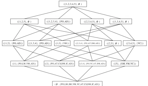
Example 4 The lattice derived from Table 1 is illustrated in Figure 1 in which each rectangle represents a class-oriented formal concept, i.e., a definable set
in the system ofσ(U/≡)and its correspondent attributes. The lines associating
the rectangles is considered as the partial order relations between class-oriented formal concepts.
({1,2,3,4,5},ø )
({1,2,5},ø ) ({1,2,3,4}, {P O ,AD }) ({2,3,4,5},ø ) ({1,3,4,5},ø )
({1,2}, {P O ,AD }) ({1,3,4}, {P O ,AD }) ({1,5}, {VM }) ( {2 ,3 ,4 }, {P O ,A T ,D M ,A D }) ({2,5},ø ) ({3,4,5}, {VC})
({1}, {P O ,LM ,VM ,A D }) ({2}, {P O ,A T ,CS,D M ,IC,A D }) ( {3 ,4 }, {P O ,VC ,A T ,D M ,A D }) ({5}, {S M,VM,VC})
(ø , {P O ,LM ,SM ,VM ,VC,A T ,CS,D M ,IC,A D })
Fig. 1. A Class-oriented Formal Concept Lattice
5.2 Formal Concept Lattice
Wille and Ganter use efficiency operators to define a lattice of formal
con-cepts [17,50]. A pair (A, B), A ⊆ U, B ⊆ V, is called a formal concept if
A = B∗ and B = A∗. The set of objects A is referred to as the extension of
the concept (A, B), and the set of attributesY is referred to as the intension.
Objects inAshare all attributes B, and only attributes in B are possessed by
all objects in A.
For two formal concepts (A1, B1) and (A2, B2), we say that (A1, B1) is a
sub-concept of (A2, B2), and (A2, B2) is a super-concept of (A1, B1), if and only if
A1 ⊆A2, or equivalently, if and only if B2 ⊆B1.
The family of all formal concepts is a complete lattice called a formal concept
lattice [17,50]. The meet∧and the join∨in formal concept lattice are defined
by:
(A1, B1)∧(A2, B2) = (A1∩A2,(B1∪B2)∗∗), (A1, B1)∨(A2, B2) = ((A1∪A2)∗∗, B1∩B2).
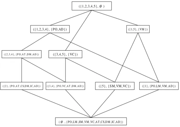
Example 5 Figure 2 is the formal concept lattice formed based on Table 1. Each rectangle represents a formal concept in the lattice. Lines between rect-angles represent the partial order relations between the concepts.
({1,2,3,4,5},ø ) ({1,2,3,4}, {P O ,AD }) ({1,5}, {VM }) ( {2 ,3 ,4 }, {P O ,A T ,D M ,A D }) ({3,4,5}, {VC}) ({1}, {P O ,LM ,VM ,A D }) ( {2 }, {P O ,A T ,C S,D M ,I C ,A D }) ( {3 ,4 }, {P O ,VC ,A T ,D M ,A D }) ({5}, {S M,VM,VC}) (ø , {P O ,LM ,SM ,VM ,VC,A T ,CS,D M ,IC,A D })
Fig. 2. A Formal Concept Lattice
The properties of the operator∗∗ are: for A, A
1, A2 ⊆U,
(SI) U∗∗ =U,
(SII) A⊆A∗∗,
(SII) A∗∗ =A∗∗∗∗,
(SIV) A1 ⊆A2 =⇒A∗∗1 ⊆A∗∗2 .
Property (SI) states that the operation∗∗on the universeUwill be the universe
itself. Property (SII) and (SIV) mean that ∗∗ is a monotonically increasing
operator. Property (SIII) shows that∗∗is a idempotent operator. The operator
∗∗ : 2V → 2V is a closure operator on 2V and has similar properties of the
operator ∗∗: 2U →2U over the universe U.
Let (U,∗∗) denote the family of sets (U,∗∗) ={A∗∗ |A⊆U}. In fact, (U,∗∗)⊆
2U containing the universeU is the set of the extensions of all formal concepts.
The system (U,∗∗) is closed under the operator∗∗and set intersection operator,
but not set union operator. That is, the system (U,∗∗) is a closure system
defined by the following properties [12]:
(S1) U ∈(U,∗∗),
(S2) A1, A2 ∈(U,∗∗) =⇒A1 ∩A2 ∈(U,∗∗).
(U,∗∗) = {A∗∗ = A | A ⊆ U}. Furthermore, for a non-empty set A ∈ (U,∗∗)
and the corresponding formal concept (A, A∗), we have [17]:
(A, A∗) = _{({x}∗∗,{x}∗)|x∈A}.
That is, {x}∗∗ can be used to re-express the sets in the system (U,∗∗). The
whole system (U,∗∗) can be generated by the sets of {x}∗∗, x ∈ U. In fact, a
pair ({x}∗∗,{x}∗), x ∈ U, is a formal concept called an object concept [17].
{x}∗∗ is the extension of an object concept. A formal concept in the lattice
can be generated, composed or re-expressed by some object concepts. In other words, the whole formal concept lattice can be generated by object concepts. 5.3 Dual Formal Concept Lattice
Similar to the efficiency operators for formal concept lattice, the dual efficiency
operators can be used to define a lattice of dual formal concepts. A pair (A, B),
A ⊆U, B ⊆V, is called a dual formal concept if A =B# and B =A#. The
set of objectsA is referred to as the dual extension of the concept (A, B), and
the set of attributes Y is referred to as the dual intension. It can be easily
seen that a pair (A, B) is a dual formal concept if and only if (Ac, Bc) is a
standard formal concept. For a dual concept (A, B), only objects not in A
share all attributes not in B, and only attributes not in B are possessed by
all objects not in A.
For two dual formal concepts (A1, B1) and (A2, B2), we say that (A1, B1) is
a sub-concept of (A2, B2), and (A2, B2) is a super-concept of (A1, B1), if and
only if A1 ⊆A2, or equivalently, if and only if B2 ⊆B1.
The family of all dual formal concepts forms a complete lattice called dual
formal concept lattice. The meet ∧ and the join ∨ in dual formal concept
lattice are defined by:
(A1, B1)∧(A2, B2) = ((A1∩A2)##,(B1∪B2)), (A1, B1)∨(A2, B2) = ((A1∪A2),(B1∩B2)##).
Because of the property of duality of the operators∗ and#, one can re-express
one operator with the other operator as # =c∗c and hence ## =c∗∗c. In other
words, a dual formal concept can be obtained by taking the set complement of the extension and intention of the formal concept.
Example 6 A dual formal concept lattice derived from Table 1 is illustrated in Figure 3. Each rectangle represents a dual formal concept. A line describes
({1,2,3,4,5},ø )
({5}, {LM ,SM ,VM ,VC,A T ,CS,D M ,IC}) ( {2 ,3 ,4 }, {P O ,L M ,SM ,VC ,A T ,C S,D M ,I C ,A D })
({1,5}, {LM,S M,VM,VC,CS ,,IC})
({1,2}, {P O ,LM ,SM ,VM ,A T ,CS,D M ,IC,A D })
({2,3,4,5}, {SM ,VC,A T ,CS,D M ,IC}) ({1,3,4,5}, {LM,S M,VM,VC}) ({1,2,5}, {LM,S M,VM,CS ,IC})
({1,2,3,4}, {P O ,LM ,A T ,CS,D M ,IC,A D })
(ø , {P O ,LM ,SM ,VM ,VC,A T ,CS,D M ,IC,A D })
Fig. 3. A Lattice of Dual Formal Concepts
a partial order relation between the concepts. From Figure 3 and Figure 2, one can reveal that a dual formal concept in the lattice can be obtained by taking the set complements of the formal concept in the formal concept lattice, and vice verse.
Consider the operator## : 2U →2U, which is an interior operator on 2U. The
properties of this operator are: forA, A1, A2 ⊆U.
(NI) ∅## =∅,
(NII) A## ⊆A,
(NIII) A## =A####,
(NIV) A1 ⊆A2 =⇒A##1 ⊆A##2 .
Property (NI) states that the application of operator ## on the empty set is
the empty set. The properties (NIII) - (NIV) mean that## is an idempotent
and monotonically decreasing operator.
Let (U,##) denote the family of sets (U,##) = {A## | A ⊆ U}. In fact,
(U,##)⊆2U contains the empty set∅and the set of the extensions of all dual
formal concepts. The system (U,##) has the following properties:
(N1) ∅ ∈(U,##),
That is, the system (U,##) is closed under the operator ## and set union ∪,
but not closed under the set intersection∩. The system (U,##) consists of all
fixed points of operator ##, that is, (U,##) ={A## =A|A⊆U}.
5.4 Property-oriented Concept Lattice
The approximation operators3 and2 can be used to form two different types
of lattices, property-oriented formal concept lattice and object-oriented formal concept lattice [18,51,54].
A pair (A, B), A⊆ U, B ⊆V, is called a property-oriented formal concept if
A =B2 and B =A3. The set of objects A is referred to as the extension of
the concept (A, B), and the set of attributesY is referred to as the intension.
If an attribute is possessed by an object in A then the attribute must be in
B. Moreover, only attributes B are possessed by objects in A.
For two property-oriented formal concepts (A1, B1) and (A2, B2), we say that
(A1, B1) is a sub-concept of (A2, B2), and (A2, B2) is a super-concept of (A1, B1),
if and only if A1 ⊆A2, or equivalently, if and only if B1 ⊆B2.
The family of all property-oriented formal concepts is a complete lattice called
property-oriented formal concept lattice [54]. The meet ∧ and the join ∨ in
property-oriented formal concept lattice are defined by: (A1, B1)∧(A2, B2) = ((A1∩A2),(B1∩B2)23), (A1, B1)∨(A2, B2) = ((A1∪A2)32,(B1∪B2)).
Example 7 The property-oriented concept lattice of Table 1 is illustrated in Figure 4. Each rectangle stands for a property-oriented formal concept in the lattice. The lines between rectangles demonstrate partial order relations be-tween the property-oriented formal concepts.
Consider the operator32 : 2U →2U, which is a closure operator on 2U [14,18].
The properties of this operator are: forA, A1, A2 ⊆U.
(PI) U32=U,
(PII) A⊆A32,
(PIII) A32 =A3232,
(PIV) A1 ⊆A2 =⇒A321 ⊆A322 .
The property (PI) and (PII) state that the universe U will not be changed
under the operator 32. The properties (PIII) - (PIV) mean that 32 is an
({1,2,3,4,5}, {P O ,LM ,SM ,VM ,VC,A T ,CS,D M ,IC,A D } )
({1,2,3,4}, {P O,LM ,VM ,VC ,AT ,C S ,DM ,IC ,AD})
({2,3,4,5}, {P O,S M ,VM ,VC ,AT ,C S ,DM ,IC ,AD}) ({1,3,4,5},
{P O,LM ,S M ,VM ,VC ,AT ,DM ,AD})
({1,2}, {P O,LM ,VM ,AT ,C S ,DM ,IC ,AD})
( {1 ,3 ,4 }, {P O ,L M ,VM ,VC ,AT ,DM ,AD})
({1,5}, {P O,LM ,S M ,VM ,VC ,AD )
({2,3,4}, {P O,AT ,C S ,DM ,IC ,AD}) ({3,4,5},
{P O,S M ,VM ,VC ,AT ,DM ,AD})
({1}, {P O ,LM ,VM ,A D }) ({2}, {P O ,A T ,CS,D M ,IC,A D }) ({5}, {S M,VM,VC}) ({3,4}, {P O ,VC,A T ,D M ,A D })
(ø ,ø )
Fig. 4. The Lattice of Property-oriented Concepts
Let (U,32) denote the family of sets (U,32) = {A32 | A ⊆ U}. It contains
the universe U and the empty set ∅ and is the set of the extensions of all
property-oriented formal concepts in the lattice. The system (U,32) is closed
under the operator 32 and the set intersection ∩, but not closed under the
set union∪. That is, the system (U,32) is a closure system with the following
properties:
(P1) ∅ ∈(U,32),
(P2) A1, A2 ∈(U,32) =⇒A1∩A2 ∈(U,32).
Furthermore, for a non-empty set A∈(U,32), we can have:
(A, A3) = _{({x}32,{x}3)|x∈A}.
That is, the {x}32 can be used to re-express the sets in the system (U,32).
The whole system (U,32) can be generated by the sets of {x}32, x∈U. The
pair ({x}32,{x}3) is a property-oriented formal concept and can be used to
generate other property-oriented formal concepts in the lattice. 5.5 Object-oriented Concept Lattice
Another type of concept lattice formed by approximation operators 3 and 2
is object-oriented concept lattice [18,51,54]. A pair (A, B), A ⊆ U, B ⊆ V, is
objects A is referred to as the extension of the concept (A, B), and the set of
attributes Y is referred to as the intension. If an object has an attribute in B
then the object belongs to A. Moreover, only objects in A possess attributes
inB.
For two object-oriented formal concepts (A1, B1) and (A2, B2), we say that
(A1, B1) is a sub-concept of (A2, B2), and (A2, B2) is a super-concept of (A1, B1),
if and only if A1 ⊆A2, or equivalently, if and only if B1 ⊆B2.
The family of all object-oriented formal concepts is a complete lattice called
object-oriented formal concept lattice [54]. The meet ∧ and the join ∨ in
object-oriented formal concept lattice are defined by: (A1, B1)∧(A2, B2) = ((A1∩A2)23,(B1∩B2)), (A1, B1)∨(A2, B2) = ((A1∪A2),(B1∪B2)32).
Moreover, because of the property of duality of the operators 2 and 3, one
can re-express one operator with the other operator. That is, 23 =c32c and
c23c=32. In other words, the concepts in object-oriented formal concept
lat-tice can be obtained by taking the set complements of the concepts in property-oriented formal concept lattice.
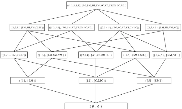
Example 8 Based on Table 1, an object-oriented formal concept lattice can be derived and illustrated in Figure 5. Rectangles represent the object-oriented formal concepts in the lattice. Lines between rectangles express the partial order relations among the concepts. From Figure 4 and Figure 5, one can reveal that a concept in the object-oriented concept lattice can be obtained by taking the set complements of the concept in the property-oriented concept lattice, and vice verse.
Consider the operator23 : 2U →2U, which is an interior operator on 2U [14,18].
The properties of this operator are: forA, A1, A2 ⊆U.
(LI) ∅23=∅,
(LII) A⊆A23,
(LIII) A23 =A2323,
(LIV) A1 ⊆A2 =⇒A231 ⊆A232 .
The properties (LI) and (LII) state that the empty set ∅ will not be changed
under the operator 23. The properties (LIII) - (LIV) mean that 23 is an
idempotent and monotonically decreasing operator.
Let (U,23) denote the family of sets (U,23) = {A23 | A ⊆ U}. It contains
( {1 ,2 ,3 ,4 ,5 }, {P O ,L M ,SM ,VM ,VC ,A T ,C S,D M ,I C ,A D })
( {1 ,2 ,5 }, {L M ,SM ,VM ,C S,I C }) ( {1 ,2 ,3 ,4 }, {P O ,L M ,A T ,C S,D M ,I C ,A D }) ( {2 ,3 ,4 ,5 }, {SM ,VC ,A T ,C S,D M ,I C }) ( {1 ,3 ,4 ,5 }, {L M ,SM ,VM ,VC })
({1,2}, {LM ,CS,IC}) ({1,5}, {LM ,SM ,VM } ) ({2,3,4}, {A T ,CS,D M ,IC}) ({2,5}, {SM ,CS,IC}) ({3,4,5}, {S M,VC})
({1}, {LM}) ({2}, {CS ,IC}) ({5}, {S M})
(ø ,ø )
Fig. 5. The Lattice of Object-oriented Concepts
object-oriented formal concepts. The properties of the system (U,23) are:
(L1) U ∈(U,23),
(L2) A1, A2 ∈(U,23) =⇒A1∪A2 ∈(U,23).
These properties state that the system (U,23) is closed under the operator23
and the set union∪, but not closed under set intersection ∩.
5.6 Connections between Different Lattices
Based on the connections of modal-style data operators, the concepts in
vari-ous lattices can be expressed by equivalence classes as follows. ForA⊆U, B ⊆
V, A∗∗=[{[x]|x∈U, A∗ ⊆xR}, A##=[{[x]|x∈U, A#∪xR6=V}, A23=[{[x]|x∈U, A2∩xR6=∅}, A32=[{[x]|x∈U, xR⊆A3}, and B∗∗=[{[y]|y∈V, B∗ ⊆Ry},
B##=[{[y]|y∈V, B#∪Ry 6=V}, B23=[{[y]|y∈V, B2∩Ry6=∅},
B32=[{[y]|y∈V, Ry ⊆B3}.
It follows that different types of lattices can be connected and transformed from each other by using equivalence classes. The equivalence classes can be considered as a base to construct different types of lattices.
6 Conclusion
In this paper, we propose an approach to investigate multiple views of intelli-gent data analysis based on modal-style data operators. We provides a basic framework to explore the significant importance of multiview for the research on intelligent data analysis. The integration of these multiple views may bring more powerful and useful data analysis tools.
By defining various types of data operators, we present various data relation-ships and construct different types of hierarchical structures, which provides different granulated views of the data. A type of data relationships has a spe-cific semantic interpretation and may be considered as a type of knowledge discovered from a data set. Different types of data relationships present dif-ferent types of knowledge. Difdif-ferent hierarchical structures defined based on modal-style data operators represent various aspects or features of data and can be viewed as multiple types of knowledge embedded in the data.
For future work, we will study the connections and transformations between different data relationships or data structures. A general framework to study different views and their connections and transformations may bring more insights into intelligent data analysis.
References
[1] Agrawal, R., Imielinski, T., and Swami, A. Mining association rules between sets of items in large databases, Proceedings of International Conference on Mangement of Data (ACM SIGMOD), 207-216, 1993.
[2] Aleksander, I. and Morton, H.An Introduction to Neural Computing, Chapman & Hall, London, 1990.
[3] Amari, S. Mathematical foundations of neurocomputing, Proceedings of the IEEE,78, 1443-1463, 1990.
[4] Anderberg, M.R.Cluster Analysis for Application, Academic Press, New York, 1973.
[5] Bajcsy, R. and Kovacic, S. Multiresolution elastic matching, Computer Vision Graphic Image Processing,46, 1-21, 1989.
[6] Bargiela, A. and Pedrycz, W. Granular Computing: an Introduction, Kluwer Academic Publishers, Boston, 2002.
[7] Belkhouche, B. and Lemus-Olalde, C. Multiple veiw analysis of designs,
Foundations of Software Engineering, Joint proceedings of the 2nd International Software Architecture Workshop (ISAW-2) and International Workshop on Multiple Perspectives in Software Development, (SIGSOFT’96), 159-161, 1996. [8] Belkhouche, B. and Lemus-Olalde, C. Multiple views analysis of softweare designs, International Journal of Software Engineering and Knowledge Engineering,10, 557-579, 2000.
[9] Breiman, L., Friedman, J.H., Olshen, R.A. and Stone, C.J. Classification and Reggression Trees, Wadsworth, Califoria, 1984.
[10] Buszkowski, W. Approximation spaces and definability for incomplete information systems,Rough Sets and Current Trends in Computing, Proceedings of the 1st International Conference (RSCTC’98), 115-122, 1998.
[11] Chen, Y.H. and Yao, Y.Y. Multiview Intelligent Data Analysis based on Granular Computing, Proceedings of 2006 IEEE International Conference on Granular Computing (Grc’06), 281-286, 2006.
[12] Cohn, P.M.Universal Algebra, Harper and Row Publishers, New York, 1965. [13] Cover, T.M. and Hart, P.E. Nearest neighbor pattern classification, IEEE
Transactions on Information Theory,IT-13, 21-27, 1967.
[14] D¨untsch, I. and Gediga, G. Approximation operators in qualitative data analysis, in: Theory and Application of Relational Structures as Knowledge Instruments, de Swart, H., Orlowska, E., Schmidt, G. and Roubens, M. (Eds.), Springer, Heidelberg, 216-233, 2003.
[15] Ester, M., Kriegel, H.P., Sander, J., and Xu, X. A density-based algorithm for discovering clusters in large spatial data sets with noise.Proceedings of the 2nd International Conference on Knowledge Discovery and Data Mining. 226-231, 1996.
[16] Freitas, A.A. Understanding the crucial differences between classification and discovery of association rules - A position paper, SIGKDD Explorations, 2, 65-69, 2000.
[17] Ganter, B. and Wille, R.Formal Concept Analysis: Mathematical Foundations, Springer-Verlag, New York, 1999.
[18] Gediga, G. and D¨untsch, I. Modal-style operators in qualitative data analysis,
Proceedings of the 2002 IEEE International Conference on Data Mining, 155-162, 2002.