Solving Mixed-Integer Quadratic Programs
via Nonnegative Least Squares
Alberto Bemporad⇤
⇤IMT Institute for Advanced Studies Lucca, Italy
(email: [email protected]).
Abstract:This paper proposes a new algorithm for solving Mixed-Integer Quadratic Program-ming (MIQP) problems. The algorithm is particularly tailored to solving small-scale MIQPs such as those that arise in embedded hybrid Model Predictive Control (MPC) applications. The approach combines branch and bound (B&B) with nonnegative least squares (NNLS), that are used to solve Quadratic Programming (QP) relaxations. The QP algorithm extends a method recently proposed by the author for solving strictly convex QP’s, by (i) handling equality and bilateral inequality constraints, (ii) warm starting, and (iii) exploiting easy-to-compute lower bounds on the optimal cost to reduce the number of QP iterations required to solve the relaxed problems. The proposed MIQP algorithm has a speed of execution that is comparable to state-of-the-art commercial MIQP solvers and is relatively simple to code, as it requires only basic arithmetic operations to solve least-square problems.
Keywords:Mixed-integer quadratic programming, Quadratic Programming, Active set methods, Nonnegative least squares, Model predictive control, Hybrid systems.
1. INTRODUCTION
After the first paper (Bemporad and Morari, 1999), hybrid Model Predictive Control (MPC) has received tremendous attention, both by academic researchers and industrial engineers. The main reason is the large variety of complex control problems that the approach can handle, due to the ability of capturing in the same model multiple linear dynamics, logic variables and states, mixed linear and logical constraints, meeting closed-loop performance and constraint satisfaction requirements in a rather direct, ef-fective, and systematic way (Bemporad and Morari, 1999). As for linear and nonlinear MPC, this success would not have been possible if good numerical solvers were not available to solve Mixed-Integer Quadratic Programming (MIQP) or mixed-integer linear programming problems, and to automatize the translation of the hybrid control problem into a computationally-tractable form (Torrisi and Bemporad, 2004). In fact, evaluating the hybrid MPC control decision on line requires solving an MIQP at each time step. While to date very efficient commercial solvers exist to solve MIQPs (Gurobi Optimization, Inc., 2014; IBM, Inc., 2014; Fair Isaac Corporation, 2015), these are not tailored to embedded applications on low-cost/low-power control boards. E↵orts in this direction were re-cently proposed by Frick et al. (2015), extending an em-bedded convex programming solver based on interior-point methods to a Branch and Bound (B&B) setting (Floudas, 1995). Another approach for B&B-based MIQP tailored to MPC problems was proposed by Axehill and Hansson (2006), where a dual QP method is employed and warm-started from parent-node solutions, and optimality
condi-? This work was partially supported by the H2020 European
project DISIRE, Grant Agreement No. 636834,http://spire2030. eu/disire/.
tions are solved using Riccati recursions. The method does not exploit however dual lower bounds on the optimal cost, that is instead particularly useful to reduce the number of solved QP relaxations (Fletcher and Ley↵er, 1998). In this paper, we propose a B&B method to solve MIQPs that leverages on a novel solution algorithm for strictly convex QPs recently developed by the author (Bemporad, 2015b). Such a QP solver is an active set method based on a nonnegative least squares (NNLS) reformulation of the quadratic optimization problem, is quite fast and simple to code, and, contrary to iterative methods, converges after a finite number of iterations to the solution, rather insensitively with respect to preconditioning of problem matrices. The advantage of the method is that it relies on solving least-squares problems, probably one of the most studied problems in numerical linear algebra, so that an abundance of fast and robust numerical techniques are available for its implementation. The benefits of using non-negative least squares in MPC was recently investigated by the author, both for embedded linear MPC based on QP (Bemporad, 2015b) and for solving the multiparamet-ric quadratic programming (mpQP) problems that arise in explicit MPC (Bemporad, 2015a).
To be able to use the QP solver of (Bemporad, 2015b) as the core engine for solving QP relaxations during branching, this paper first extends the algorithm to the case of equality and bilateral inequality constraints, to warm starting from previous solutions, and to compute dual lower bounds on the optimal cost.
We show in examples that the resulting MIQP solver is quite competitive with respect to commercial packages, at least to solve small-scale MIQPs that arise in typical
embedded hybrid Model Predictive Control (MPC) appli-cations.
1.1 Notation
Let Rn denote the set of real vectors of dimension nand N the set of natural integers, respectively, and let I ⇢N be a finite set of integers. For a vectora2Rn, ai denotes thei-th entry ofa,aIthe subvector obtained by collecting the entriesai for alli2I,kak2 the Euclidean norm ofa,
kak1 =Pni=1|ai| the 1-norm ofa, the conditiona >0 is
equivalent to ai >0, 8i = 1, . . . , n (and similarly for ,
, <), and diag(a) is the diagonal matrix whose (i, i)-th element is ai. We denote by 0n the vector of Rn with all zero components, with the subscript n dropped whenever the dimension is clear from the context. For a matrix A 2 Rn⇥m, A0 denotes its transpose, Ai denotes the i
-th row ofA,AI the submatrix ofAobtained by collecting the rows Ai for all i 2 I, and AIJ the submatrix of A
obtained by collecting the rows and columns ofAindexed by i 2 I and j 2 J, respectively. Matrix A# 2 Rm⇥n denotes the pseudoinverse matrix of A, namelyAA#A=
A, A#AA#=A#,AA#= (AA#)0,A#A= (A#A)0 (ifA
is full column rank,A#,(A0A) 1A0). For a square matrix A 2 Rn⇥n, A 1 denotes the inverse of A (if it exists)
and A T its transpose, A 0 (A
⌫0) denotes positive definiteness (semidefiniteness) ofA. MatrixIn denotes the identity matrix of ordern, where sometimes the subscript nis dropped if the dimension is clear from the context.
2. PROBLEM FORMULATION
We want to solve the following class of Mixed-Integer Quadratic Programming (MIQP) problems
min z V(z), 1 2z 0Qz+c0z (1a) s.t. `Azu (1b) Gz=g (1c) ¯ Aiz2{`¯i,ui¯ }, i= 1, . . . , q (1d) where Q 0 is the Hessian matrix, Q2 Rn⇥n, c
2Rn, A 2 Rm⇥n, `, u 2 Rm, ` u, G 2 Rp⇥n, g 2 Rp, ¯ A 2 Rq⇥n, ¯`,u¯ 2 Rq. Binary constraints zi 2 {0,1} are a special case of (1d), obtained by setting ¯Ai as thei-th row of the identity matrix, ¯`i= 0, and ¯ui= 1.
MIQP problems of the form (1) arise when formulating hybrid MPC controllers based on the following Mixed Logical Dynamical (MLD)
xk+1 =Axk+B1vk+B2 k+B3⇣k+B5 (2a)
yk =Cxk+D1vk+D2 k+D3⇣k+D5 (2b)
E2 k+E3⇣kE1vk+E4xk+E5, (2c)
model representation, wherexkis the state vector,ykis the output vector,vk is the input vector,⇣k and k are auxil-iary vectors. Vector⇣kis real-valued, kis binary,xk, uk, yk can contain both real and binary components. MatricesA,
Bi, C, Di and Ei are constant and determine the hybrid dynamics. They can be obtained automatically by high-level descriptions of the hybrid dynamics and constraints, for example by using the translation tool HYSDEL (Torrisi and Bemporad, 2004). The MLD model (2) is used to formulate the following hybrid MPC problem
min {vk,k,⇣k}Tk=01 TX1 k=0 kLx(xk rxk)k22+kLv(vk rvk)k22+ (3a) kL⇣(⇣k r⇣k)k 2 2+kL ( k rk)k22 s.t. MLD model (2) (3b) x0=x(t)
that can be mapped into a MIQP problem of the form (1), with z = [v00 ... vN0 1 00 ... N0 1 ⇣00...⇣N0 1]0 2 Rn, ¯` = 0,
¯
u= 1, and ¯A containing the rows of the identity matrix In corresponding to the binary components of vector z. We have assumed that matrixQin (1a) is positive definite. In many hybrid MPC formulations this is not the case, as some of the weight matrices Lx, Lv, L⇣, L may not be
full-rank and lead to a resulting Hessian matrixQ⌫0. In such cases, we assume the problem gets modified by adding a regularization term⇢IntoQ, 0<⇢⌧1. We will show in Section 5.2 that this does not change the computed hybrid MPC action significantly.
3. EXTENDED QP SOLVER BASED ON NNLS The core ingredient of the MIQP algorithm proposed in this paper is the QP solver developed in (Bemporad, 2015b) for minimizing strictly convex quadratic functions subject to inequality constraints. Such a QP solver is based on the idea of rephrasing a strictly convex QP problem as a Least Distance Problem (LDP) that is solved via a NNLS algorithm, and was shown very efficient in (Bempo-rad, 2015b) compared to existing state-of-the-art QP algo-rithms. In this section we extend the algorithm to handle bilateral inequalities (1b), equality constraints (1c), warm starting, and early stopping, so that it can be efficiently exploited within a branch & bound (B&B) framework. The resulting extended method to solve the QP problem (1a)– (1c) is described in Algorithm 1.
We justify the various steps of Algorithm 1 in the following sections.
3.1 Bilateral inequalities and equalities
The dual QP problem of (1a)–(1c) is the following convex QP max `, u,µ ( `, u, µ), 1 2 h ` u µ i0h A A G i Q 1· [ A0 A0G0] h ` u µ i d` du f 0h ` u µ i 1 2c 0Q 1c (8a) s.t. `, u 0, µfree, (8b)
where `, u 2Rm,µ2Rp, andd`, du 2Rm, f 2Rp are
defined as follows:
d`, ` AQ 1c, du,u+AQ 1c, f ,g+GQ 1c. (8c)
The following theorem shows how the QP problem (1a)– (1c) is equivalent to a least squares problem in which some of the variables are constrained to be nonnegative, extending (Bemporad, 2015b, Th. 1) to the case of equality and bilateral inequality constraints.
Theorem 1. Consider the QP (1a)–(1c) and let Q 0. Let L0L be a Cholesky factorization of Q and define
Algorithm 1 QP solver based on NNLS with equality constraints, bilateral inequalities, warm start, and early stop
Input: Inverse Cholesky factorL 1 ofQ; matricesM =
AL 1,N =GL 1; vectorsc,v=L Tc,d`= (`+M v), du=u+M v,f =g+N L Tc; initial guess
Pu,P`, vectors y`, yu, w`, wu,⌫, a, scalar , ,V satisfying (13), (14), (15);
max tolerable value V0 for the optimal cost; feasibility
tolerance✏ 0. 1. k 0; 2. if (min{w`, wu} ✏ orP`[Pu ={1, . . . , m} or a0a+ 2 = 0 or V > V 0) and k > 0 then go to Step 8; 3. k k+ 1;i` arg mini2{1,...,m}\P`w`i, iu arg mini2{1,...,m}\Puwui;
4. if w`i` wuiu thenP` P`[{i`}; +|d`i`|; otherwisePu Pu[{iu}; +|duiu|; 5. s`, su 0m;
6. solvethe least squares (LS) problem
hs`P` suPu s⌫ i arg min z MP0` MP0u N0 d0 `P` d 0 uPu f0 z+⇥0n⇤ 2 2 ; (4) 7. if s`P`, suPu 0then hy` yu ⌫ i hs` su s⌫ i ; a M0(yu y`) +N0⌫; (5a) +d0`y`+d0uyu+f0⌫; (5b) [w` wu] M a ⇥ I I ⇤ + ⇥d` du ⇤ ; (5c) V as in (14b); (5d) go toStep 2; otherwise ↵` min h2P`:s`h0 ⇢ y `h y`h s`h ; ↵u min h2Pu:suh0 ⇢ yuh yuh suh ; hy` yu ⌫ i hy` yu ⌫ i +⇣hssu` s⌫ i hy` yu ⌫ i⌘ ·min{↵`,↵u}; I` {h2P`:y`h= 0},P` P`\ I`; kd`I`k1; Iu {h2Pu:yuh= 0};Pu Pu\ Iu; kduIuk1; go toStep 5;
8. if the residual in Step 6 is nonzero then if V V0 then z⇤ L 1 ✓ 1 a+v ◆ ; ⇤ ` ⇤ u µ⇤ 1hy` yu ⌫ i ; (7a) V⇤ V; (7b) otherwiseV⇤> V 0;
otherwiseQP problem is infeasible; 9. end.
Output: Primal solution z⇤ of the QP problem (1a)– (1c); optimal Lagrange multipliers ⇤
`, ⇤u 0 of lower and upper bound constraints (1b) and µ⇤ of equality constraints (1c); optimal cost V⇤, or infeasibility status,
or proof thatV⇤> V
0; numberkof iterations.
M ,AL 1,N,GL 1. Let be any positive scalar.
Con-sider the Partially Nonnegative Least Squares (PNNLS) problem min y 1 2 M0 d0` y` M0 d0u yu N0 f0 ⌫ 0 2 2 (9a) s.t. y`, yu 0, ⌫ free (9b)
withy`, yu2Rm,⌫ 2Rp, and let r⇤,
M0(y`⇤ yu⇤) N0⌫⇤
d0`y⇤` d0uyu⇤ f0⌫⇤ , (10) be the residual obtained at the optimal solution (y`⇤, y⇤u,⌫⇤) of (9), wherey⇤
`, y⇤u 2Rm, ⌫⇤ 2Rp, andr⇤ 2 Rn+1. The following statements hold:
i) Ifr⇤= 0 then QP (1a)–(1c) is infeasible; ii) Ifr⇤6= 0 then z⇤, Q 1 ✓ c+ A0(yu⇤ y⇤`) +G0⌫⇤ +d0 `y`⇤+d0uy⇤u+f0⌫⇤ ◆ (11) solves QP (1a)–(1c).
Proof.See Appendix A. 3.2 Properties of the solution
The following Lemma 1 shows the properties of the primal and dual solutions that one could reconstruct during the iterations of Algorithm 1 as in (7a) below, as well as the corresponding primal and dual objective functions. Lemma 1. Lety`, yu,⌫,aand be defined as in (5a)–(5b)
for a given > 0, with s`, su 0 and s⌫ obtained by
solving the LS problem (4), and let >0. The primal cost associated with z = L 1 1a+v , v = L Tc, and the dual cost associated with vectors `= 1y`, u= 1yu, and µ= 1⌫ are such that
( `, u, µ) = 1 2 a0a 2 1 2v 0v (12a) V(z) =1 2 ✓ a0a 2 v0v ◆ (12b) ( `, u, µ) =V(z)V(z⇤). (12c)
Proof. Since > 0 and y` = s` 0, yu = su 0, we
have that the triplet ( `, u, µ) is feasible for the dual QP
problem (8), and therefore the inequality ( `, u, µ) V(z⇤) in (12c) is satisfied. Equality (12a) follows by (5a)–
(5b) and substituting `, u, µ in the dual cost (8a). By
substituting the expression for z in (1a) we obtain the second equality (12b). Equality (12c) follows from (5) and from the conditions of optimality of (9) related to complimentary slackness, that is y0
`w`+yu0wu = 0, and of ⌫ as a function of y`, yu given by (Bemporad, 2015a,
Lemma 1), that is (N N0 +f f0)⌫ N M0y
` +N M yu+ f d0`y`+f d0uyu⇤+ f = 0 (cf. the proof of Theorem 1 in Appendix A).
In case > 0, by (12c) of Lemma 1 the quantity z as in (7a) is always super-optimal during the iterations of Algorithm 1 (and, if it is strictly super-optimal, is also necessarily infeasible); it only becomes optimal (and therefore feasible) when the algorithm terminates with a nonzero residual.
3.3 Warm starting
We consider as a valid warm start the initial active sets
Pu,P` ✓{1, . . . , m}, initial guessy`, yu, w`, wu 2Rmand
⌫ 2Rpfor the PNNLS problem (9) satisfying the following conditions: Pu\P`=; (13a) y`, yu 0, (13b) ⌫= hN0 f0 i#h M0(yu y`) i (13c) w`= M M0(yu y`) + d` (13d) wu=M M0(yu y`) + du (13e) y`0w`=yu0wu= 0 (13f) y`i 0, w`i= 0, 8i2P`, (13g) yui 0, wui= 0, 8i2Pu (13h) y`i= 0, 8i2{1, . . . , m} \ P` (13i) yui= 0, 8i2{1, . . . , m} \ Pu, (13j) where =d0`y`+d0uyu+ (13k) along with the following quantities
a=M0(yu y`) +N0⌫ (14a) V =1 2 ✓a0a 2 v0v ◆ . (14b)
See the proof of Theorem 1 for a justification of condi-tions (13) and of Lemma 1 for condicondi-tions (14).
3.4 Early stopping criteria
By exploiting the result of Lemma 1, Algorithm 1 has been formulated for solving the QP problem (1a)–(1c) only if the optimal solutionV(z⇤)V
0, whereV0is a given value
(possibly V0 = +1). This is of particular importance, in
that it allows to halt immediately Algorithm 1 at Step 2 after computing (5) at Step 7, in case the quantity V in (14b) is greater thanV0. This feature will be particularly
useful in the B&B setting described in next Section 4. The following Corollary 1 of Theorem 1 (that extends (Be-mporad, 2015b, Corollary 2) to the equality constrained case) justifies the stopping condition a0a + 2 = 0 at
Step 2, providing a simple yet very e↵ective criterion to early detecting the infeasibility of the QP problem (1a)– (1c). In the numerical implementation of Algorithm 1, the condition a0a+ 2 = 0 is replaced by a0a+ 2
✏infeas, where✏infeas>0 is a small tolerance.
Corollary 1. Lets`, sua solution of problem (4), lets`, su,
and let a, be defined as in (5). Ifa0a+ 2= 0 then the
QP problem (1a)–(1c) is infeasible.
Proof. The quantity a0a+ 2 is equal to the residual of
problem (4). As proved in part i) of Theorem 1, if such a residual is zero then the polyhedron C , {u 2 Rn : MPuuu, MP`u `, N u=f} is empty. Hence, also the polyhedron {u2Rn : M uu, M u `, N u=f} =C\ {u2 Rn : M
{1,...,m}\Puu u, M{1,...,m}\P`u `, N u = f}is empty, and therefore problem (1a)–(1c) is infeasible.
3.5 Improving numerical robustness
The basic NNLS algorithm of Lawson and Hanson (1974) is formulated for = 1. As suggested in (Bemporad, 2015b), we choose here to adapt during iterations to the following value
= 1 +kfk1+kd`P`k1+kduPuk1 (15) which provides better numerical conditioning.
Although less critical than with iterative methods like accelerated gradient projection (Patrinos and Bemporad, 2014) and ADMM (Boyd et al., 2011), preconditioning the MIQP problem (1) sometimes ensures a better numerical robustness of Algorithm 1. However, contrary to iterative methods, in active set methods the e↵ect of scaling the variables of the problem is much less critical, as the total number of iterations may decrease, remain constant, or even increase sometimes. In case preconditioning is needed, we suggest here to use Jacobi diagonal scaling of the inequality constraints (1b) defined as follows (Bertsekas, 2009): ✓i, 1 kMik2 (16a) M diag(✓1, . . . ,✓m)M (16b) `i ✓i`i (16c) ui ✓iui, i= 1, . . . , m. (16d)
4. MIQP SOLVER BASED ON NNLS
The B&B Algorithm 2 solves the convex MIQP prob-lem (1) by exploiting the features o↵ered by Algorithm 1. The setsQ`,Qu initialized at Step 2 represent the sets of indices corresponding to the equality constraints induced by setting, respectively, ¯Aiz = ¯`i or ¯Aiz = ¯ui during branching. The tuple A collects the input arguments to Algorithm 1, while S is an ordered list of tuples, corre-sponding to the equality-constrained QP’s that remain to be solved. At Step 3.1 the last element A of S is extracted to solve the corresponding MIQP relaxation, corresponding to a depth-first search.
After executing Algorithm 1 at Step 3.2, the final values ofP`,Pu, M, y`, yu, w`, wu,⌫, d`, du, , , a, V⇤are kept and
used (if needed) to warm start the subsequent QP relax-ations. Note that in this caseV⇤ becomes a lower bound
for all children QP problems, as these include additional equality constraints. Step 3.3.1 is only executed if the QP relaxation was feasible and did not halt because the conditionV > V0 was satisfied (that is, the relaxation was
proven to a worse cost than the cost of the best integer-feasible solution found so far). In this case, Step 3.3.1 checks whether all integrality constraints are satisfied, where the quantity ti , 1Mi¯ (a L Tc) = ¯Aiz⇤, and
eventually updates the best known integer-feasible solu-tion⇣⇤ and its corresponding costV
0. Otherwise,
branch-ing is executed at Steps 3.3.3.1–3.3.3.8 by pickbranch-ing up the indexib corresponding to the constraint ¯Aiz that is most distant from ¯`i,ui¯ (Step 3.3.3.1). Such a constraint is moved from the set of inequality constraints to the set of equality constraints at Step 3.3.3.2, and two new MIQP relaxationsA0,A1are formed at Step 3.3.3.7.
To prove that the warm-starting vectors in A0, A1
sat-isfy (13)–(15), note that y`, yu,⌫ are generated at Step 7
of Algorithm 1 after solving the LS problem (4). Hence, (y`, yu,⌫0) and (y`, yu,⌫1) satisfy (13c). In addition,y`,yu, w`, wu are an output of Algorithm 1, so they satisfy the
conditions of QP optimality, and in particular (13b), that remains satisfied after executing Step 3.3.3.4, and (13d)– (13i). Clearly, the warm-start combination of vectors may not be optimal, due to forcing the equality constraint
¯
Aibz = ¯`i (or ¯Aibz = ¯ui) in the active set of the new relaxed QP problem.
Step 3.3.3.8 chooses to solve first the MIQP relaxation corresponding to the quantity tib that is closest to the lower value`ibor upper valueuib. When no relaxations are left to solve, Step 4 checks whether the initial upper-bound V0 has remained +1, in which case no integer feasible
solution was found.
4.1 Double-inequality formulation
In Steps 3.3.3.2–3.3.3.3, Algorithm 2 fixes binary con-straints (1d) as either the equality constraint ¯Aiz = ¯`i or ¯Aiz = ¯ui. An alternative approach to equivalently fix
¯
Aiz = ¯`i is to transform the relaxed inequality ¯Aiz ui¯ into the inequality Aiz¯ `¯i (and, similarly ¯Aiz `¯i into ¯Aiz ui¯ to fix ¯Aiz = ¯ui). To change the lower bound from ¯`i to ¯ui one simply subtracts the quantity ¯
`i ui¯ from d`i (and, similarly ¯ui `¯i from dui) before creating the children relaxed QP problems at Step 3.3.3.7. In this way, matrices Nb ⌘ N0, Mb ⌘ M, f0 = f1 ⌘ f
remain constant during the execution of the algorithm, as it is enough to update only vectors d`i, dui. While the approach is appealing for its simplicity, it may lead to a possible increased number of iterations when solving the QP relaxation via Algorithm 1. Moreover, the unavoidable introduction of a tolerance " when imposing the upper bound ¯Aiz`¯i+"(and, similarly, ¯Aiz ui¯ ") must be taken care of accurately to avoid numerical issues.
5. NUMERICAL RESULTS
In this section we report numerical experiments obtained on a Macbook Pro 3GHz Intel Core i7 with 16GB RAM running MATLAB R2014b.
5.1 Random mixed-integer quadratic programs
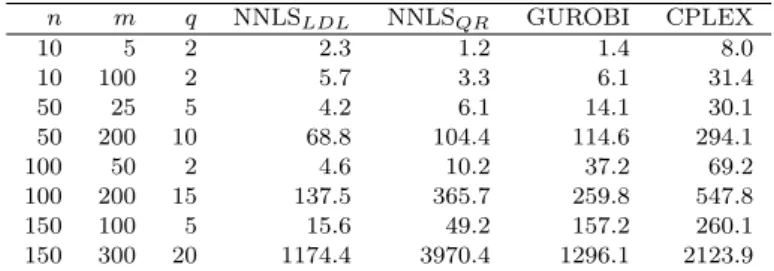
We compare the performance of the MIQP solver de-veloped in the previous sections (labeled as NNLS) against the commercial state-of-the-art MIQP solver of GUROBI v6.0 (Gurobi Optimization, Inc., 2014) and of CPLEX (IBM, Inc., 2014) with default options. Presolvers were disabled for fairness of comparison, although they do not contribute significantly to change computation time (sometimes even worsen it). Algorithm 1 has been implemented in Embedded MATLAB code and compiled, Algorithm 2 is run in interpreted MATLAB code.
Table 1 shows the CPU time obtained for solving feasible MIQP problems with n variables, m bilateral linear in-equality constraints,pbinary constraints of the formzi 2 {0,1}, and condition number= 104of the primal Hessian
Algorithm 2MIQP solver based on NNLS
Input: MIQP problem matrices Q =Q0 0, A, G, ¯A
and vectors`,u,g, ¯`, ¯u; feasibility tolerance✏ 0. 1. Compute inverse Cholesky factorization Q 1 =
L 1L T; v L Tc; 2. set M0 ⇥AA¯⇤L 1, d` = ⇥``¯⇤ M0L Tc, du = [u¯ u] +M0L Tc; N0 GL 1,f g+N0L Tc; P`,Pu ;,y`, yu, w`, wu 0q+m; , 1 +kfk1, ⌫ (N0N00+f f0) 1f ; a M0(yu y `) +N0⌫; V 12⇣a02a v0v ⌘ ;V0 +1; ⇣⇤ ;;Q `,Qu ;;
A {P`,Pu, M0, N0, f, y`, yu, w`, wu,⌫, d`, du, , , a, V,Q`,Qu};
S {A}; 3. while S6=;do:
3.1. getlast elementA2S;setS S \ {A}; 3.2. executeAlgorithm 1 with input fromAandget
z⇤, V⇤,P
`,Pu, y`, yu, w`, wu,⌫, d`, du, , , a;
3.3. if QP problem feasibleand V⇤V0 then
3.3.1. if (Q`[Qu={1, . . . , q}orti, 1Mi¯ (a L Tc) 2{`i, ui},8i= 1, . . . , q) thenV0 V⇤, ⇣⇤ z⇤;otherwise 3.3.3.1. ib arg min i2{1,...,q}\(Q`[Qu) ti `i+ui 2 ; 3.3.3.2. J Q`[Qu[{ib};I {1, . . . , q}\J; 3.3.3.3. Nb hM¯N J i ;Mb ⇥M¯I M ⇤ ;
3.3.3.4. y` vector of components of y` after
eliminating the component y`b corre-sponding toib (same foryu, w`, wu);
3.3.3.5. f0 2 4 f ¯ `Q` ¯ uQu ¯ `ib 3 5+NbL Tc; f1 " f ¯ `Q` ¯ uQu ¯ uib # +NbL Tc; 3.3.3.6. ⌫0 [y⌫`b];⌫1 [ ⌫ yub]; 3.3.3.7. A0 {P`,Pu, Mb, Nb, f0, y`, yu, w`, wu, ⌫0, d`, du, , , a, V⇤,Q`[{ib},Qu}; A1 {P`,Pu, Mb, Nb, f1, y`, yu, w`, wu, ⌫1, d`, du, , , a, V⇤,Q`,Qu[{ib}}; 3.3.3.8. if tib `i+ui 2 thenS S[{A1,A0}; otherwiseS S[{A0,A1};
4. if V0 = +1then(1) is infeasible otherwiseV⇤
V0;
5. end.
Output: Solution⇣⇤ of the MIQP problem (1), optimal
costV⇤, or infeasibility status.
Q1. The reported time is the worst-case obtained over 20
instances for each triplet n, m, p. Problem (4) in Algo-rithm 1 is solved by updating the LDLT decomposition
1 The entries of matrixAare generated from the normal distribution
N(0,0.0025), `, u from the uniform distribution U(0,1), c from N(0,100); matrixQ=U⌃V0, whereU, V are orthogonal matrices generated by QR decomposition of randomn⇥nmatrices, and⌃ is diagonal with nonzero entries having logarithms equally spaced between±log()/4 (Bierlaire et al., 1991).
(NNLSLDL in the table) of MP ` d`P` MPu duPu N f MP0` MP0u N0 d0`P` d 0 uPu f 0 recursively as described in (Bemporad, 2015b) when the dimension of vectorhyyu`
⌫
i
is smaller or equal thann, and, for improved numerical robustness, QR factorization in case more than n elements must be optimized in Prob-lem (4). As an alternative, we purely updated the QR factorization of the same matrix (NNLSQR in the table) recursively as described in (Lawson and Hanson, 1974, Chap. 24, Method 1). n m q NNLSLDL NNLSQR GUROBI CPLEX 10 5 2 2.3 1.2 1.4 8.0 10 100 2 5.7 3.3 6.1 31.4 50 25 5 4.2 6.1 14.1 30.1 50 200 10 68.8 104.4 114.6 294.1 100 50 2 4.6 10.2 37.2 69.2 100 200 15 137.5 365.7 259.8 547.8 150 100 5 15.6 49.2 157.2 260.1 150 300 20 1174.4 3970.4 1296.1 2123.9 Table 1. Worst-case CPU time (ms) on random MIQP problems over 20 instances for each
combination of n,m,q.
It is apparent that on such a set of random MIQP problems, Algorithm 2 performs comparably well with respect to the commercial solvers GUROBI and CPLEX, especially when the numberqof binary constraints is small compared to n and m, probably due to the pure B&B nature of Algorithm 2.
The results shown in Table 2 are obtained, under the same conditions, on purely binary quadratic programs (n =q, m= 5n). When turning the presolver on, in GUROBI and CPLEX the results remain rather similar.
n m q NNLSLDL NNLSQR GUROBI CPLEX 2 10 2 5.1 4.0 0.7 8.4 4 20 4 8.9 4.3 4.5 16.7 8 40 8 19.2 18.0 37.1 14.7 12 60 12 59.7 57.8 82.3 47.9 20 100 20 483.5 457.7 566.8 99.6 25 250 25 110.4 93.3 1054.4 169.4 30 150 30 1645.4 1415.8 2156.2 184.5 Table 2. Worst-case CPU time (ms) for random binary QP problems with nvariables and 5m constraints, over 20 instances for each value of
nand the correspondingm,q.
5.2 Hybrid MPC problem
In order to test Algorithm 2 in a hybrid MPC problem (2)– (3), we consider the hybrid control problem described in (Bemporad and Morari, 1999, Example 5.1) with all zero weights except a unit weight on the output of the system (these are the settings of the demo bm99sim.min the Hybrid Toolbox for MATLAB (Bemporad, 2003)) and a prediction horizonT between 2 and 10.
The regularization term 10 4Iwas added on the resulting
Hessian matrix Qto make the resulting MIQP’s positive definite. This induces a small di↵erence in the input and
N NNLSLDL NNLSQR GUROBI CPLEX 2 2.2 2.3 1.2 3.0 3 3.4 3.9 2.0 6.5 4 5.0 6.5 2.6 8.1 5 7.6 9.8 3.7 9.0 6 12.3 17.7 4.3 11.0 7 20.5 30.5 5.8 13.1 8 28.9 47.1 7.3 17.3 9 38.8 62.5 9.5 18.9 10 55.4 98.2 10.9 22.4
Table 3. Hybrid MPC problem: CPU time (ms) per sampling step for di↵erent prediction
horizonsN
output trajectories, however the norm of the di↵erence between the entire trajectories smaller than 0.001. We compare Algorithm 2 with preconditioning (16) against GUROBI and CPLEX with presolvers enabled. The results are reported in Table 3. For T = 10, the MIQP problem has n = 40, q = 10 (i.e., 30 continuous variables and 10 binary variables) and m = 160 linear inequalities. We observed that disabling presolvers in GUROBI and CPLEX sometimes speeds up sometimes slows down the solver.
6. CONCLUSIONS
In this paper we have proposed a new MIQP solver based on B&B that is tailored to embedded hybrid MPC appli-cations. The approach extends an active set method re-cently developed by the author to solve QP relaxations as nonnegative least-squares problems. While the presented approach was shown e↵ective in simulations compared to reference commercial solvers, current research is devoted to combine hybrid models and MIQP solution methods for reaching even higher degrees of e↵ectiveness.
REFERENCES
Axehill, D. and Hansson, A. (2006). A mixed integer dual quadratic programming algorithm tailored for MPC. In Proc. 45th IEEE Conference on Decision and Control, 5693–5698. San Diego, CA, USA.
Bemporad, A. (2003). Hybrid Toolbox – User’s Guide. http://cse.lab.imtlucca.it/~bemporad/ hybrid/toolbox.
Bemporad, A. (2015a). A multiparametric quadratic programming algorithm with polyhedral computations based on nonnegative least squares.IEEE Trans. Auto-matic Control. In press.
Bemporad, A. (2015b). A quadratic programming algo-rithm based on nonnegative least squares with appli-cations to embedded model predictive control. IEEE Trans. Automatic Control. Conditionally accepted for publication.
Bemporad, A. and Morari, M. (1999). Control of systems integrating logic, dynamics, and constraints. Automat-ica, 35(3), 407–427.
Bertsekas, D. (2009). Convex Optimization Theory. Athena Scientific.
Bierlaire, M., Toint, P., and Tuyttens, D. (1991). On iterative algorithms for linear ls problems with bound constraints. Linear Algebra and Its Applications, 143, 111–143.
Boyd, S., Parikh, N., Chu, E., Peleato, B., and Eckstein, J. (2011). Distributed optimization and statistical learning via the alternating direction method of multipliers. Foundations and Trends in Machine Learning, 3(1), 1– 122.
Fair Isaac Corporation (2015). FICO Xpress Optimization Suite. http://www.fico.com/.
Fletcher, R. and Ley↵er, S. (1998). Numerical experience with lower bounds for MIQP branch-and-bound. SIAM J. Optim., 8(2), 604–616.
Floudas, C.A. (1995). Nonlinear and Mixed-Integer Opti-mization. Oxford University Press.
Frick, D., Domahidi, A., and Morari, M. (2015). Embed-ded optimization for mixed logical dynamical systems. Computers & Chemical Engineering, 72, 21–33.
Gurobi Optimization, Inc. (2014). Gurobi Optimizer Ref-erence Manual. URLhttp://www.gurobi.com.
IBM, Inc. (2014).IBM ILOG CPLEX Optimization Studio 12.6 – User Manual.
Lawson, C. and Hanson, R. (1974). Solving least squares problems, volume 161. SIAM.
Patrinos, P. and Bemporad, A. (2014). An accelerated dual gradient-projection algorithm for embedded linear model predictive control. IEEE Trans. Automatic Con-trol, 59(1), 18–33.
Rockafellar, R. (1970). Convex Analysis. Princeton University Press.
Torrisi, F. and Bemporad, A. (2004). HYSDEL — A tool for generating computational hybrid models. IEEE Trans. Contr. Systems Technology, 12(2), 235–249.
APPENDIX A: PROOF OF THEOREM 1 The proof extends the proof reported in (Bemporad, 2015b) to the case of equality bilateral inequality con-straints. First, by defining u ,Lz+L Tc, we complete the squares in (1a) by substitutingz=L 1u Q 1cand
recast (1) into the equivalent constrained Least Distance Problem (LDP) min u 1 2kuk 2 (17a) s.t. Mud (17b) N u=f (17c) whereM,⇥ M M ⇤ ,d,⇥d` du ⇤ .
i) Assume the optimal residual r⇤ = 0 in (10). Let
⌫⇤
+ ,max{⌫⇤,0}, ⌫⇤ ,max{ ⌫⇤,0} be the positive and
negative parts of ⌫⇤, ⌫⇤ = ⌫⇤ + ⌫⇤, ⌫+⇤,⌫⇤ 0. Then, by (10) we get M0y⇤+N0⌫⇤ + N0⌫⇤ = 0 d0y⇤+f0⌫+⇤ f0⌫⇤ = y⇤,⌫+⇤,⌫⇤ 0 (18) where y⇤ ,hy`⇤ y⇤ u i . By Farkas’s Lemma(Rockafellar, 1970, p. 201), for any >0 (18) is equivalent to infeasibility of
Mud N uf N u f
(19) which is obviously equivalent to (17b)–(17c). Therefore the LDP problem (17) does not admit a solution, and consequently (1).
ii) Consider the KKT conditions for problem (9)
⇥Md N f ⇤ h M0y⇤ N0⌫⇤ d0y⇤ f0⌫⇤ i [I 0]w⇤= 0 (20a) (y⇤)0w⇤= 0 (20b) ⌫⇤ free, w⇤ 0, y⇤ 0 (20c) where w⇤ , hw`⇤ w⇤u i
is the optimal dual variable for prob-lem (9). From (20a) we get
[M d]r⇤ w⇤= 0 (21a)
[N f]r⇤= 0 (21b) and hence the condition r⇤ 6= 0, (20a)–(20b) and (21) imply that 0 < (r⇤)0r⇤= (r⇤)0h Md00 i y⇤+ (r⇤)0hN0 f0 i ⌫⇤ r⇤n+1 = (w⇤)0y⇤ rn⇤+1= rn⇤+1, i.e.,r⇤ n+1= d0y⇤ f0⌫⇤ <0. By letting u⇤, 1 r⇤ n+1 r⇤{1,...,n}= M0y⇤+N0⌫⇤ +d0y⇤+f0⌫⇤, (22)
from (20c) and (21a) we obtain
0w⇤= [M d]r⇤= r⇤n+1[M d] 2 4 r⇤ {1,...,n} rn⇤+1 1 3 5
and hence Mu⇤+d 0, or equivalentlyu⇤satisfies (17b).
Moreover, N u⇤ f = N M0y⇤+N0⌫⇤ +d0y⇤+f0⌫⇤ f = 0 i↵0 =NM0y⇤+N N0⌫⇤+ f+f d0y⇤+f f0⌫⇤= (N N0+ f f0)⌫⇤+ (NM0+f d0)y⇤+ f, or equivalently i↵ ⌫⇤= N0 f0 #✓ M0 d0 y⇤+ 0 ◆ . (23)
Since by (Bemporad, 2015a, Lemma 1) condition (23) is always satisfied at optimality of (9), we have proved that u⇤ also satisfies (17c) and therefore is a feasible
candidate to solve (17). It remains to prove that u⇤ is also optimal for (17). To this end, consider the remaining KKT conditions of optimality for problem (17)
u⇤+M0 ⇤+N0µ⇤= 0 (24a) ( ⇤)0(Mu⇤ d) = 0 (24b) ⇤ 0, ⌫⇤ free. (24c) Let ⇤, 1 r⇤ n+1 y⇤, µ⇤, 1 r⇤ n+1 ⌫⇤. (25) By negativity of r⇤
n+1 and nonnegativity of y⇤ we get
⇤ 0. Moreover, by recalling (22), we get u⇤= 1
r⇤ n+1
(M0y⇤+N0⌫⇤) = M0 ⇤ N0⌫⇤
so that also (24a) is satisfied. To prove (24b) we observe that ( ⇤)0(Mu⇤ d) = 1 r⇤ n+1( ⇤)0(Mr⇤ {1,...,n}+dr⇤n+1) = 1 (r⇤ n+1)2(y ⇤)0[M d]r⇤ = 1 (r⇤ n+1)2(y ⇤)0w⇤ = 0 because
of (21a) and (20b). In conclusion, u⇤ is the optimal
solution of problem (17), and hence the vectorz⇤ defined in (11) solves (1a)–(1c).