Adaptive sharing scheme based sub-swarm multi-objective PSO

Adaptive Sharing Scheme Based Sub-Swarm

Multi-objective PSO

Yanxia Sun

(Department of Electrical and Electronic Engineering Science, University of Johannesburg Johannesburg, South Africa

[email protected])

Zenghui Wang

(Department of Electrical and Mining Engineering, University of South Africa, Johannesburg South Africa

[email protected])

Abstract: To improve the optimization performance of multi-objective particle swarm optimization, a new sub-swarm method, where the particles are divided into several sub-swarms, is proposed. To enhance the quality of the Pareto front set, a new adaptive sharing scheme, which depends on the distances from nearest neighbouring individuals, is proposed and applied. In this method, the first sub-swarms particles dynamically search their corresponding areas which are around some points of the Pareto front set in the objective space, and the chosen points of the Pareto front set are determined based on the adaptive sharing scheme. The second sub-swarm particles search the rest objective space, and they are away from the Pareto front set, which can promote the global search ability of the method. Moreover, the core points of the first sub-swarms are dynamically determined by this new adaptive sharing scheme. Some Simulations are used to test the proposed method, and the results show that the proposed method can achieve better optimization performance comparing with some existing methods.

Keywords: Multi-objective PSO, Adaptive sharing Scheme, Sub-swarm, Pareto front set

Categories: F.2.1, G.3, I.1.2.6

1

Introduction

In 1995, Kennedy et al. proposed a new metaheuristic optimization algorithm called Particle Swarm Optimization (PSO) [Kennedy, 95], and PSO is a stochastic optimization technique that simulates the behaviour of a flock of birds or fish. In the original PSO concept, the particles’ velocities are updated based on two important factors: one is the best position (pbest) of each particle; and another is the best position (gbest) among all the particles. Due to the simple updating formulas and good optimization performance, PSO and its variants have been successfully applied to many single objective optimization problems [Ho, 05]. However, in the real-world applications, the optimization problems often involve optimizing several non-commensurable and often competing objectives [Tan, 05]. Although PSO can be

looked as a good optimization algorithm for solving multi-objective optimization problems, the information sharing method, which inherent to PSO methods, has a tendency to degrade the exploration and exploitation performance [Ho, 05].

Multi-objective optimization is different from single-objective (SO) optimization since the multi-objective optimization must obtain a well-distributed and diverse solution set for finding the final tradeoff. Some multi-objective optimization algorithms including the non-dominated sorting genetic algorithm (NSGA-II & NSGA-III) [Deb, 02], [Bhesdadiya, 16], the strength Pareto evolutionary algorithm (SPEA2) [Zitzler, 01] and multi-objective PSO (MOPSO) [Coello coello, 04], [Tian, 2017], [Zhang, 17] have been proposed for multi-objective optimization problems. During optimization process, the solution points or individuals should be distributed as diversely as possible on the discovered trade-offs. Moreover, it is also important that the solution points or individuals are distributed uniformly in order to achieve consistent transition among the solution points when searching for the most suitable solution from the best possible compromise [Khor, 05].

To improve the optimization performance of single objective PSO, some multi-swarm particle swarm optimization (MPSO) methods have been proposed, such as the master-slave model based MPSO [Yu, 08], ladder function form based PSO [Chen, 09], and so on. At the same time, some multi-swarm multi-objective particle swarm optimization (MMPSO) methods have also been proposed to get good optimization performance for multi-objective optimization problems. Some multi-swarm PSOs [Yen, 03], [Leong, 08] adopt the notion of using a heuristical method to choose several swarms with a fixed swarm size throughout the search process. To improve the optimization performance, the swarm size of some multi-swarm PSOs [Cooren, 11] is adaptive based on a certain strategy. However, there is no MMPSO algorithm which uses the Pareto front information to allocate the sub-swarms. In this study the Pareto front information/points are used to allocate the sub-swarms to find whether the optimization performance can be improved.

This paper proposes a new sub-swarm multi-objective particle swarm optimization (SMOPSO) based on Pareto front points and sharing scheme. To balance the exploitation and exploration, the swarm of particles includes two groups of particles. The first group of particles is consisted of several sub-swarms which are searching some areas around some properly chosen points. The second group of particles are searching the area, which is far away from the first group particles and can improve the explore ability of the particles. To make sure the uniformity of the Pareto front sub-swarms, a proper scheme should be used to assess the density of the Pareto front points and choose the cores of the Pareto front sub-swarms. A new adaptive sharing scheme is proposed and it is a new density assessment technique to guarantee the diversity of the points in the set.

The rest of this paper is organized as follows. MOPSO has been briefly described in Section 2. In Section 3, a new adaptive sharing method is proposed to quantify the distribution quality of a population. The SMOPSO algorithm is described in Section 4. Section 5 demonstrates the simulations for testing the new algorithm and the simulation results have been analysed and investigated. And the conclusions are drawn in Section 6.

2

Brief review of multi-objective particle swarm optimization

For single objective optimization algorithms, the optimization process will usually be terminated when one optimal solution is obtained. However, for most of the multi-objective problems, there may be an optimal solution set which includes a number of solutions. Whether one solution is suitable for an optimization problem which depends on several factors such as user’s choice and problem environment, and hence it is necessary to find the entire set of optimal solutions. Many real-world applications involve complex optimization problems with various competing specifications. In general, a multi-objective optimization problem can be formulated as:

MinF x( )( ( ),f x₁ , f_m( ))x , (1) Subject to x,

where  is the decision (variable) space, Rm is the objective space, and

:  m

F R is made of m real-valued objective functions. If  is a closed and connected region in Rn and all the objectives are functions of x, the problem (1) can be called continuous multi-objective optimization problem. In this study, we focus on continuous multi-objective optimization although the proposed method can be easily extended to discrete multi-objective optimization algorithms.

If there is no information about the preference of objectives, the Pareto optimality based ranking scheme is regarded as a good approach to represent the fitness value of each individual for Multi-Objective Optimization (MOO) [Khor, 05]. The solution to an MOO problem can be described by the form of an alternate trade-off which is called Pareto optimal set or Pareto front set. Each objective function fitness of any non-dominated solution in the Pareto optimal set can only be improved by degrading at least one of other objective functions’ fitness [Sun, 11]. The vector F_a dominates another vector F_b, which can be formulated as









Besides the Pareto optimality based ranking scheme, the uniformity among the distributed solution points or individuals is also an important issue in order to ensure consistent transition among the solution points when searching for the most suitable solution from the best possible compromise, an appropriate density assessment method is needed in multi-objective particle swarm optimization to achieve the uniform distribution in the tangential direction to the currently found trade-off surface by giving biased selection probability at the less crowded region. Currently, there are a few density assessment techniques reported along the development of evolutionary techniques for MOO. Among these density assessment techniques, the sharing scheme [Goldberg, 89] may be the earliest assessment which is widely analyzed and used. To enhance the performance of sharing scheme, it is better to let the sharing scheme adapt to the optimization process and an adaptive sharing scheme will be proposed and used in this study.

For more details on MOP, please refer to references [Coello coello, 04], [ Coello coello, 07].

3

Adaptive sharing assessment scheme

Sharing concept was originally proposed by Goldberg [Goldberg 1989] and it is used to improve the population distribution and prevent genetic drift as well as to search for possible multiple peaks in SO optimization. Fonseca and Fleming [Fonseca, 03] latterly applied it in multi-objective optimization problems. Since then, it has received some attention from researchers and it is looked as one of the important operators in multi-objective evolutionary algorithms.

The sharing scheme determines sub-divisions in the objective space by degrading an individual fitness upon the existence of other individuals in its neighborhood defined by a sharing distance. The niche count mi 



sharing function over all members of the population, where the distance d_ij is the distance between the multi-fitness positions of the particles i and j in the objective space, and Nis the number of the members of the population. The sharing function is defined by 1 ( ) 0        _{ }        ij ij share ij share d if d sh d otherwise (2)

where the parameter can be set to 1 in most cases [Goldberg, 89]. The sharing distance parameter _share can determine the neighbourhood size in terms of radius distance [Khor, 05].

The most important factor for the sharing scheme is how to properly set the sharing distance_share , which is usually unknown in the optimization problems. Moreover, it is difficult to get the information of the size of the objective space in advance since it is difficult to determine the exact bounds of the objective space. Fonseca and Fleming [Fonseca, 03] proposed the Kernel density estimation method to determine an appropriate sharing distance for MOO. However, this sharing process is performed in the ‘sphere’ space which may not properly reflect the Pareto front whose population are expected to be uniformly distributed. Miller and Shaw [Miller, 96] proposed a dynamic sharing method for which the peaks in the parameter domain are dynamically detected and recalculated at every generation, but the sharing distance should be predefined and the approach is made on the assumption that the number of niche peaks can be estimated and the peaks are all at the minimum distance of 2share

from each other. Moreover, their formulations are defined in the parameter space to handle multi-modal function optimization, which may not be appropriate for distributing the population uniformly along the Pareto-optimal front in the objective space. A dynamic sharing method was proposed in Tan et al [Tan, 03] and it adaptively computes the sharing distance _share in order to uniformly distribute all individuals along the Pareto front at each generation, but this method does not give an accurate sharing distance, especially when there are gaps on the Pareto front.

Comparing with the existing approaches, we propose a new adaptive sharing method that can adaptively compute the sharing distance _share (we refer to the

objective space in this paper) using all the information of the Pareto front at each generation. The process is as follows

1) Calculate and find two nearest distances between two solutions i and j, that is,

min( , )min(  ₂)

i i j i j

d X X X X , (3) and





min( , )min  ₂, exclude min( , )

ie i j i j i i j

d X X X X d X X (4)

(i j i, 1, 2, ,n and j1, 2, , .n ).

Here, d_imin(X X_i, _j) is the minimum distance between the solution i and other solutions, and d_iemin(X X_i, _j) is the second minimum distance between solution i and other solutions.

2) Calculate the sum of all these nearest distances for all the members of the Pareto front, that is,









2   sum share r d n , (6) where n_r is the maximum number of external repository set.

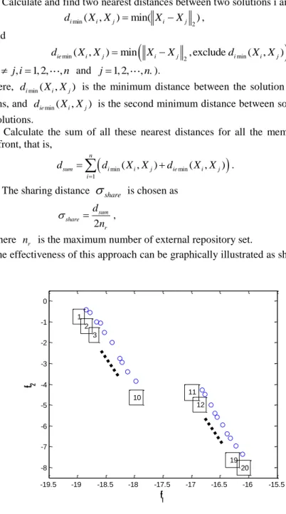
The effectiveness of this approach can be graphically illustrated as shown in Fig. 1. -19.5 -19 -18.5 -18 -17.5 -17 -16.5 -16 -15.5 -8 -7 -6 -5 -4 -3 -2 -1 0 f₁ f2 2 3 1 10 11 12 20 19

To calculate the sharing distance, the valid linear distance should be firstly calculated. For this example, there are 20 points and there is a gap between point 10 and 11. The real linear distance is the sum of the distance of two adjacent points, that is,

10 20 1, 1, 2 12     





x x . If the number of the members of the Pareto front set is properly chosen, the proposed adaptive sharing assessment scheme can make sure d_8,10d_10,11

and d_11,13d_10,11, and automatically reject the gap from the adjacent points, which means that the gap will not be considered by the proposed method as the distance between point 10 and point 11 is not the minimum or the second minimum distance. As all the information of the Pareto front set is used, it is more accurate than the existing methods; especially if the members of the Pareto front are numerous. For this example, the sharing distance is 0.34 using the real linear distance. Using the proposed method, the sharing distance is 0.41. The sharing distance is 0.43 using the method of Tan et al. [Tan, 11], which does not consider the gaps. According to our simulations, the sharing distance is very close to the sharing distance using real linear distance if the number of the members of the Pareto front set is large enough.

4

Adaptive sharing scheme based multi-objective PSO

These evidences by analogies are found in publications wherein multiple-swarm PSO is used to solve different optimization problems, particularly in multimodal problems [Iwamatsu, 06], [Seo, 06], and to counter PSO’s tendency in premature convergence [Yen, 08]. To improve the optimization performance, several multi-swarm PSOs were proposed in [Yen, 08], [Leong, 2008], [Cooren, 11] whose particle number is fixed or adaptive. However, they did not use the information of the obtained Pareto front to determine the searching areas/sub-spaces of sub-swarms. There is potential to achieve better results if some particles can search the areas around the achieved Pareto front during the search process, as most of the new Pareto front points are not far away from the old Pareto front points in the following iterations [Sun, 11]. In [Sun, 11], the fixed sharing distance and parameters were used, which limited the optimization performance since the shared distance cannot be accurately calculated. According to our investigation, if all the particles are too close to the Pareto front points, the global search ability will be limited. To avoid this disadvantage, some particles should be used to search other areas of the objective space and the Pareto front points should be properly chosen to allocate the sub-swarms.

Motivated by the above reviews, a new adaptive sharing scheme based MMPSO is proposed. The equations of the new method are similar with our previous proposed method in [Sun, 11], but the choice of the parameters are different and the new adaptive sharing scheme is used to improve the optimization performance in this study. Firstly, all the particles are divided into two types of sub-swarms: Pareto front sub-swarms, which are used to search different areas/regions around the proper chosen points of the Pareto front based on the proposed adaptive sharing scheme of Section 3; and Spare sub-swarms, which can be one sub-swarm or multiple sub-swarms and search the space(s) far away from the Pareto front. Without loss of generality only one sub-swarm is used for the spare sub-swarm in this study. This strategy can balance the global and

local search of all the particles in the objective space. The proposed method is based on the two types of sub-swarms, and there are two sets of the updating formulas based on these two different types of sub-swarms.

1) Pareto front sub-swarms: these Pareto front sub-swarms are used to search different areas around some properly chosen points of Pareto front; and the velocity and position updating equations are

(7)

(8) In the updating equations, there are three uniformly distributed random weightsR₁, R₂ and R₃in the range between 0 and 1, Core m( ) is the attraction point or the core of the

mth _{sub-swarm and determined by the proposed adaptive sharing so the diversity of the}

central points can be preserved. The mth _{sub-swarm is also dynamically determined}

according to the distance between the average position of every Pareto front sub-swarm and the mth _{core. The average position of the i}th ₍

max

{1, 2, , }

 i s ) sub-swarm and the

mth _{attract point are one-to-one correspondence for the minimum distance between}

them, then the ith _{sub-swarm will be the corresponding sub-swarm to the m}th _attract

point. Otherwise, one sub-swarm should be initialized around the mth _{attract point. If}

the number of the attract points is less than the maximum number of attract points, some Pareto front sub-swarms will be looked as part of the spare sub-swarm. c₃ can affect the attraction to the cores, and it should be chosen carefully. At the beginning the attraction can be some weak, and it should be stronger at the end of the optimization

procedure. Here the adaptive c₃ can be used, and in this study,

3 0.5 0.5* / max

c   iteration iteration where iteration is the current iteration and

max

iteration is the maximum number of iterations.

2) Spare sub-swarm: this sub-swarm consists of the remaining particles, and their updating equations are

(9)

(10) Here, R4 is a uniformly distributed random weight in the range [0, 1],c₄ is

variable parameter which is the value of the sharing function (2) based on the distance between particle i and its closest corresponding core particle m,

(11) and m_g is a predefined parameter and it is the number of Pareto front sub-swarms. It should be noted that the cores are the attract points in (7) and the cores become the repulsive points in (9).

To keep characteristic of fast convergence and avoid premature of PSO, a disturbance can be applied to a randomly chosen dimension of the velocity of the spare sub-swarm particles, and the formula can be described by

(12) whereR_v is a uniformly distributed random number between -1 and 1.

We are using the same method to determine P_i and P_g as the method in [Jeong, 09].

To realize this adaptive sharing scheme based multi-objective PSO, the follow steps can be used:

(1) Initialize the parameters, velocities and positions of the multi-objective PSO; (2) Calculate the fitness functions of particles.

Repeat:

(3) Determine the non-dominated Pareto front based on the adaptive sharing scheme and store the Pareto front points in the repository set.

(4) Based on the adaptive sharing scheme to choose the cores from the repository set for the Pareto front sub-swarms and dynamically construct the relationship among the sub-swarms and the cores.

(5) Using equations (7) and (8), or (9), (10) and (12) to update the velocities and positions of each particle.

(6) Calculate the fitness functions of particles. Until requirements are met.

5

Simulations and Analyses

In this section, six test famous multi-objective optimization problems are used to compare the performance of the proposed methods with the competing methods available in the literature.

5.1 Benchmark problems

The multi-objective optimization problems, which are typical in the literature, are ZDT1, ZDT2, ZDT3, ZDT6, Deb 2 and Viennet3, whose Pareto fronts are convex, non-convex & disconnected [Deb, 02], [Coello coello, 07].

1) ZDT1 Minimize f X₁( )x₁ (13) Minimize 1 2( ) ( ) 1 _{( )}    _  _   x f X g X g X (14) Here, X[ ,x x_{1 2}, ,x₃₀] ,







The Pareto front of this optimization problem is convex. 2) ZDT2

Minimize f X₁( )x₁ (15) Minimize 2 1 2( ) ( ) 1 _{( )}  _{ }   _{    }     x f X g X g X (16) Here, X[ ,x x_{1 2}, ,x₃₀] ,







The Pareto front of this optimization problem is non-convex. 3) ZDT3 Minimize f X₁( )x₁ (17) Minimize 1 1 2( ) ( ) 1 _{( )}- sin(10 1) ( )     _  _   x x f X g X _{g X} x g X (18) Here, X[ ,x x_{1 2}, ,x₃₀] ,







The Pareto front of this optimization problem is non-convex and disconnected. The real Pareto fronts of ZDT1, ZDT2 and ZDT3 are the objective value with

1[0,1] x and x_i0(i2, n). 4) ZDT6 Minimize 6 1( ) 1 exp( 4 )sin (6 1  1) f X x x (19) Minimize 1 2 2( ) ( ) 1 ( ) ( )    _  _   f f X g X g X (20) Here, X [ ,x x_{1 2}, ,x₁₀], 0.25 2 ( ) ( ) 1 9 9               



The real Pareto front is g x( )1and non-convex. 5) Deb 2 [Coello coello, 07]

Minimize f X₁( )x₁ (21) Minimize f X₂( )g X h X( ) ( ) (22) Here, X[ ,x x_{1 2}] , g X( ) 1 10x₂ , 2 1 1 1 ( ) 1 ( ) sin(12 ) ( ) ( )    f  f h X f

g x g x , xi[0,1] ( i1, 2.) . The Pareto front is

disconnected.

6) Viennet3 [Coello coello, 07]

Minimize f X₁( )0.5(x₁2x₂2) sin ( 2 x₁2x₂2) (23) Minimize 2 2 1 2 1 2 2 (3 2 4) ( 1) ( ) 15 8 27      x x  x x  f X (24)

Minimize ( 12 22) 3 2 2 1 2 1 ( ) 1.1 ( 1)      x x f X e x x (25) Here, X[ ,x x_{1 2}],xi [ 3,3] (i1, 2.).

The Pareto front of Viennet3 is three dimensional and is connected.

The Pareto front data of Deb2 and Viennet3 can be downloaded from http://www.cs.cinvestav.mx/~emoobook

To show the efficiency of the new method, the results from the new method are compared with the no-group method, which is also called single swarm method, and both of them are using the same parameters. The maximum number of fitness function evaluations is set to 50 000 and this is the unique stopping criterion. The swarm includes 200 particles for both methods. The maximum number of the first group sub-swarms is 8 and there are maximum 20 particles in each Pareto-front sub-swarm. For the test benchmark functions, the population are initialized 20 runs independently. The maximum number of members of the external repository set is set 100. We

setc₁ and are 2c₂ , and max

min min max ( ) )    loop i  loop max

（ where loop_max is the

maximum iterations; _max and _min are the maximum value and minimum value of inertia weight



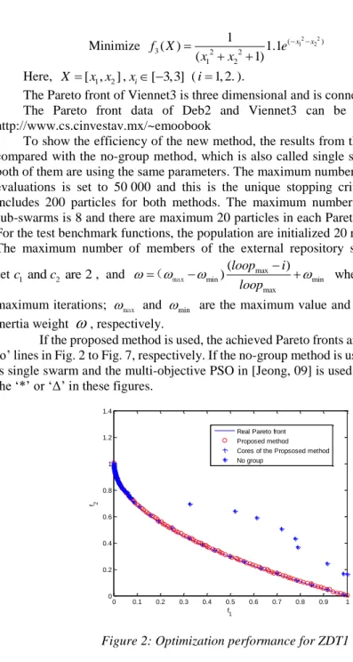
If the proposed method is used, the achieved Pareto fronts are shown by the red ‘o’ lines in Fig. 2 to Fig. 7, respectively. If the no-group method is used, which means it is single swarm and the multi-objective PSO in [Jeong, 09] is used, the Pareto front is the ‘*’ or ‘Δ’ in these figures.

0 0.1 0.2 0.3 0.4 0.5 0.6 0.7 0.8 0.9 1 0 0.2 0.4 0.6 0.8 1 1.2 1.4 f 1 f2

Real Pareto front Proposed method Cores of the Propsosed method No group

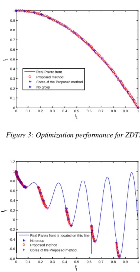
0 0.1 0.2 0.3 0.4 0.5 0.6 0.7 0.8 0.9 1 0 0.1 0.2 0.3 0.4 0.5 0.6 0.7 0.8 0.9 1 f₁ f2

Real Pareto front Proposed method Cores of the Proposed method No group

Figure 3: Optimization performance for ZDT2

0 0.1 0.2 0.3 0.4 0.5 0.6 0.7 0.8 0.9 1 -0.8 -0.6 -0.4 -0.2 0 0.2 0.4 0.6 0.8 1 1.2 f₁ f2

Real Pareto front is located on this line No group

Proposed method Cores of the Proposed method

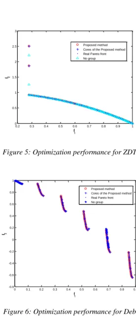
0.2 0.3 0.4 0.5 0.6 0.7 0.8 0.9 1 0 0.5 1 1.5 2 2.5 3 f₁ f2 Proposed method Cores of the Proposed method Real Pareto front No group

Figure 5: Optimization performance for ZDT 6

0 0.1 0.2 0.3 0.4 0.5 0.6 0.7 0.8 0.9 -0.8 -0.6 -0.4 -0.2 0 0.2 0.4 0.6 0.8 1 f₁ f2 Proposed method Cores of the Proposed method Real Pareto front No group

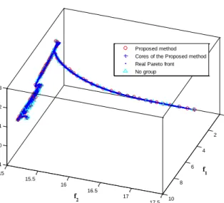
0 2 4 6 8 10 15 15.5 16 16.5 17 17.5 -0.1 0 0.1 0.2 0.3 f 1 f₂ f3 Proposed method Cores of the Proposed method Real Pareto front No group

Figure 7: Optimization performance for Viennet 3

As can be seen from Figs. 2, 3, 4, and 6, the adaptive Sharing Scheme based Sub-swarm Multi-objective PSO can achieve better performance than the no-group method. Moreover, the no-group method cannot find the complete Pareto fronts in Figs. 2, 3, 4 and 6 due to its premature. According to Fig. 5, the optimization performance of the proposed method is not good on the bound, but the results can be improved based on the optimization problem specifications such as rejecting some unreasonable results. It is difficult to compare their based on Figs. 5 and 7, and it would be better to use some performance metrics to compare their performance. The quantitative measures of Generational Distance and Spacing Metrics are discussed in the next section.

5.2 Pareto Front Performance Metrics

To quantitatively assess the performance of multi-objective optimizers, Generational Distance and Spacing metrics are two important metrics [Coello coello, 04], [Liu, 07], [Coello coello, 07].

1) Generational Distance (GD)

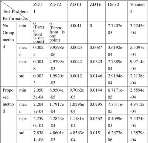
This metric gives a good indication of the gap between the discovered Pareto front and the real Pareto front [Coello coello, 04], and it is described by

2 1 n i i

d

GD

n





n

d

The GD comparison of the proposed method and the no group optimization method is shown in Table 1. Test Problem Performance ZDT 1 ZDT2 ZDT3 ZDT6 Deb 2 Viennet 3 No Group metho d min 0 _(Paret o front is one point) 0 (Pareto front is one point) 0.0011 0 7.7407e-05 3.2245e -04 mea n 0.002 3 9.9598e -06 0.0025 0.0087 3.6192e-04 5.5097e -04 max 0.004 8 4.9799e -05 0.0042 0.0343 7.7389e-04 9.9714e -04 std 0.002 3 1.9920e -05 0.0012 0.0146 2.9194e-04 2.2138e -04 Propo sed metho d min 2.050 5e-04 8.9504e -05 9.7062e -05 0.0144 6.7171e-05 2.5594e -04 mea n 2.204 7e-04 1.7917e -04 1.0296e -04 0.0295 7.7311e-05 4.9412e -04 max 2.259 0e-04 2.2823e -04 1.1181e -04 0.0562 8.4099e-05 7.2074e -04 std 7.836 1e-06 4.8601e -05 4.8563e -04 0.0151 6.2673e-06 1.3879e -04

Table 1: GD comparison of the proposed method and the no group optimization method

This metric is used to measure the distribution of vectors throughout the non-dominated vectors found so far [Coello coello, 04], and it is described by

2 1 1 ( ) 1 d i i S d d n    



i

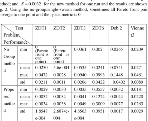
d , and n is the number of non-dominated vectors found so far. This metric shows how well the Pareto front found is, i.e. if all the points are on or very close to the real Pareto front. In general, the smaller the spacing metric is, the better the particles are spread along the Pareto front. At this situation, the smaller the spacing metric is, the better the particles are spread along the Pareto front. It is better to use the spacing metric together with the Pareto front figure since the spacing metric maybe not properly show the real optimization performance. For example, S0.038 for the no-group method; and S0.0032 for the new method for one run and the results are shown in Fig. 2. Using the no-group/single-swarm method, sometimes all Pareto front points converge to one point and the space metric is 0.

Test Problem Performance ZDT1 ZDT2 ZDT3 ZDT6 Deb 2 Vienne t3 No Group metho d min 0 _(Pareto front is one point) 0 (Pareto front is one point) 0.0361 0.002 0.0265 0.0209 mean 0.0230 5.6e-004 0.0535 0.0241 0.0741 0.0271 max 0.0472 0.0028 0.0940 0.0993 0.1448 0.0461 std 0.0211 0.0011 0.0206 0.0422 0.0402 0.0089 Propo sed metho d min 0.0029 0.0030 0.0035 0.0557 0.0032 0.0181 mean 0.0032 0.0034 0.0041 0.1224 0.0044 0.0220 max 0.0034 0.0038 0.0049 0.3009 0.0077 0.0263 std 1.8547 e-004 2.6874e-004 4.8563 e-004 0.0951 0.0017 0.0029

Table 2: Spacing comparison of the proposed method and the no group optimization method

From Tables 1 and 2, the new method can achieve improved Pareto fronts, except for ZDT6. It should be noted that in general the smaller GD and spacing measures show the better optimization performance if the members of the achieved Pareto front are distributed around the real Pareto front. However, the results of GD and spacing

measure maybe not properly show the real optimization performance especially the members of Pareto front converge to a very small space/area, for example, all the obtained members of Pareto front set converge to one point and the real Pareto front is lines or surfaces, which means the GD and spacing measure are zero but the optimization performance is not good such as the result for ZDT2 using the no group method. Hence we should also consider the figures to find whether the optimization performance is good or not when we are using GD and spacing measure.For ZDT6, the statistical results and Fig. 5 of the proposed method is not as good as some Pareto front points are on the bound, that is at the line of f₁0.2808, in the objective space. A similar situation occurred using the SPEA method as can be seen from Fig. 11 of reference [Deb, 02]. In general, the user’s choice and problem environment can also be used to choose a suitable set of Pareto front solutions. For ZDT6, we can delete some undesired points, for example, it maybe not acceptable if f₂ 1. The statistical results of the performance metrics are that the statistical results of GD all are zeros, and the statistical results of the spacing metrics are min = 0.0054, mean = 0.0083, max = 0.0171 and std = 0.0037; and these results are acceptable.

For the benchmark functions ZT1, ZT2 and ZT3, the average fitness values of the new method and one adaptive MOPSO [Cooren, 11] are (0.0032, 0.0034 and 0.0041) and (0.0047, 0.013 and 0.0336), respectively, which means the new method is more stable than the results from [Cooren, 11].

6

Conclusion

A new adaptive sharing scheme was proposed. Using this scheme, the sharing distance is stable and very close to the real linear distance if the members of Pareto front are numerous. The proposed adaptive sharing scheme can automatically identify the gap and the adjacent points, and the members of the Pareto front set can be evenly distributed according the simulation results, and this scheme is a general technique and can be used in other MOO algorithms. To improve the optimization performance, multiple sub-swarms have been dynamical used based on the information of Pareto front set. In general, the simulations showed that the proposed adaptive sharing scheme based multi-swarm multi-objective PSO can achieve better optimization performance comparing with no-group/single-swarm method and one adaptive multi-objective Particle Swarm Optimization, especially for the optimization problems whose Pareto fronts have gaps. Due to the good optimization performance of the proposed method, it can be applied in the multi-objective problems in Economics, Finance, Optimal control, Optimal design, Process optimizations, Electric power systems, and so on. Moreover, particle swarm optimization with adaptive population size and adaptive swarm size will be further investigated in the future.

Acknowledgments

Compliance with ethical standards

Conflict of interest I hereby and on behalf of the co-authors, declare all the authors agreed to submit the article exclusively to this journal and also declare that there is no conflict of interests regarding the publication of this article.

Ethical approval

This article does not contain any studies with human participants performed by any of the authors.

References

[Chen, 09] Chen D., Zhao C.: Particle swarm optimization with adaptive population size and its

application, Application Software Computation, 939-948, 2009.

http://www.sciencedirect.com/science/article/pii/S1568494608000318

[Coello coello, 04] Coello coello, C.A., Pulido, G.T., Lechuga, M.S.: Handling Multiple Objectives with Particle Swarm Optimization, IEEE Transactions on Evolutionary Computation, Vol. 8, No. 3, 256-279, 2004. http://ieeexplore.ieee.org/document/1304847/

[Coello coello, 07] Coello coello, C.A., Lamont, G.B., van Veldhuizen, D.A.: Evolutionary Algorithms for Solving Multi-Objective Problems, New York: Springer-Verlag, 2007. http://www.springer.com/gp/book/9780387332543

[Cooren, 11] Cooren Y., Clerc M., Siarry, P.: MO-TRIBES, an adaptive multiobjective particle swarm optimization algorithm, Computational Optimization and Application, Vol. 49, No. 2, 379-400, 2011. https://link.springer.com/article/10.1007/s10589-009-9284-z

[Deb, 02] Deb, K., Pratap, A., Agarwal, S., Meyarivan, T.: A fast and elitist multiobjective genetic algorithm: NSGA-II, IEEE Transactions on Evolutionary Computation, Vol. 6, No. 2, 182-197, 2002. http://ieeexplore.ieee.org/document/996017/

[Fonseca, 03] Fonseca, C.M., Fleming, P. J.: Genetic Algorithm for Multi-objective Optimization, Formulation, Discussion and Generalization. In Forrest, S. (ed.) Genetic Algorithms: In Proc. of the Fifth Int. Conf. on Genetic Algorithm, 1993, 416–423. San Mateo, CA: Morgan Kaufmann, 1993.

http://citeseerx.ist.psu.edu/viewdoc/download?doi=10.1.1.122.5689&rep=rep1&type=pdf [Goldberg, 89] Goldberg, D.E.: Genetic Algorithms in Search, Optimization and Machine Learning. Addison-Wesley: Reading, MA, 1989. http://dl.acm.org/citation.cfm?id=534133 [Ho, 05] Ho, S.L., Yang, S., Ni, G., Lo, E.W.C., Wong, H.C.: A particle swarm optimization-based method for multiobjective design optimizations, IEEE Transaction on Magnetics, vol. 41, no. 5, 1756-1759, May 2005. http://ieeexplore.ieee.org/document/1430958/ [Iwamatsu, 06] Iwamatsu, M.: Multi-species particle swarm optimizer for multimodal function optimization, IEICE Transaction Information System, Vol. E89D, no. 3, 1181-1187, 2006. http://search.ieice.org/bin/summary.php?id=e89-d_3_1181&category=D&year=2006&lang=E &abst=

[Jeong, 09] Jeong, S., Hasegawa, S., Shimoyama, K., Obayashi, S.: Development and Investigation of Efficient GA/PSO-Hybrid Algorithm Applicable to Real-World Design Optimization, IEEE Computational Intelligence Magazine, August, 36-44, 2009. http://ieeexplore.ieee.org/document/5190933/

[Kennedy, 95] Kennedy, J., Eberhart, R.C.: Particle Swarm Optimization, in Proceedings of IEEE International Conference Neural Networks, Perth, Australia, pp. 1942-1948, 1995. https://www.cs.tufts.edu/comp/150GA/homeworks/hw3/_reading6%201995%20particle%20sw arming.pdf

[Khor, 05] Khor, E.F., Tan, K.C., Lee, T.H., Goh, C.K.: A Study on Distribution Preservation Mechanism in Evolutionary Multi-Objective Optimization, Artificial Intelligence Review, Vol. 23, pp. 23:31-56, 2005. https://link.springer.com/article/10.1007/s10462-004-2902-3

[Leong, 08] Leong, W.F., Yen, G.G.: PSO-based multi-objective optimization with dynamic population size and adaptive local archives, IEEE Transactions Systems, Man, Cybern. B, Cybern, Vol. 38, No. 5, pp. 1270-1293, Oct. 2008.

http://ieeexplore.ieee.org/stamp/stamp.jsp?arnumber=4581390

[Liu, 07] Liu, D., Tan K.C., Goh, C.K., Ho, W.K.: A Multi-objective Memetic Algorithm Based on Particle Swarm Optimization, IEEE Transactions on Systems, Man, and Cybernetics-Part B: Cybernetics, Vol. 37, No. 1, 42-50, 2007.

http://ieeexplore.ieee.org/stamp/stamp.jsp?arnumber=4067074

[Miller, 96] Miller, B.L., Shaw, M.J.: Genetic Algorithms with Dynamic Niche Sharing for Multimodal Function Optimization. IEEE Int. Conf. on Evolutionary Computation, 786–791. Nagoya, Japan, 1996.

https://pdfs.semanticscholar.org/ae1a/2ced80613513115c3f851dc4dde95c792757.pdf

[Seo, 06] Seo, J.H., Lim, C.H., Heo, C.G., Kim, J.K., Jung, H.K., Lee, C.C.: Multimodal function optimization based on particle swarm optimization, IEEE Transactions on Magnetics, Vol. 42, No. 4, 1095-1098, April 2006. http://ieeexplore.ieee.org/document/1608401/

[Sun, 11] Sun, Y., van Wyk, B.J., Wang, Z.: A New Multi-swarm Multi-objective Particle Swarm Optimization based on a Pareto Front Set, the 2011 Int. Conf. on Intelligent Computing, Zhengzhou, China 11-14 August, Lecture Notes in Artificial Intelligence (LNAI), 6839: 203-210, 2011. https://link.springer.com/chapter/10.1007/978-3-642-25944-9_27

[Tan, 05] Tan, K.C., Khor, E.F., Lee, T.H., Heng, T.: Multiobjective Evolutionary Algorithms and Applications, New York: Springer-Verlag, 2005.

http://www.springer.com/gp/book/9781852338367

[Tan, 11] Tan, K.C., Khor E.F., Lee T.H., Sathikannan, R.: An evolutionary algorithm with advanced goal and priority specification for multi-objective optimization, Journal of Artificial Intelligence Research, 18, 183-215, 2011.

https://www.aaai.org/Papers/JAIR/Vol18/JAIR-1806.pdf

[Tian, 2017] Tian, Y. Cheng R., Zhang, X., Cheng, F., Jin, Y.: An indicator based multi-objective evolutionary algorithm with reference point adaptation for better versatility, IEEE Transactions on Evolutionary Computation, 2017, DOI 10.1109/TEVC.2017.2749619, in press. http://ieeexplore.ieee.org/document/8027123/.

[Yen, 08] Yen, G.G., Daneshyari, M.: Diversity-based information exchange among multiple swarms in particle swarm optimization, International. Journal Computer Intelligence Application, Vol. 7, No. 1, 57-75, 2008. http://ieeexplore.ieee.org/document/1688511/

[Yen. 03] Yen, G.G., Lu, H.: Dynamic multi-objective evolutionary algorithm: Adaptive cell-based rank and density estimation, IEEE Transactions on Evolutionary Computation, Vol. 7, No. 3, 253-274, Jun. 2003. http://ieeexplore.ieee.org/document/1206447/

[Yu, 08] Yu, B., Jiao, B., Gu, X.: Cooperative Particle Swarm Optimizer based on Multi-population and Its Application to Flow-Shop Scheduling Problem. In: 7th Int. Conf. on

Sys. Simulation and Scientific Computing, 1536--1542. IEEE Press, New York, 2008. http://ieeexplore.ieee.org/document/4675620/

[Zhang, 17] Zhang, L., Pan, H., Su, Y., Zhang, X., Niu, Y..: A mixed representation based multi-objective evolutionary algorithm for overlapping community detection, IEEE Transactions

on Cybernetics, Vol. 47, No. 9, 2703-2716. https://www.ncbi.nlm.nih.gov/pubmed/28622681.

[Zitzler, 01] Zitzler, E., Laumanns, M., Thiele, L., SPEA2: Improving the strength Pareto evolutionary algorithm, Computation Engineering Networks Lab. (TIK), Swiss Fed. Inst.

Technol. (ETH), Zurich, Switzerland, Tech. Rep. 103, May 2001.