Fast Algorithms for Monotonic Discounted Linear
Programs with Two Variables per Inequality
∗
Daniel Andersson
†and Sergei Vorobyov
‡§Uppsala University, Sweden
May 19, 2006
Abstract
We suggest new strongly polynomial algorithms for solving linear programs min(P
xi|S) with constraints S of the monotonic discounted form xi ≥ λxj +β
with 0< λ <1. The algorithm for the case when the discounting factor λis equal for all constraints isO(mn2), whereas the algorithm for the case whenλmay vary between the constraints is O(mn2logm), where n is the number of variables and
m is the number of constraints.
As applications, we obtain the best currently available algorithm for two-player discounted payoff games and a new faster strongly subexponential algorithm for the ergodic partition problem for mean payoff games.
1
Introduction
One of the most important open problems in mathematical optimization is the existence of a strongly polynomial algorithm for linear programming. In the (weakly) polynomial ellipsoid algorithm due to Khachiyan and the interior-point algorithms of Karmarkar, the number of operations depends not only on the number of variables n and constraints
m, but also on the magnitude of the coefficients. The quest for a strongly polynomial algorithm, with a running time polynomial inn,m, while independent of the coefficients, has continued for the last quarter of a century.
Particular cases of this fundamental problem appear in solving infinite games. For instance, the only currently known way to efficiently solve the one-player version of Shap-ley’s stochastic games [10] (or Markov decision processes) is by solving a linear program (with no known strongly polynomial algorithms). However, this program min(P
xi|S) has many special properties. The constraints of S are monotonic discounted, i.e., have form xi ≥ Pi6=jajxj +β, with 0 ≤ aj and Paj < 1. The feasible region contains a unique minimal element, which is also the solution to the program and the game.
∗Preprint NI06019-LAA, Isaac Newton Institute for Mathematical Sciences, Cambridge, United King-dom (http://www.newton.cam.ac.uk/).
†Supported by the Emma and Anders Zorn Foundation.
‡Support by the EPSRC Grant 531174 and by the VR Grant 50861101 is gratefully acknowledged. §Participant of the Logic and Algorithms Programme organized at the Isaac Newton Institute.
A few particular classes of linear programs allowing for strongly polynomial algorithms are known. For example, [4, 7] (see also references therein) give strongly polynomial algorithms for finding feasible solutions of arbitrary, not necessarily monotonic, linear programs with two variables per inequality.
In this paper we suggest new strongly polynomial algorithms for solvingto optimality1
a particular case of the above monotonic linear programs, consisting of MD2-constraints
(monotonic discounted 2-variable constraints). An MD2-constraint has the form xi ≥
λxj +β for some β, λ ∈ R with 0 < λ < 1 (a single variable constraint xi ≥ β can be expressed as xi ≥ λxi+β(1−λ)). An MD2-linear program consists in minimizing the sum of all variablesP
xi subject to a system of MD2-constraints in which every variable appears in the left-hand side of at least one constraint.2
We describe two different algorithms for two kinds of MD2-linear programs. First, in Section 3 we address the case when the discounting factorsλare equal for all constraints. The underlying idea of the algorithm seems to be new, although very natural and admit-ting an elegant runtime analysis. Staradmit-ting with a feasible solution, which is easy to find for MD2-constraints (linear time in the number of constraints), we consider trees defined by constraints tightly satisfied by the current feasible solution, i.e., xi =λxj+β (taking at most one per left-hand side variable). A variable not occurring on the left in any tight constraints is called a root. Pulling down the root of such a tree, by decreasing the values of all nodes while trying to preserve all tree equalities leads to either the disappearance of the root, or a defection of a subtree to another tree, or an internal switch, when a subtree reconnects in an alternative way within the same tree. Using a greedy strategy results in an O(mn2) algorithm, and the equality of discounting factors is essential for
the analysis, allowing to (tightly) bound the number of internal switches to the square of the initial number of tree nodes. This case covers the standard one-player discounted payoff games. When combined with the randomized techniques for two player games [2] (as a subroutine), it results in the best currently known subexponential algorithm for discounted payoff games. It also yields a new, more efficient, strongly subexponential algorithm for the ergodic partition problem for mean payoff games; see Section 5.
Second, in Section 4 we consider the case of different discounting factors. In this case it is possible to modify the algorithm of [7] for feasibility of two-variable systems of linear constraint for solving MD2-linear programs to optimality. The resulting bound for finding the optimum is O(mn2logm), the same as for the feasibility algorithm [7].
Relation to the Linear Complementarity Problem (LCP). An instance (A, b) of the LCP is given by a square matrix A ∈ Rn×n and a vector b ∈ Rn, and consists in finding a vector x ≥ 0 such that Ax+b ≥ 0 and xT(Ax+b) = 0 [8, 5]. Recall that a square real matrix is called: 1) a Z-matrix if its all off-diagonal elements are nonpositive; 2) a P-matrix if its all principal minors are positive (in particular, all diagonal elements are positive); 3) a K-matrix if it is simultaneously a Z- and a P-matrix. For a P-matrix
Athe LCP instance (A, b) has a unique solution for everyb. Chandrasekaran’s algorithm solves instances of the Z-matrix (hence, K-matrix) LCP problem in strongly polynomial time [5]. When A is a K-matrix, the unique solution found by the algorithm coincides with the least element of the feasible set S ={x≥0, Ax+b≥0}, or, equivalently, with
1
Note that feasibility for our systems of constraints can easily be found inO(m) time; see below. 2
the unique optimal solution of the linear program min(pTx|S) for any positive vector
p. Thus Chandrasekaran’s algorithm solves the above linear programs with square K-matrices in strongly polynomial time. Such linear programs are necessarily monotonic, i.e., each inequality has the form xi ≥pTx, with p≥0, and have at most two constraints with each variable on the left (with xi ≥ 0 being the second). A more general problem of strongly polynomial solvability of such systems when more than two constraints per variable on the left-hand side is open. This problem is equivalent to the so-called K-matrix Generalized LCP. Our paper solves a particular case of this more general problem, when constraints are monotonic, discounted, and contain at most one variable on the right of each constraint (or two variables per constraint).
2
Preliminaries
Throughout the paper we use the standard linear algebraic notation and conventions, e.g., assume that vectors are column vectors denoted by lettersx,y,z,a,b, etc. Corresponding indexed letters, like xi, denote vector coordinates, juxtaposition means vector scalar product, and xT denotes the transposition of vector x. We always let n denote the dimension of the underlying real vector spaceRn andm the number of linear constraints in the system under consideration. We tacitly assume that m ≥ n. Depending on the context, 1 can denote the all-ones vector h1, . . . ,1i ∈Rn.
Definition 2.1 (Monotonic Discounted Constraints) A vectora ∈Rnis called mo-notonic discounted (MD-vector) if it has a unique component equal to1, all its other com-ponents are nonpositive, and sum up to a number strictly greater than −1. A monotonic discounted constraint (MD-constraint) has the form aTx ≥ β for an MD-vector a ∈
Rn
and β ∈R.
An vector is an MD-vector with at most one negative component, and an MD2-constraint has the form aTx≥β for an MD2-vector a∈
Rn and β ∈R.
Thei-th groupSi of a system S of MD- or MD2-constraints consists of all constraints
aTx≥β of S in which the vector a has thei-th component equal to 1. A system S is full
if Si 6=∅ for each i∈ {1, . . . , n}. 2 The feasible region for an MD-system is always non-empty and we can easily find a feasible solution.
Proposition 2.2 A feasible solution for a given MD-system can be computed in O(mn)
time. For an MD2-system, O(m) time suffices.
Proof. Then-dimensional vector 1ξ =hξ, . . . , ξiis feasible for an MD-system iff for each constraint aTx≥β we have aT(1ξ)≥β or, equivalently, ξ≥β/(1Ta). Thus, taking ξ to be the maximum of β/(1Ta) over all constraints, makes 1ξ a feasible solution satisfying
at least one constraint as equality. 2
For two vectors x≤ymeans componentwise xi ≤yi for each i∈ {1, . . . , n}, and ≥is used correspondingly. A vector xis aleast element of the setX if x≤yfor every y∈X. The main problem we concentrate upon in this paper is the following.
MD2-Least Element Problem (MD2-LEP). Given: a full system S of MD2-constraints.
Find: the least element of the convex polyhedron defined by S. 2
This least element always exists and is uniquely defined, which follows from Proposi-tion 2.3, summarizing well-known elementary properties of MD-systems.
For a full system of MD-constraints S call S′ a representative subsystem of S if S′
contains exactly one constraint of S per group. A representative equality subsystem is a representative subsystem in which all inequalities ≥ are replaced with equalities =. By discountedness, each such subsystem has a nondegenerate matrix, hence possesses a unique solution.
Proposition 2.3 Let S be a full system of MD-constraints.
1. If x and y are feasible for S then z, defined by zi = min(xi, yi) for i ∈ {1, . . . , n},
is also feasible for S.
2. If S contains one constraint per group then the unique solution x∗ of its unique representative equality subsystem is the least element ofS andx∗ = arg min(1Tx|S).
3. z = arg min(1Tx|S) is finite.
4. z = arg min(1Tx|S) satisfies at least one constraint in each group as equality.
5. z = arg min(1Tx|S) coincides with the unique solution to one of the representative
equality subsystems of S.
Proof.
1. Choose any constraint aTu≥β fromS. Suppose w.l.o.g. that a
1 = 1 and z1 =x1.
Note that aTx = aThz
1, z2 +δ2, . . . , zn+δni ≥ β, where zi +δi = xi and δi ≥ 0 for i ∈ {2, . . . , n}, implies aTz ≥ β, because the components a
i for i ∈ {2, . . . , n} are nonpositive. Indeed, aTx= aThz
1, z2 +δ2, . . . , zn+δni =aTz+Pni=2aiδi ≥ β impliesaTz ≥β, since the sum is nonpositive.
2. Let x be a feasible solution of S ≡ Ax ≥ b and let x∗ be the unique solution of Ax = b. Then A(x−x∗) ≥ 0 and x−x∗ ≥ 0 (or x ≥ x∗) easily follows. Indeed,
assuming x6≥x∗, select the smallest negativex
i −x∗i and get a contradiction with the discountedness of A.
3. Choose any representative equality subsystemS′ ofS, and letx∗ be its unique finite
solution. Since S′ is a subsystem of S it follows thatz is feasible for S′, so by 2 we
have x∗ ≤z.
4. Otherwise, z would not be a minimum (if all inequalities in Si were strict, then zi could be decreased).
Corollary 2.4 For a full system S of MD-constraints there is a unique least element in the convex polyhedron defined by S, which coincides with the unique optimal solution to the linear program min(pTx|S), where p is any positive vector. 2 We now sketch the two simple methods of computing least elements of full MD-systems, both based on Proposition 2.3. The first one is straightforward. It suffices to find a representative equality subsystem with the unique solution (found by Gaus-sian elimination) being a feasible solution to the whole system. This can be done by a straightforward exhaustive search in time O((n3+m)·Πn
i=1ni), where ni is the number of inequalities for thei-th variable (the size of the i-th group).
A less straightforward method is to fix a representative equality subsystemS′ and find
its unique solution x′. If x′ satisfies all other constraints of the system, it is the required
least element. Otherwise, takeany violated constraint and use it instead of the constraint in S′ from the same group. The new unique solution x′′ of the resulting representative
equality subsystem is in the feasible region ofS′(considered as inequalities≥), of whichx′
is the least element. Therefore, x′ < x′′, which guarantees monotonicity and termination.
However, the worst case bound remains the same. Below we will suggest more efficient methods for MD2-linear programs.
2.1
Two Types of MD-Systems
Due to the asymmetry of the discounting factors (negative components of a), we need to distinguish between two types of MD-systems: the ≥-type, defined above, and the
≤-type, which differs from the above by reversing the direction of all inequalities.
The full ≥-type MD-systems are appropriate for the problem of finding the least element of the feasible region, which coincides with the problem of finding the unique minimum of the function 1Tx on the feasible region.
Symmetrically, the full≤-type MD-systems are appropriate for the problem of finding the greatest element of the feasible region, which coincides with the problem of finding the unique maximum of the function 1Tx on the feasible region.
These problems are however easily reducible to each other, since Ax≤b iff A(−x)≥
−b. Thus it is sufficient to give algorithms for solving the ≥-type problem, as we will do in the remainder of this paper.
We also have the following simple, but useful, connection.
Proposition 2.5 If x is feasible for a full ≥-type MD-system and y is feasible for the reversed system, then y ≤x.
Proof. Choose any representative equality subsystem, and let z∗ be its unique solution.
3
Equal Discounting Factors
We first consider the case of MD2-LEP when the constraints have equal discounts, i.e., there is a single discounting factor λ, where 0 < λ < 1, and all constraints are of the form xi ≥ λxj +βij (if i =j then this is equivalent to xi ≥ βii/(1−λ)). For this case, we may assume that there is at most one constraint per ordered pair of variables. In the following, we assume that xis a feasible solution to the full system of constraints.
Consider the weighted directed graph G with the variables of the constraint system as vertices, where a constraintxi ≥λxj+βij is represented by an edge fromxi toxj with weight βij. An edge is called tight if the corresponding constraint is satisfied as equality. Tight edges may be colored red, but at most one outgoing red edge per vertex is allowed. A vertex with no outgoing red edge is called a root.
Proposition 3.1 If every vertex has an outgoing red edge (i.e., there are no roots), then x is the unique minimal solution of the constraint system.
Proof. Follows from Proposition 2.3. 2
This suggests the following approach: starting from a feasible solution, we move in a nonpositive direction within the feasible region, making sure the number of red edges is nondecreasing. This has a clear intuitive interpretation as pulling a red tree down by its root, as explained below.
Definition 3.2 Ared zone is a maximal subgraphG′ of Ginduced by red edges such that for every two vertices u, v of G′ there is a vertex ofG′ reachable from bothuand v by red paths (possibly empty) in G′. Every red zone is either a red tree with a root (as defined above), or a red sun with a unique cycle and incoming rays.
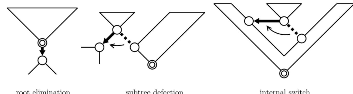
Definition 3.3 A pull-down of a red tree is performed as follows. The coordinates of x corresponding to nodes in the tree are decreased in such a way that the tree edges remain tight, while all other coordinates are kept fixed, until some constraint is just about to be violated. An edge corresponding to such a constraint (satisfied as equality) is then chosen, and is made the unique new outgoing red edge from its tail.
Note that the tail of this new red edge will always be a node originating from the red tree that was pulled down, due to the monotonicity of the constraints. Also, roots are never created, i.e., once a vertex has acquired an outgoing red edge, it will always have
some outgoing red edge. Thus, a pull-down results in one of the following three events, illustrated in Figure 1.
1. The root is eliminated, i.e., the whole tree grafts into a red zone (possibly itself, thereby creating a sun). This decreases the number of red trees by one.
2. A proper subtree defects, i.e., the new outgoing red edge of some non-root node connects the node and its predecessors to another red zone.
3. A non-root node makes an internal switch, i.e., reconnects within the same tree. Intuitively, this may happen for the following reason (formalized in Proposition 3.4). Every nodexiin a red tree is expressible as a linear functionxi =λkxj+β of its root
xj with the slope λk. By pulling the root down (decreasing xj), we also decrease
xi. At some point, a non-red edge between two nodes in the red tree may become tight and create an alternative path giving rise to the new function xi =λlxj +β′ with a smaller slope (the necessary condition for intersection), i.e., l > k, and an internal switch occurs.
Figure 1: The possible results of a pull-down operation.
Algorithm 1, given in pseudo-code below, starts with a feasible solution (lines 2–3) and no red edges (line 4), and then repeatedly chooses a root and eliminates it by repeated pull-downs (lines 9–20), until no roots remain. By Proposition 3.1, this will yield the unique minimal solution, provided the algorithm terminates. We will now prove that it does terminate, and also derive an upper bound on its running time.
Proposition 3.4 If an internal switch occurs, then the depth of the switching node in-creases.
Proof. During a pull-down, the feasible solutionxis moving in the direction−sfor some nonnegative vectors. We will callsi thespeed ofxi, and normalizesby making the speed of the root equal to 1. In order to keep a tree edge from xi to xj tight, we must have
si =λsj, hence the speed of any tree node xi must be λdepth ofxi. For any vertex xi not in the tree, we have si = 0.
Consider an edge from a tree node xi to a tree node xj, and suppose that the depth of xi is strictly greater than the depth of xj. Then si ≤ λsj, and, since x is feasible, we have xi ≥λxj+βij. This implies (xi −τ si)≥λ(xj −τ sj) +βij for any non-negative τ, i.e., the constraint will never be violated.
Thus, before an edge from xi toxj is colored red due to an internal switch, the depth of xi must be less or equal to the depth of xj, hence the switch increases the depth ofxi.
2
Corollary 3.5 The number of successive pull-downs needed to eliminate the root of a red tree is at most t2, where t is the number of nodes in the tree before the first pull-down.
Proof. By Proposition 3.4, a node can perform at most t−1 internal switches, and at
Algorithm 1: Solves MD2-LEP with equal discounting factors.
Input: An MD2-system represented by a weighted graph G = (V, E, w) and a discounting factor 0< λ <1. An edge (xi, xj)∈E ⊆V2 represents the linear constraintxi ≥λxj+w(xi, xj).
Output: The least element of the feasible region of the input system.
MD2=-Least-Element(V, E, w, λ)
(1) Compute a feasible solution.
(2) ξ ←maxe∈E
w(e) 1−λ
(3) value[V]←ξ
(4) color[E]←black
(5) while there is a root r of a smallest red tree
(6) Eliminate r.
(7) while r is the root of a red treeT
(8) Pull down T.
(9) VT ←nodes of T
(10) speed[V]←0
(11) foreach v ∈VT by pre-order tree traversal (12) speed[v]←λdepth ofvinT
(13) ET ← black outgoing edges from VT
(14) time[ET]← ∞
(15) foreach (u, v)∈ET
(16) if speed[u]> λ·speed[v]
(17) time[(u, v)]← λ·value[v]−value[u] +w(u, v) λ·speed[v]−speed[u] (18) (u, v)←arg mine∈ETtime[e]
(19) foreach x∈VT
(20) value[x]←value[x]−speed[x]·time[(u, v)] (21) color[outgoing edges from u]←black
(22) color[(u, v)]←red
(23) return value
The bound in Corollary 3.5 is asymptotically tight — it is possible to give an example when Θ(t2) pulls down are needed to eliminate one root, as will be done below.
Corollary 3.5 immediately yields an O(n3) upper bound on the total number of
pull-downs needed to eliminate all roots. However, we will now prove that, by using a greedy
strategy, always selecting the root of the smallest tree to be eliminated, just O(n2)
pull-downs suffice.
Proposition 3.6 By using the greedy strategy, all roots can be eliminated using O(n2)
pull-downs.
Proof. We always eliminate the root of the smallest tree. If there are k trees, at least one of them must have at most⌊n/k⌋ nodes, and thus the total number of pull-downs is
bounded above by n X k=1 n k 2 ≤n2 ∞ X k=1 1 k2 = π2n2 6 , which is O(n2). 2
A single pull-down operation is performed by the algorithm in O(m) time as follows. First, the speeds (of decrease) for all vertices are computed (lines 10–12). Then, for each outgoing edge from a tree node, the algorithm determines whether the edge would ever be violated (line 16), and if so, calculates time until it this would happen (line 17). Finally, an edge with the minimal time until violation is chosen (line 18), the values of tree nodes are decreased, and edge colors are updated.
This results in the following
Theorem 3.7 The running time of Algorithm 1 is O(mn2).
Proof. By Proposition 3.6, since a single pull-down operation is performed inO(m) time.
2
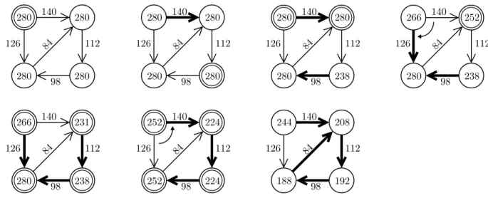
A sample run of Algorithm 1 is given in Figure 2. It illustrates an important property: an edge may become red more than once. If this had not been the case, then an O(m) bound on the total number of pull-downs would easily have followed.
Figure 2: Step by step illustration of the pull-downs performed by the algorithm on a particular input with λ = 1/2. Marked vertices are nodes of the red tree chosen for the next pull-down.
The worst-case running time of Algorithm 1 is in fact Θ(mn2), since it is possible
to construct inputs of any size for which the algorithm proceeds as follows.
First, a single red tree spanning the entire graph is grown. It consists of a chain of k
vertices x1, . . . , xk connected by red edges of weight 0 and another k vertices y1, . . . , yk connected by red edges with weightsβj1 to the root vertexx1. There are also black edges
has a black self-loop. We illustrate in Figure 3, for simplicity, the case k = 3, which straightforwardly generalizes to any k.
Pulling down the rootx1causes the value ofyj to decrease according toyj =βj1+λx1.
An internal switch occurs when the linear functionyj =βj1+λx1intersectsyj =βji+λix1
with i > 1, and yj “jumps” up the chain, because the slope λi is less steep than λ. The algorithm terminates when the self-loop ofx1 becomes tight.
By choosing suitable weights, we can guarantee that the value of each yj during the pull-downs will be a piecewise linear function of x1 consisting of k pieces with slopes λl
for decreasing l =k, . . . ,1. This will cause all vertices yj to climb the chain one level at
a time and result in a total of Θ(k2) = Θ(n2) internal switches.
x1 x2 x3 y1 y2 yy33 β j1+λx1 βj2+λ2x1 βj3+λ3x1 j = 1 j = 2 j = 3
Figure 3: A total of 6 internal switches can occur as the yj climb the chain.
4
Different Discounting Factors
In this section we address the case when constraints may have different discounting fac-tors. Proposition 3.4 requires equal discounts, and although lifting this assumption still leaves us with a variant — the product of discounts on the path to the root decreases — and thereby a proof of termination, it spoils the strongly polynomial bounds. Therefore, we use a different method for this case, at the cost of slightly worse time complexity.
Hochbaum and Naor [7] suggested a simple and fast deterministic O(mn2logm)
algo-rithm for finding a feasible solution of any linear system with at most two variables per inequality. We will show how to modify their algorithm so that it can be used to solve our optimization problem MD2-LEP.
The algorithm in [7] is based on the Fourier-Motzkin elimination method [9]. To eliminate a variablexi, all inequalities containingxi are replaced with inequalities L≤U for each pairL≤xi andxi ≤U in the original system. Feasibility is obviously preserved, and the method can be applied recursively to compute a feasible solution, or determine that no one exists. However, the number of inequalities created during this process may be exponential.
In [7] the growth of the number of inequalities during the repeated Fourier-Motzkin elimination is controlled by removing a lot of inequalities, and adding a few, in a way that preserves feasibility. This is done by searching for feasible values between breakpoints (defined below).
For any two distinct variables xi and xj, the feasible region of the subsystem of inequalities containing only xi and xj lies between an upper and lower envelope, which are piecewise linear functions in thexixj-plane. We denote the set of breakpoints of these functions by B(xi, xj).
The original algorithm is focused on finding anyfeasible solution. Feasibility is trivial in our case, and the algorithm must be modified. We now state the modified version, and refer the reader to [7] for a detailed description of the original algorithm.
4.1
Algorithm 2
For each variable xi, we denote by xmin
i the smallest value of xi in any feasible solution to the original system of inequalities. By Proposition 2.3, hxmin
1 , . . . , xminn i is the unique minimal element of the feasible region. Using Proposition 2.5 and 2.2, we compute values
ai and bi such thatai ≤xmini ≤bi, and add the inequalities ai ≤xi ≤bi to the system. We then perform steps(i)–(iv)for i= 1, . . . , n−1 and maintain the following invari-ant: before the i-th iteration, hxmin
i , . . . , xminn i is a feasible solution to the current set of
inequalities.
(i) Let B = hb1, . . . , bki be the sorted sequence of xi-coordinates of the breakpoints
S
i<j≤nB(xi, xj).
To maintain the invariant, we must make sure that xmin
i remains a feasible value for xi after step (iii).
(ii) Using the procedure of Aspvall and Shiloach [1] (which, given any valueα, decides if
α < xmini ), perform a binary search inBto findblandbl+1such thatbl ≤xmini ≤bl+1
(if there is no bl such thatbl < ximin, we must have xmini =b1).
(iii) Add the inequalities bl ≤xi and xi ≤bl+1, and discard any redundant inequalities.
For any xj, there will now be at most two inequalities containing xi and xj. (iv) Apply the Fourier-Motzkin elimination method to xi.
Since Fourier-Motzkin elimination preserves feasible ranges for the remaining variables, the invariant is preserved.
After n − 1 iterations of steps (i)–(iv), what remains is xn and two inequalities
α ≤ xn and xn ≤ β, where α and β are constants. By the invariant, we have α =xminn , and thus we assignαtoxn. Backtracking, i.e., restoring previously discarded inequalities containing xn−1 and xn, we assign to xn−1 the minimum feasible value with respect to
these inequalities and the value assigned to xn. By the invariant and monotonicity, continuing in this fashion for xn−2, . . . , x1 gives us the optimal solution.
Our modifications do not significantly affect the worst case analysis in [7], and this results in
5
Applications
Solving the MD2-LEP has the following obvious optimal control interpretation. Starting in a statexi, an agent selects one of a few available actions. Depending on the choicej, he gets paid some amountβ and causes some inflation rate λ, and the next day everything repeats from the state xj, ad infinitum. An optimal agent’s strategy is described by the MD2-LEP instance with constraints xi ≥β+λxj defining the possible actions.
5.1
Two-Player Discounted Payoff Games
The model above is also known as a one-player discounted payoff game (DPG). The two-player version of a DPG also has a second two-player who, alternating the actions with the first one, tries to make the payoff as small as possible. Such games are known to be solvable in pure positional (memoryless) strategies for both players [10].
Algorithm 1 from Section 3, when combined with the randomized combinatorial opti-mization game techniques [2], provides for the best currently available algorithms for the two-player DPGs.
Theorem 5.1 A two-player DPG can be solved in randomized subexponential time mn2·min f(nmax, mmax), f(nmin, mmin)
, (1)
where
f(n, m) =e2√nln(m/√n)+O(√n+lnm) (2)
and nπ, mπ is the number of vertices and edges of player π ∈ {min,max}. 2 Algorithm 2 gives a similar bound for the case of a generalized DPG, with different discounting factors. For previous algorithms, the bound was roughly the square of (1), more precisely, f(nmax, mmax)·f(nmin, mmin).
5.2
Ergodic Partition for Mean Payoff Games
We also obtain a new strongly subexponential algorithm for solving the ergodic partition
problem for mean payoff games (MPG): given an MPG find a partition of its vertices into subsets with equal values, together with their values [6].
Note that the algorithm from [3] is not strongly subexponential, it has a bound of the form log(W)·2O(√nlogn), where W is the maximum absolute edge weight. The latter
algorithm proceeds by bisecting the range of possible values (hence the factor logW), each time solving an instance of the longest shortest paths problem (in strongly subexponential time). Now we can give a strongly subexponential algorithm.
Theorem 5.2 The MPG ergodic partition problem can be solved in randomized strongly
subexponential time (1). 2
Proof. Reduce an MPG instance to a DPG instance, as in [11]. This reduction does not change the game graph, just adds an appropriately selected discounting factor. Finding values of this DPG can be done as explained in the previous section. The MPG values may be recovered from the DPG values. As a by-product, this algorithm also computes
6
Conclusions
Motivated by applications to one- and two-player games, we constructed two new strongly polynomial algorithms for finding unique optimal solutions to system of linear 2-variable monotonic inequalities, running in timeO(mn2) andO(mn2logm) for equal and different
discounting factors, respectively. Interestingly, there remains a big gap between finding feasible solutions to such systems in O(m) time and solving them to optimality. Also our algorithm for different discounting factors does not improve3 asymptotically over the
feasibility algorithm [7] for arbitrary 2-variable constraints. Designing new, more efficient algorithms to narrow the existing gaps, or “proving” natural lower bounds represent challenging algorithmic problems. Note that our equal discounts algorithm, incidentally, has the same complexity as Bellman-Ford’s shortest paths algorithm run from each vertex. Extending the techniques to solve, in strongly polynomial time, MD-linear programs, with no restriction on the number of variables per inequality, is another challenging problem, with important consequences for linear programming, game theory, and linear complementarity.
References
[1] B. Aspvall and Y. Shiloach. Polynomial time algorithm for solving systems of linear inequalities with two variables per inequality. SIAM J. Comput., 9:827–845, 1980. [2] H. Bj¨orklund and S. Vorobyov. Combinatorial structure and randomized
subexpo-nential algorithms for infinite games. Theoretical Computer Science, 349(3):347–360, 2005.
[3] H. Bj¨orklund and S. Vorobyov. A combinatorial strongly subexponential strategy improvement algorithm for mean payoff games. Discrete Applied Mathematics, 2006. Accepted for publication, to appear.
[4] E. Cohen and N. Megiddo. Improved algorithms for linear inequalities with two variables per inequality. SIAM J. Comput., 23(6):1313–1347, 1994.
[5] R. W. Cottle, J.-S. Pang, and R. E. Stone. The Linear Complementarity Problem. Academic Press, 1992.
[6] V. A. Gurvich, A. V. Karzanov, and L. G. Khachiyan. Cyclic games and an al-gorithm to find minimax cycle means in directed graphs. U.S.S.R. Computational Mathematics and Mathematical Physics, 28(5):85–91, 1988.
[7] D. S. Hochbaum and J. Naor. Simple and fast algorithms for linear and integer programs with two variables per inequality. SIAM J. Comput., 23(6):1179–1192, 1994.
[8] K. G. Murty and F.-T. Yu. Linear Complementarity, Linear
and Nonlinear Programming. Heldermann Verlag, Berlin, 1988. http://ioe.engin.umich.edu/people/fac/books/murty/linear complementarity webbook/.
3
[9] A. Schrijver. Theory of Linear and Integer Programming. John Wiley and Sons, 1986.
[10] L. S. Shapley. Stochastic games. Proc. Nat. Acad. Sci. USA, 39:1095–110, 1953. [11] U. Zwick and M. Paterson. The complexity of mean payoff games on graphs. Theor.