Introduction to Statistical Physics (2SP)
Richard Sear
March 15, 2011
Contents
1 What is the entropy (aka the uncertainty)? 2
1.1 One macroscopic state is the result of many many microscopic states . . . 2 1.2 States with equal energies are equally probable . . . 4 1.3 States with different energies: the role of Temperature . . . 4
2 The two-level system 6
3 Fluctuations and the Central Limit Theorem of Statistics 7
4 States with different numbers of particles 9
5 Fermi-Dirac and Bose-Einstein Statistics 10
5.1 A single level with Fermi-Dirac statistics . . . 11 5.2 A single level with Bose-Einstein statistics . . . 11 6 Averages and the relationship between the partition function and thermodynamic
quantities 13
6.1 Averages . . . 13 6.2 Average quantities at constant T . . . 13 6.2.1 The partition function Z and the Helmholtz free energyA . . . 14
7 Classical Statistical Mechanics 15
7.1 Example . . . 16 7.2 The equipartition theorem . . . 17 7.3 When is a gas classical and when are quantum mechanical effects important . . . 18
Recommended textbooks
I recommend four:
1. Statistical Mechanics: A Survival Guideby A. M. Glazer and J. S. Wark (Oxford). 2. Cencepts in Thermal Physicsby S. J. Blundell and K. M. Blundell (Oxford).
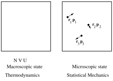
N V U
Thermodynamics Statistical Mechanics Macroscopic state Microscopic state
r p r p r p 1 2 3 1 2 3
Figure 1: Schematics of a gas or argon atoms from the viewpoint of thermodynamics (left-hand side) and from the viewpoint of statistical mechanics (right-hand side). In thermodynamics, we just deal with a handful of, macroscopic, properties, such as the total number of particles, N, volume V and total energy U. In statistical mechanics, we deal with microscopic states. For the gas of argon atoms the microscopic state is specified by the positions and momenta (or velocities) of all N argon atoms. We have only shown 3 atoms here. r1 is the position vector of atom 1,p1 is the momentum vector of
atom 1, r2 is the position vector of atom 2, and so on. The arrows indicate the momentum vectors,
and the dots are the positions of the atoms.
3. Introduction to Modern Statistical Mechanicsby D. Chandler (Oxford). 4. Introduction to Statistical Physics by K. Huang (Oxford).
3 goes a bit faster than either 1, 2 or 4. All four are in the library.
1
What is the entropy (aka the uncertainty)?
We will start off by looking at the most basic function in thermodynamics, and in statistical mechanics, the entropy, using a statistical description. You have already encountered the entropy in thermody-namics. The second law of thermodynamics is that at thermodynamic equilibrium the entropy is at a maximum. Note: a) thermodynamics does not tell you how to calculate the entropy of say, a given amount of steam. As we will see, statistical physics does allow you calculate the entropy. Also, b) recall that thermodynamics deals with large amounts of air, steam, iron etc, i.e., Avogadro’s number of atoms or molecules, 1024
, not one or a handful of molecules.
1.1
One macroscopic state is the result of many many microscopic states
Consider a gas, say, of N molecules, in a volume V and with an energy U. The gas has just one macroscopic, or thermodynamic, state but a huge number of possible states of its molecules. If a gas has N = 1024
molecules then the microscopic states of the gas are specified by the positions and momenta of all these N molecules. Whenever a molecule moves it changes its position and so the microscopic state of the system. Also, whenever it collides with another molecule, its velocity and
hence momentum will change and this too changes the microscopic state of the gas. See Fig. 1 for an illustration of the macroscopic and microscopic states of a gas.
This is for a gas of molecules that can be treated as classical objects, i.e., like billiard balls. For a quantum mechanical system, the microscopic state of a system is specified by specifying the quantum mechanical state the system is in. The possible states you get from solving Schr¨odinger’s equation. For example, a hydrogen atom will have two ground states, the 1s state with up and down spins, excited states, 2s, 2p etc. If we have two atoms then one could be in the 1s state, the other in a 2p state etc., while with three atoms we could have one in the 1s state, another in the 2p state and the third in the 2s state etc. Thus again if we have 1024
H atoms there are huge number of possible microscopic states of these atoms, corresponding to all the possible different electronic states the atoms can be in.
So, we have a huge number of states and typically we don’t know what the microscopic state of the system is. This is because to know this we would need to know the individual states of a huge number of molecules, and we would have to measure all these states very quickly, as as soon as a molecule moves or collides then the microscopic state changes.
This is completely impractical so we need to resort to statistics. Instead of trying to work out what the microscopic state is we will just assume each microscopic state occurs with a given probability, i.e., that the probability that we observe the system in the microscopic state numberi, is pi.
Here, we will calculate the entropy from Shannon’s equation. This was derived by Claude Shannon a little after the second world war. Shannon said that if we knew all probabilitiespi of all
S = −PN
i=1pilnpi
entropy of one macroscopic state sum overN microscopic states (1) wherepi is the probability of theith microscopic state, and the sum is overallthe possible microscopic
states. Note that here a macroscopic quantity, the entropy on the left-hand side, is given by a sum overmicroscopic quantities, the probabilities pi, of the microscopic states of the system.
Statistics is required to calculate thermodynamic properties such as the entropy, energy etc because each macroscopic or thermodynamic state is the result of many many microscopic states and we don’t know which microscopic states the system is an any instant, all we know is the probability that the system is in a given microscopic state (below we will see how to calculate these probabilities). So we need to work with probabilities, which requires statistics. For example, if I tell you that there is say a volume 1cm3
of steam with an energy of 1MJ, and a total number of water molecules of 1020
, which is all that is known and considered in thermodynamics, then you would not know what microscopic state the system is in. In order for you to know the microscopic state of the system I would have to tell you the position and momentum etc., of every molecule in the vapour. This is illustrated in Fig. 1. As with the information that thermodynamics provides, N, V and U, you do not know what the microscopic state is, then you have to make a guess and this inherently involves probabilities. We have to use probabilities because we do not know the exact microscopic state. Indeed the number of microscopic states is enormous and the system goes from one to another very rapidly as the particles move around, as the momenta are changed by collisions etc.. This lack of knowledge of the exact microscopic state is why this course is called statistical physics.
Note on units As defined by Eq. (1) the entropy S is just a pure number: it has no units. In thermodynamics in particular, entropy is often defined so that it does have units, generally JK−1
. In this course we will always use entropies defined so that they are dimensionless, as in Eq. (1). The entropies used in your thermal physics course, with units of JK−1
are obtained by multiplying the entropies here by Boltzmann’s constant k = 1.38×10⁻²³
JK−1
1.2
States with equal energies are equally probable
If different states (with the same number of particles) have the same energy, then there is no reason for them to have different probabilities. Thus, we assume that states with the same energy have the same probability. For example, consider a system with two states, call them states 1 and 2. If they have the same energy then they are equally probable, i.e., the probability that the system is in state 1, p1,
equals the probability that the system is in state 2,p2. As probabilities must add to one, p1+p2 = 1
and so as p1 =p2, then both p1 and p2 are equal to 1/2. Thus the entropy is of the simple system is
S=−p1lnp1−p2lnp2 =− 1 2ln 1 2 − 1 2ln 1 2 =−ln 1 2 = ln 2 (2)
Here the entropy is just equal to the log of the number of states, 2. In fact in general if a system has not 2 microscopic states but Ω states with equal energies then all these Ω states will be equally probable. The probability of each state is then just 1/Ω, and the the entropy is
S = − Ω X i=1 pilnpi =− Ω X i=1 1 Ωln 1 Ω =−Ω1 Ωln 1 Ω =−ln 1 Ω (3) S = ln Ω (4)
where we used the fact that the sum is of Ω terms all of which are the same. So, we see that in general when all the microscopic states are equally probable, that the entropy is just the log of the number of states. As a gas has something like exp(1023
) states not 2. The equation S = ln Ω is Boltzmann’s equation for the entropy, for states all with the same energy. It is in fact on his tombstone in Vienna. Boltzmann’s equation predates that of Shannon, but is less general.
The entropy is sometimes called the uncertainty, and we can see why from Eq. (4). As the number of states, Ω, increases, our uncertainty as to which state the system is in increases. If Ω = 10 then the system could be in 1 of 10 states, but if Ω = 10,000, then the system could be in any 1 of 10,000 states. Thus, as Ω increases so does our uncertainty as to which state the system is actually in.
1.3
States with different energies: the role of Temperature
Most often the microscopic states of a system do not all have the same energy. Then the system will have some average energy U, which depends on the probabilities of the system being in the different microscopic states with different energies. By definition the average energyU is the sum over all states with each state contributing its energy times the probability that the system is actually in that state. So,
U =X
i
piǫi definition (5)
where ǫi is the energy in statei.
So, if all states have the same energy then they are all equally probable, i.e., all pi are equal.
How-ever, if the states have different energies, then the probabilitiespi are different. They are proportional
to what is called the Boltzmann weight. We will derive this now. To do so we need the definition of the temperature. This is
∂S ∂U =
1
i.e., the temperature is, by definition, the inverse of the derivative of the entropy with respect to the energy U. The proportionality constant k is Boltzmann’s constant, approximately 10−23
JK−1
.
To keep things simple, let us consider a system that has only 2 microscopic states, or just states for short. Label these states 1 and 2, and let the energy in state 1 be 0, ǫ1 = 0, while the energy in
state 2 is ǫ, i.e., ǫ2 = ǫ. Also, let the probability of being in state 2 p2 =p. Then the probability of
being in state 1 is then p1 = 1−p2 = 1−p. The entropy and energy are then
S = −plnp−(1−p) ln(1−p)
U = pǫ (7)
As U equals just p times ǫ, and ǫ is a constant, then
∂S ∂U = ∂S ∂(pǫ) = ∂S ∂p × 1 ǫ = 1 kT ∂S ∂p = ǫ kT (8)
We can easily take the derivative ofS, and get
∂S ∂p = −lnp+ ln(1−p) = ǫ kT ∂S ∂p = −ln p 1−p = ǫ kT p 1−p = exp(−ǫ/kT) or p= exp(−ǫ/kT) 1 + exp(−ǫ/kT) =p2 (9) So, for a system with just two levels (the simplest nontrivial system) we have derived the Boltzmann expression for the probability p = p2 of being in state 2, the state with energy ǫ2 = ǫ. The factor
exp(−ǫ/kT) is very common, so it has a special name: it is the Boltzmann weight of a state with energy ǫ. The probability of being in the ground state, state 1 is just p1 = 1−p, which is
p1 =
1
1 + exp(−ǫ/kT) (10)
Note that the denominator is the same in both cases. It is what is called the partition function and is denoted by Z, i.e., for the system with two microscopic states the partition function
Z = 1 + exp(−ǫ/kT) (11)
So, we have determined the probabilities of the states in a system with two microscopic states. I will not derive the general expression as it is a little harder. See any one of the recommended textbooks for the derivation of the general expression. However, we need the general result. This is that the partition function Z, the denominator in the expression for the probability, is in general just the sum over all the microscopic states, with each state contributing its Boltzmann weight. The Boltzmann weight is exp(−ǫi/kT) for state i. So, in general the partition function is
Z =X
i
exp(−ǫi/kT) (12)
Then the probability of being in statei, pi, is the Boltzmann weight of that state, divided by Z
pi = exp(−ǫi/kT) Z = exp(−ǫi/kT) P iexp(−ǫi/kT (13)
0.0 0.5 1.0 1.5 2.0 2.5 3.0 kT/ 0.0 0.1 0.2 0.3 0.4 0.5 ε
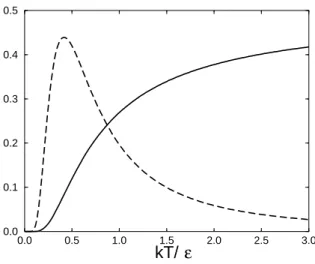
Figure 2: The energy < ǫ > and heat capacity C of a two-level system, plotted as a function of temperature. The solid curve is the mean energy divided by ǫ, u/ǫ, and the dashed curve is the heat capacity over Boltzmann’s constant, C/k.
2
The two-level system
The two-level system is pretty much the simplest system there is. It has two states: state 1 with an energy 0 and state 2 with an energy ǫ. Its partition function is defined by
Z = X
i=1,2
exp (−ǫi/kT) = 1 + exp (−ǫ/kT). (14)
Now that we know the partition function, we know the Helmholtz free energy, it is
A =−kT lnZ =−kT ln (1 + exp(−ǫ/kT)). (15) The mean energy u at a temperature T is easily found from its definition
u= X
i=1,2
piǫi =p2ǫ, (16)
as the energy of state 1 is zero and so it does not contribute to the mean energy. Now, p2 =
exp(−ǫ/kT)/Z and so
u= exp(−ǫ/kT)ǫ
1 + exp (−ǫ/kT). (17)
We can simplify this expression slightly by multiplying top and bottom of the right-hand side by exp(ǫ/kT). Then
u= ǫ
1 + exp(ǫ/kT). (18)
Now that we have the mean energy, we can calculate the heat capacity, C. This is defined by
C = ∂u ∂T (19)
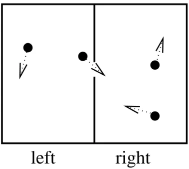
left right
Figure 3: Schematics of a box containing four molecules, all of which are moving due to their thermal kinetic energy. The box is divided in two, and there are two molecules in each half of the box, although one molecule is about to leave the left-side half and enter the right-side half.
If we take the temperature derivative of Eq. (18)
C = ǫ
2
kT2
exp(ǫ/kT)
(1 + exp(ǫ/kT))2 (20)
Both the mean energy uand the heat capacity C are plotted as functions of temperatureT in Fig. 2. The energy is zero at zero temperature; the exponential in the denominator of Eq. (18) blows up as
T →0 taking the energy to zero. At the other extreme, when the temperature is very large, then the exponential tends to one, as its argumentǫ/kT tends to zero. Then the denominator of Eq. (18) tends to two and the energy tends to ǫ/2 per system. At infinite temperature half of the systems are in the higher energy state and half are in the lower energy state. This is easy to see from the probability of being in the ground state
probability of being in state with energy 0 = 1
1 + exp(−ǫ/kT) = 1
Z. (21)
AsT tends to infinity exp(−ǫ/kT) tends to 1 andZ tends to 2. At infinite temperature the Boltzmann weights of both states are both 1, so each state is equally likely. Conversely, atT = 0, all the systems are in the ground state and so u = 0. In other words at T = 0, Z = 1 and so from Eq. (21) the probability of being in the lower energy state is 1.
3
Fluctuations and the Central Limit Theorem of Statistics
Consider a box that contains a gas of N molecules. A schematic of a box with N = 4 molecules is shown in Fig. 3. It is divided into two equal halves so the probability that a single one of these N
molecules is in the left half ispl= 1/2. The probability that it is in the right half is the same,pr = 1/2.
The entropy of a single molecule is then
S =−pllnpl−prlnpr =−(1/2) ln(1/2)−(1/2) ln(1/2) = ln 2
As the molecule has two states and they are equally likely, the entropy is just the log of the number of states, which is 2 here.
So, forN = 1 it is easy: we have a probability of 1/2 of it being in each half, thus leaving the other half empty. But oftenN is large and we want to know how many of the molecules are in each half. On average we will always getN/2 molecules in each half. But this leaves open the question: SayN = 100, what are the probabilities that say 30 or 71 or 83 of the 100 molecules are in the left-hand side of the box? We will address this question here, with the aid of the fundamental theorem in statistics: The Central Limit Theorem.
To use the Central Limit Theorem we need to introduce the idea of random numbers. A random number is simply a number whose value we don’t initially know, but we do know theprobabilitywhich with it takes each possible value. For example, the random number generators of computers typically produce a number anywhere between 0 and 1, with each possible number in that range being equally likely. Thus if ρ is a random number that will be produced by such a computer random-number generator, thenρ will be any number between 0 and 1, with equal probability of being any number in that range. Another example would be if the random numberρis the outcome of the throw of a dice. Then ρ would be one of 1, 2, 3, 4, 5 or 6, with each of the 6 numbers being equally likely.
For the case of the gas of molecules we define a random number ρi for the ith molecule that is
equal to 1 if the molecule is in the left-hand half and equal to 0 if the molecule is in the right-hand half. The ith molecule is one of the N, so i= 1, 2, 3, 4,. . ., N. Also note that the mean value of ρi,
denoted by hρii, equals one half because on average half the ρi are 1, and the other half are zero. So, hρii= 1/2.
With this definition of ρi, the total number of molecules in the left-hand half is the sum over the
ρi
number on left-hand side of the box =Sl = N
X
i=1
ρi
because for each molecule that is on the left,ρi = 1.
First let us consider the average of Sl, hSli. This is
hSli=h N X i=1 ρii= N X i=1 hρii= N X i=1 1 2 = N 2
Now the Central Limit Theorem (CLT) is a theorem for sums over random numbers. It concerns the variations or fluctuations of a sum, in this caseSl, about its mean valuehSli. The point is that the
sum of a set of random numbers is itself a random number, and if we know the probabilities with which the individual random numbers take particular values, then the CLT tells us about the probabilities with which the sum takes particular values. So, here Sl is itself a random number and the CLT tells
about how broad the distribution of possible values of Sl is.
In fact it clarifies things if we subtract off the mean value of Sl, to get a new random number R
defined by
Note that by its definition the average or mean value of R must be zero. Then R is the random fluctuation or variation of the the sumSlfrom its average value. ForSl, the CLT states that, for large
values of N, the root-mean-square of R is given by
hR2
i ≃N or hR2
i1/2
≃N1/2
The crucial feature (which you must remember) is that the root-mean-square of R, i.e., the standard deviation of Sl about its mean value, scales as the square root of N, while hSli itself scales linearly
with N.
Thus, for N = 100 molecules in the box, the number in the left-hand side at any instant will typically be somewhere in the range 50−1001/2
to 50 + 1001/2
, i.e., from 40 to 60. At any given instant it is unlikely that there will be exactly 50 molecules in one half, but it is very likely that that there will be between 40 and 60 molecules. This corresponds to a fraction on the left of between 0.4 and 0.6.
However, if there areN = 106
molecules in the box then in one half there will be between 500,000-1,000 and 500,000+500,000-1,000, i.e., between 499,999 and 50500,000-1,000 molecules on the left. This corresponds to a fraction on the left in the range 0.499 to 0.501. We see that for N = 106
we have very close to half the molecules in each half at all times. ForN = 1023
- a reasonable value for a volume of around 1 litre - the fraction in one half lies in the range 0.5−(1023
)1/2
to 0.5 + (1023
)1/2
, which is 0.49999999999999 to 0.50000000000001. Here we have essentially exactly half the molecules in each half of the box at all times.
The CLT is used in pretty much all of statistics. As an example, consider opinion polling. Pollsters typically poll a few thousand people, in order to use the CLT and get reliable results. For example, say they are interested in knowing what percentage of people will vote Conservative or Labour. Let us assume that in fact a fraction 0.54 will vote Conservative and 0.46 will vote Labour. If they ask 100 people then the number that will say they will vote Labour will be in the range 46 −1001/2
to 46 + 1001/2
, i.e., from 36 to 56. Thus the pollsters could find that anywhere between 36% and 56% would vote Labour and between 44% and 64% would vote Conservative. These estimates are not accurate enough to tell whether the Conservatives or Labour are more popular. However, if they asked 1000 people then between 460−10001/2
and 460 + 10001/2
, i.e., from 428 to 492 would vote Labour. This gives a % voting Labour somewhere between 43% and 49%, and a % voting Conservative of 51% to 57%. Thus, a poll of 1000 people will reliably show that the Conservatives are more popular while a poll of 100 will not. This is why Mori etc poll large numbers of people.
4
States with different numbers of particles
So far we have dealt with states that only differ in their energies, i.e., state 1 has energy ǫ1, state
2 has energy ǫ2 6= ǫ1, etc. Here, we will consider states that also have varying numbers of particles,
i.e., state 1 has energy ǫ1 and a number of particles n1, state 2 has energy ǫ2 6=ǫ1 and a number of
particles n2 6=n1, etc. Dealing with states with different numbers of particles is completely analogous
to dealing with states with different energies. So we won’t derive any expressions, we will just write them down. See any of the recommended textbooks for derivations.
So, recall that for states that differ only by their energy the probability of being in a state i with an energyǫi is pi(ǫi)∝exp(−ǫi/kT) pi(ǫi) = exp(−ǫi/kT) Z for Z = X i exp(−ǫi/kT)
When the number of particles varies as well the probability also depends on the number of particles. We denote the number of particles in state i, as ni. Then the probability of state i is p(ǫi, ni). The
dependence of the probability on ni is exponential, just as its dependence on ǫi. The coefficient in
the exponential is µ/kT, where µ is the chemical potential. Just as the temperature T controls the probabilities of states with different energies, the chemical potential µ controls the probabilities of states with different numbers of particles. So we have
pi(ǫi, ni)∝exp(−ǫi/kT +niµ/kT) pi(ǫi, ni) = exp(−ǫi/kT +niµ/kT) Ξ and with Ξ =X i exp(−ǫi/kT +niµ/kT)
where Ξ is the partition function when the number of particles can vary as well as the energy. Ξ is the sum over all possible states of the system, just as Z is, but now each state contributes a factor that depends on ni as well as ǫi. The probability of a state is proportional to exp(µ×number of particles
in state/kT) and so if the chemical potential µ is increased, states with large numbers of particles in them become more probable, more likely. Also, unlike the temperature, the chemical potential can in general be either positive or negative. If it is positive, states with large numbers of particles are favoured, whereas if it is negative, states with small numbers of particles are favoured.
As an example, consider a system that has just two states: state one with 0 particles, n1 = 0, and
0 energy,ǫ1 = 0, and state two with 1 particle, n2 = 1, and energy ǫ2/kT = 1, i.e., the energy is 1 in
units of kT. The chemical potential µ/kT = 2, i.e., is 2 in units of kT. To calculate the probabilities of being in each of the states,p1 and p2, we first need to calculate the partition function
Ξ =
2
X
i=1
exp(−ǫi/kT +niµ/kT) = exp(−0 + 0×2) + exp(−1 + 1×2) = 1 + e = 3.72
Then the probabilities are
pi = exp(−ǫi/kT +niµ/kT) Ξ p1 = exp(0) 3.72 = 0.269 p2 = exp(1) 3.72 = 0.731 the state with the particle in it is about three times as probable as the state without.
5
Fermi-Dirac and Bose-Einstein Statistics
Now we will do statistical mechanics on particles that behave quantum mechanically. Of course, quantum-mechanical particles come in two varieties: fermions and bosons. Particles with half integral spin, electrons, 3
He etc., are fermions and particles with zero or integral spin, photons, 4
He etc., are bosons. The crucial difference between fermions and bosons is that fermions obey Pauli’s exclusion principle which states that no more than one fermion can occupy an energy level. An energy level can be empty, i.e., containing 0 fermions, or it can contain 1 fermion, no more. An energy level can contain any number of bosons, indeed very cold 4
He undergoes what is known as Bose-Einstein condensation and then a significant fraction of all the atoms (there could be 1023
atoms) in the helium are all in one level.
5.1
A single level with Fermi-Dirac statistics
Consider a single energy level (don’t worry about where this level comes from for now) with an energy
ǫ. This level can accommodate a fermion (no more than one of course). This level has two states: state 1 without a fermion in it, energy = 0, and state 2 with a fermion, energy = ǫ. Thus ǫ1 = 0,
n1 = 0, and ǫ2 = ǫ, n2 = 1. We want to work at fixed chemical potential µ and temperature
T. Then the appropriate weight of a state i with energy ǫi = niǫ and number of particles ni is
exp[−niǫ/kT +niµ/kT].
The canonical partition function Ξ is just the sum of these weights over the two possible states, i.e.,
Ξ = exp [−n1ǫ/kT +n1µ/kT] + exp [−n2ǫ/kT +n2µ/kT], (22)
or
Ξ = 1 + exp[(µ−ǫ)/kT]. (23) Now that we have the partition function we can calculate the probabilities of being in the each of the two states, p1 and p2,
p1 = 1 Ξ = 1 1 + exp[(µ−ǫ)/kT] p2 = exp[(µ−ǫ)/kT] Ξ = exp(µ−ǫ)/kT] 1 + exp[(µ−ǫ)/kT]
We can also work out the average number of fermions in the energy level, n. It is just a sum over the two states, with each state contributing the probability of it being occupied times the number of fermions in it. For our system with two states
n=p1n1+p2n2 = 0 +
exp[(µ−ǫ)/kT]
1 + exp[(µ−ǫ)/kT]×1 =
1
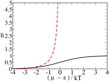
exp[(ǫ−µ)/kT] + 1. (24) Because no more than one fermion can occupy the level n can never be more than 1. In Eq. (24) the exponential is never negative so n equals 1, divided by 1 plus a nonnegative quantity, and so lies between 0 and 1. A plot of n as a function of µ−ǫ is shown in Fig. 4.
5.2
A single level with Bose-Einstein statistics
Again consider a single energy level with an energy ǫ. This level now accommodates bosons, any number of them. The level has an infinite number of states: one without a boson in it, energy= 0; one with 1 boson, energy ǫ; one with 2 bosons, energy 2ǫ; one with 3 bosons, energy 3ǫ; etc. Again we want to work at fixed chemical potential µ and temperatureT. Then the appropriate weight of a state with energy nǫand number of particles n is exp[−nǫ/kT +nµ/kT]. The partition function Ξ is just the sum of these weights over all possible states. So,
Ξ = 1 + exp[(µ−ǫ)/kT] + exp[2(µ−ǫ)/kT] + exp[3(µ−ǫ)/kT] +· · ·
Ξ = 1 + exp[(µ−ǫ)/kT] + (exp[(µ−ǫ)/kT])2+ (exp[(µ−ǫ)/kT])3+· · · (25) because for anyx, exp(2x) = [exp(x)]2
etc. Here the 1st term is for an empty level, the 2nd for a level with 1 boson, the 3rd for two bosons in the level, etc. If we define y= exp[(µ−ǫ)/kT], then we have
Ξ = 1 +y+y2 +y3 +· · · yΞ = y+y2+y3+y4+· · · Ξ−yΞ = 1 Ξ = 1 1−y, (26)
-4
-3
-2
-1
0
1
2
3
4
( µ − ε ) /
0
0.5
1
1.5
2
2.5
3
3.5
4
4.5
5
n
kT
Figure 4: Plots of the mean number of particles, n, in a single energy level of energy ǫ, as a function of the chemical potential minus this energy, over kT. The solid black curve is for fermions and the dashed grey curve is for bosons. Note that the curve for bosons diverges at µ=ǫ and is not defined for µ > ǫ.
and
Ξ = 1
1−exp[(µ−ǫ)/kT]. (27) The probability of the state with n bosons in it is then just
pn= exp [n(µ−ǫ)/kT] Ξ so p0 = 1 Ξ p1 = exp [(µ−ǫ)/kT] Ξ · · ·
We can also work out the average number of bosons in the level, n. It is just a sum over each state, with each state contributingpn×n. So,
n = p0×0 +p1×1 +p2×2 +· · · n = 0 + exp [(µ−ǫ)/kT] Ξ ×1 + exp [2(µ−ǫ)/kT] Ξ ×2 + exp [3(µ−ǫ)/kT] Ξ ×3 +· · · n = y+ 2y 2 + 3y3 +· · · Ξ (28)
The sum on top isy+ 2y2
+ 3y3
+· · ·. Now, if we take the derivative of Ξ = 1 +y+y2
+y3 +· · ·we have dΞ dy = 1 + 2y+ 3y 2 +· · ·
and then if we multiply by y
ydΞ
dy =y+ 2y
2
+ 3y3 +· · ·
which is the sum we need. So the top half of the expression for n is equal to ydΞ/dy. As we know Ξ = 1/(1−y) this derivative is easy to calculate
dΞ dy =
d(1−y)−1
dy = (1−y)
and ydΞ dy =y(1−y) −2 so n= y+ 2y 2 + 3y3 +· · · Ξ = y(1−y)−2 (1−y)−1 =y(1−y) −1 = exp [(µ−ǫ)/kT] 1−exp[(µ−ǫ)/kT] and finally n= 1 exp[(ǫ−µ)/kT]−1
Because many bosons can occupy the level n ranges from 0 to∞. n =∞ when exp[(ǫ−µ)/kT] = 1. i.e., whenǫ=µ. Note thatµcannot be larger thanǫ, if it were larger than ǫ, exp[(ǫ−µ)/kT]<1 and
n would be negative. n is an average number of particles in a level, it must be nonnegative, you can’t have a minus number of particles. Ifµis increased so that it equalsǫ then Bose-Einstein condensation takes place. This phenomenon is beyond the scope of this course. Here we will only consider the case
ǫ−µ >0. A plot of n as a function of µ−ǫ is shown in Fig. 4.
6
Averages and the relationship between the partition
func-tion and thermodynamic quantities
6.1
Averages
The average of a quantity x is denoted byhxi. By definition it is given by
hxi=X
i
pixi, (29)
where the sum is over all possible states, and xi is the value of the quantity x in state i. This works
for any quantity that has a definite value in a given state. Here pi is the probability that the system
is in statei. Thus, if we can calculate the value of x in each state and can find the probabilitiespi we
can find the average value of x.
The above expression is always true, but for the rest of this section we will consider only averages at constant T.
6.2
Average quantities at constant
T
We have already found that the probability pi that a system is in a state i with an energy ǫi is
pi = exp(−ǫi/kT)/Z, where Z is the partition function
Z =X
i
exp(−ǫi/kT)
Knowing the probabilitiespi, we can calculate averages: the average of x is
hxi=X i pixi = 1 Z X i xiexp(−ǫi/kT),
For example, when x is the energy ǫ, we have an expression for the average energy hǫi. This is given by just the above equation with xreplaced by ǫ
hǫi= 1
Z
X
i
ǫiexp(−ǫi/kT).
For example, for a simple system with only 2 states. State 1 with energy ǫ1 and state 2 with energy
ǫ2 we have that the partition functionZ is
Z = exp(−ǫ1/kT) + exp(−ǫ2/kT)
and the average energy is
hǫi= 1
Z [ǫ1exp(−ǫ1/kT) +ǫ2exp(−ǫ2/kT)] =
ǫ1exp(−ǫ1/kT) +ǫ2exp(−ǫ2/kT)
exp(−ǫ1/kT) + exp(−ǫ2/kT)
.
6.2.1 The partition function Z and the Helmholtz free energy A
Here we will relate the statistical-physics quantity, Z, and the thermodynamics quantity, A, the Helmholtz free energy. Recall from your thermodynamics lectures that the Helmholtz free energy is defined by
A=U −kT S
whereU is the thermodynamic energy. Note thatSwas given in different units in your thermodynamics course so in that course there was no factor of k in this equation.
Earlier, we found that the typical size of fluctuations about the mean was equal to the mean itself divided by N1/2
. Thus for macroscopic systems (N ≃ 1022
or more, which is what thermodynamics considers) these fluctuations are only a fraction 10−11
of the mean and so are negligible. Thus the energy is always indistinguishable from the average, hǫi, so,
U =hǫi
This is the, trivial, relationship between the average energy in statistical physics and the thermody-namic energy.
To see how we can calculate the Helmholtz free energy in statistical physics we will start from Shannon’s equation for the entropy. This is
S =−X i pilnpi =− 1 Z X i exp(−ǫi/kT) ln exp(−ǫi/kT) Z =−1 Z X i exp(−ǫi/kT) h − ǫi kT −lnZ i
where we usedpi = exp(−βǫi)/Z. We can simplify the above expression
S = 1 ZkT X i exp(−ǫi/kT)ǫi+ lnZ Z X i exp(−ǫi/kT) S = hǫi kT + lnZ
because the first sum over Z is simply the definition of the average energy hǫi (over kT), and the second sum is justZ. At the moment the last equation just relates the entropy S, the average energy
hǫi and the log of the partition function. But if we take the thermodynamic equation A = U −kT S
and rearrange it we have
S = U
kT − A kT.
If we compare this equation with the one above, clearly
A=−kTlnZ.
So, from this equation if we can calculate the partition function Z, then we can find the Helmholtz free energy A simply by taking its logarithm and multiplying it by−kT.
Finally, we note that if we take the derivative of the partition function Z with respect to temper-ature, we obtain ∂Z ∂T = X i ∂ ∂T exp (−ǫi/kT) = 1 kT2 X i ǫiexp (−ǫi/kT) = hǫiZ kT2. or 1 Z ∂Z ∂T = hǫi kT2 But ∂lnZ ∂T = 1 Z ∂Z ∂T so ∂lnZ ∂T = hǫi kT2 or hǫi=kT 2∂lnZ ∂T
So, we can calculate the average energy by calculatingZand then taking the derivative of its logarithm.
7
Classical Statistical Mechanics
So far we have defined the partition functionZas a sum over all the states, with each state contributing its Boltzmann weight,
Z =X
i
exp (−ǫi/kT). (30)
But we would now like to consider classical systems such as gases at relatively high temperatures. There the state is specified by specifying the positions and velocities (or equivalently the momenta) of all the particles. These positions and velocities arecontinuous variables, i.e., they are notquantised and can therefore take any value, not just a discrete set of values. By gases at relatively high temperatures we mean gases where quantum mechanical effects are small and so we can treat them as being composed of particles which can be treated using classical mechanics. This is true of the atmosphere, but not of low temperature helium. In low temperature helium we need to take quantum mechanics into account. A gas has a very large number of molecules moving in three dimensions but to keep things simple we will just consider a single particle moving in one dimension. The generalisation to many particles is easy. So consider a single particle in a one-dimensional box so that it can only move back and fore along the x axis. The microscopic state of the system of one particle is specified by specifying the x
coordinate of the particle and the x-component of the momentum of the particle, px. So, if we take
one microscopic configuration specified by x and px, and move the particle from x to x+ dx then we
have a new microscopic state. We can also generate a new configuration by changing the momentum frompx topx+ dpx. So, in order to sum over all the states we must integrate over all possible positions
and momenta of the particle. The sum becomes an integral
X
→
Z
dxdpx. (31)
Also, the energy ǫi, which did depend on the state i, hence the subscript i on ǫ, is now a function of
x and p: ǫ(x, p). Putting all this together,
Z ∝
Z
exp(−ǫ(x, p)/kT)dxdpx. (32)
The proportional sign, ∝, is there because we expect the partition function to be dimensionless as it is a sum of pure numbers, the Boltzmann weights. This is clear from Eq. (30). The integral on the right hand side of Eq. (32) has dimensions of length times momentum (from the factor dxdpx). So,
we need a proportionality constant with dimensions of one over length times momentum to put on the right hand side of Eq. (32). In fact, the correct proportionality constant is one over Planck’s constant, which has the correct dimensions. So,
Z =h−1
Z
exp(−ǫ(x, p)/kT)dxdpx (33)
I am not going to prove this. It is also not very important as changing the proportionality constant does not actually change properties we can measure such as the heat capacity etc. Indeed in the very next section I am going to drop the constant in front of the integral. The important thing to remember is that in classical systems you just replace thesums over states byintegrals over all possible values of the variables like position and momentum.
7.1
Example
For example, consider a particle restricted to a box of length L, stretching from x = 0 to x=L, and a momentum range from px = 0 to px =m. If the energy is zero inside the box and infinite inside it
the classical partition function is
Z = h−1 Z dxexp(−ǫ(x, p)/kT)dxdpx =h −1 Z x=L x=0 dx Z px=m px=0 dpxexp(0) = h−1 [x]x=L x=0 ×[px]p x=m px=0 =h −1 ×L×m= Lm h
Compare this with the partition function Z for a quantum mechanical system with Ω states all with zero energy Z = Ω X i=1 exp (−0/kT) = Ω
Note that for the quantum mechanical partition function doubling the number of states doubles the partition function while the classical partition function doubles if either the length or the momentum range are doubled. Essentially, the longer the length of the box the more possible positions of the particle there are and this is equivalent to increasing the number of possible states.
7.2
The equipartition theorem
This theorem applies to classical systems in which the energy varies quadratically with a coordinate, i.e., the energy varies as some constant times the square of the coordinate. It does not matter what the coordinate is. For example, in an ideal gas there is a kinetic energy of (p2
x +p
2
y +p
2
z)/(2m) per
particle which is quadratic. Also, the energy of a Hookean spring, = (1/2)kx2
, is quadratic. We can derive the theorem using any quadratic energy.
For example, consider the quadratic energy
ǫ(p) =bp2
, (34)
whereb is a constant. If pis the momentum of a particle along say the xaxis, thenb would be 1/2m, where m is the mass of the particle.
The partition function for the coordinate pis obtained by integrating over all possible values of p.
Z =
Z ∞ −∞
dpexp(−bp2
/kT), (35)
We have dropped the factor ofh−1
as it is a constant and will not affect the energy, which is a derivative of the logarithm of the partition function. The integral is a simple Gaussian integral like
Z ∞ −∞ exp(−az2 )dz=π a 1/2 . (36) So, Z = πkT b 1/2 , (37)
the quadratic energy has contributed a factor which is proportional to T1/2
to the partition function. This is always true of any coordinate which has a contribution to the energy which depends on the square of the coordinate.
We would like the average energy U =hǫi, which is obtained from the derivative of the partition function (see previous section)
U = kT2∂lnZ ∂T =kT 2 ∂ ∂T ln πkT b 1/2 = 1 2kT 2 ∂ ∂T ln πkT b = 1 2kT 2 ∂ ∂T lnT + ln πk b = 1 2kT 2 1 T + 0 = 1 2kT (38) The average energy U of a particle with an energy which depends quadratically on its momentum is just (1/2)kT. Note that it does not depend on the value of b, changing b has no effect on the mean energy hǫi. This is general for any quadratic term, and is called the equipartition theorem
Equipartition theorem = For aclassicalsystem anyquadraticterm in the energy contributes (1/2)kT to the energy.
For example, in an classical gas, each of the N particles has a kinetic energy (p2
x+p
2
y +p
2
z)/2m —
three quadratic terms, one each from the x, y and z directions — therefore each gas particle has an energy (3/2)kT and N particles have an energy (3/2)N kT.
The heat capacity is obtained from
C = ∂U
∂T
= 1
2k. (39)
The quadratic term has contributed k/2 to the heat capacity C; this is a general result. The heat capacity C = (1/2)k × the number of quadratic terms in the energy.
7.3
When is a gas classical and when are quantum mechanical effects
important
We would like to know when we can treat the molecules in a gas using classical mechanics and when quantum mechanics is required. For example, the above simple treatment of a gas is only valid, only gives the right answer, when the molecules can be treated using classical mechanics. So to reassure ourselves that our answer is right, we would like to satisfy ourself that classical mechanics is a valid description of the gas molecules.
Now, classical mechanics of course treats molecules as point-like particles with a definite position, whereas within quantum mechanics (QM) we have the wave/particle duality. In QM we have Heisen-berg’s uncertainty principle which states that ∆x∆p≈~, where ∆x is the uncertainty or blurring of
the position x, and ∆p is the uncertainty in momentum p. Now, if the typical separation between the molecules in a gas, call it s, is much larger than the blurring of the positions of the molecules due to QM, ∆x, then this blurring can be neglected and classical mechanics is a good approximation. However, ifs <∆x then the uncertainty in the position of the particles is greater than their distance apart, i.e., their wavefunctions are overlapping. Then classical mechanics is not a good approximation, we have to use QM and calculate the wavefunction etc.
We estimate the uncertainty in x by finding the uncertainty inp, ∆p, and then using Heisenberg’s uncertainty principle: ∆x = ~/∆p. To find ∆p, we start with the equipartition theorem. If a gas
is classical then the average kinetic energy of a particle for motion along one of the axes, x, y or z, is simply (1/2)kT. This average kinetic energy is just hp2
i/2m, where hp2
i is just the average of the square of the momentum along thex axis, p. So, we have
mean K.E. = hp 2 i 2m = 1 2kT hp 2 i=mkT. (40) and p hp2i= (mkT)1/2 (41)
So the root-mean-square momentum php2i = (mkT)1/2
. This gives the typical magnitude of the momentum and this momentum can be in either direction so the uncertainty in the momentum is approximately the same as this magnitude ∆p≈p
hp2i= (mkT)1/2
. Combining this with Heisenberg’s uncertainty principle we have
∆x≈ ~
∆p ≈
~
(mkT)1/2 (42)
This uncertainty in,x, ∆x is often called the thermal or de Broglie wavelength.
For a classical-mechanics description of a gas to be valid ∆x must be smaller than s. Now, if the gas is at a density ofρmolecules per cubic metre, then the volume per molecule is 1/ρ. The separation
s is roughly the cube root of the volume per particle sos≈(1/ρ)1/3
. So finally, for a gas of molecules to be classical we require that
∆x≪s ~
(mkT)1/2 ≪ 1
ρ1/3 (43)
Let us put some numbers into this equation. Atmospheric pressure is about p= 105
Pa, and p=ρkT. This means that at room temperature, kT = 4×10⁻²¹
J, ρ = 105
/(4×10−21
) ≈ 1026
molecules/m3
. So the average distance between molecules s ≈ (1/1026
)1/3
≈ 10−9
m or about 1nm. Now for the QM uncertainty in the position of the molecule, ∆x, at room temperature. The mass of a proton is 1.7×10⁻²⁷
kg and the most abundant gas in the atmosphere is 14
N2 which has a mass 2×14×1.7×
10−27 ≈ 10−26 kg. Thus ∆x≈ ~/(mkT)≈ 10−34 /(10−26 ×4×10−21 )1/2 ≈10−10 m. So the blurring of the position of the nitrogen molecules due to QM effects, at room temperature, is about 0.1nm, or 1 tenth of their average spacing in Earth’s atmosphere. Therefore classical mechanics works for the gas molecules in the atmosphere.