THESIS FOR THE DEGREE OF DOCTOR OF PHILOSOPHY
Analysis, Modeling and Control of Doubly-Fed
Induction Generators for Wind Turbines
ANDREAS PETERSSON
Division of Electric Power Engineering Department of Energy and Environment CHALMERS UNIVERSITY OF TECHNOLOGY
Analysis, Modeling and Control of Doubly-Fed Induction Generators for Wind Turbines
ANDREAS PETERSSON ISBN 91-7291-600-1
c
ANDREAS PETERSSON, 2005.
Doktorsavhandlingar vid Chalmers tekniska h¨ogskola Ny serie nr. 2282
ISSN 0346-718x
Division of Electric Power Engineering Department of Energy and Environment Chalmers University of Technology SE-412 96 G¨oteborg
Sweden
Telephone + 46 (0)31-772 1000
Chalmers Bibliotek, Reproservice G¨oteborg, Sweden 2005
Analysis, Modeling and Control of Doubly-Fed Induction Generators for Wind Turbines ANDREAS PETERSSON
Division of Electric Power Engineering Department of Energy and Environment Chalmers University of Technology
Abstract
This thesis deals with the analysis, modeling, and control of the doubly-fed induction gener-ator (DFIG) for wind turbines. Different rotor current control methods are investigated with the objective of eliminating the influence of the back electromotive force (EMF), which is that of, in control terminology, a load disturbance, on the rotor current. It is found that the method that utilizes both feed forward of the back EMF and so-called “active resistance” manages best to suppress the influence of the back EMF on the rotor current, particularly when voltage sags occur, of the investigated methods. This method also has the best stability properties. In addition it is found that this method also has the best robustness to parameter deviations.
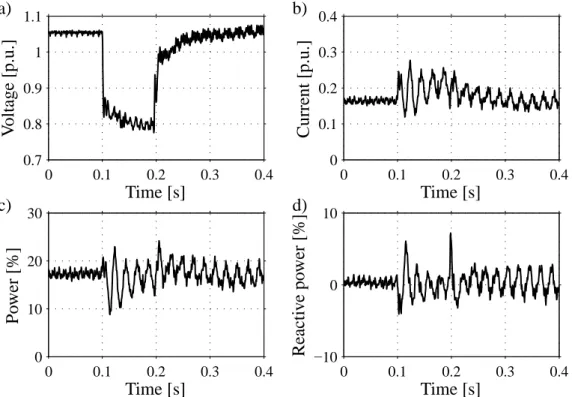
The response of the DFIG wind turbine system to grid disturbances is simulated and ver-ified experimentally. A voltage sag to 80% (80% remaining voltage) is handled very well. Moreover, a second-order model for prediction of the response of small voltage sags of the DFIG wind turbines is derived, and its simulated performance is successfully verified exper-imentally.
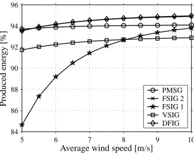
The energy production of the DFIG wind turbine is investigated and compared to that of other wind turbine systems. The result found is that the energy capture of the DFIG wind tur-bine is almost the same as for an active stall-controlled fixed-speed (using two fixed speeds) wind turbine. Compared to a full-power-converter wind turbine the DFIG wind turbine can deliver a couple of percentage units more energy to the grid.
Voltage sag ride-through capabilities of some different variable-speed wind turbines has been investigated. It has been found that the energy production cost of the investigated wind turbines with voltage sag ride-through capabilities is between 1–3 percentage units higher than that of the ordinary DFIG wind turbine without the ride-through capability.
Finally, a flicker reduction control law for stall-controlled wind turbines with induction generators, using variable rotor resistance, is derived. The finding is that it is possible to reduce the flicker contribution by utilizing the derived rotor resistance control law with 40– 80% depending on the operating condition.
Keywords: Doubly-fed induction generator, wind turbine, wind energy, current control, voltage sag, power quality.
Acknowledgements
This research project has been carried out at the Department of Energy and Environment (and the former Department of Electric Power Engineering) at Chalmers University of Tech-nology. The financial support provided by the Swedish National Energy Agency is gratefully acknowledged.
I would like to thank my supervisors Dr. Torbj¨orn Thiringer and Prof. Lennart Harnefors for help, inspiration, and encouragement. I would also like to thank my examiner Prof. Tore Undeland for valuable comments and encouragement. Thanks goes to my fellow Ph.D. stu-dents who have assisted me: Stefan Lundberg for a pleasant collaboration with the efficiency calculations, Dr. Rolf Ottersten for many interesting discussions and a nice cooperation, es-pecially with the analysis of the full-power converter, Dr. Tom´aˇs Petr˚u for valuable and time saving collaboration with practical field measurement set-ups, and Oskar Wallmark for a good companionship and valuable discussions.
Many thanks go to the colleagues at the Division of Electric Power Engineering and the former Department of Electric Power Engineering, who have assisted me during the work of this Ph.D. thesis.
Table of Contents
Abstract iii
Acknowledgements v
Table of Contents vii
1 Introduction 1
1.1 Review of Related Research . . . 2
1.2 Purpose and Contributions . . . 4
1.3 List of Publications . . . 5
2 Wind Energy Systems 7 2.1 Wind Energy Conversion . . . 7
2.1.1 Wind Distribution . . . 7
2.1.2 Aerodynamic Power Control . . . 8
2.1.3 Aerodynamic Conversion . . . 8
2.2 Wind Turbine Systems . . . 9
2.2.1 Fixed-Speed Wind Turbine . . . 11
2.2.2 Variable-Speed Wind Turbine . . . 11
2.2.3 Variable-Speed Wind Turbine with Doubly-Fed Induction Generator 12 2.3 Doubly-Fed Induction Generator Systems for Wind Turbines . . . 13
2.3.1 Equivalent Circuit of the Doubly-Fed Induction Generator . . . 14
2.3.2 Power Flow . . . 16
2.3.3 Stator-to-Rotor Turns Ratio . . . 17
2.3.4 Lowering Magnetizing Losses . . . 18
2.3.5 Other Types of Doubly-Fed Machines . . . 19
3 Energy Efficiency of Wind Turbines 23 3.1 Determination of Power Losses . . . 23
3.1.1 Aerodynamic Losses . . . 23
3.1.2 Gearbox Losses . . . 24
3.1.3 Induction Generator Losses . . . 24
3.1.4 Converter Losses . . . 26
3.1.5 Total Losses . . . 28
3.2 Energy Production of the DFIG System . . . 29
3.2.1 Investigation of the Influence of the Converter’s Size on the Energy Production . . . 29
3.2.2 Reduction of Magnetizing Losses . . . 31
3.3 Comparison to Other Wind Turbine Systems . . . 31
3.4 Discussion . . . 33
3.5 Conclusion . . . 34
4 Control of Doubly-Fed Induction Generator System 35 4.1 Introduction . . . 35
4.1.1 Space Vectors . . . 35
4.1.2 Power and Reactive Power in Terms of Space Vectors . . . 36
4.1.3 Phase-Locked Loop (PLL)-Type Estimator . . . 36
4.1.4 Internal Model Control (IMC) . . . 37
4.1.5 “Active Damping” . . . 38
4.1.6 Saturation and Integration Anti-Windup . . . 40
4.1.7 Discretization . . . 40
4.2 Mathematical Models of the DFIG System . . . 41
4.2.1 Machine Model . . . 41 4.2.2 Grid-Filter Model . . . 43 4.2.3 DC-Link Model . . . 44 4.2.4 Summary . . . 45 4.3 Field Orientation . . . 45 4.3.1 Stator-Flux Orientation . . . 45 4.3.2 Grid-Flux Orientation . . . 46
4.4 Control of Machine-Side Converter . . . 47
4.4.1 Current Control . . . 47
4.4.2 Torque Control . . . 50
4.4.3 Speed Control . . . 50
4.4.4 Reactive Power Control . . . 52
4.4.5 Sensorless Operation . . . 54
4.5 Control of Grid-Side Converter . . . 55
4.5.1 Current Control of Grid Filter . . . 56
4.5.2 DC-Link Voltage Control . . . 56
5 Evaluation of the Current Control of Doubly-Fed Induction Generators 59 5.1 Stability Analysis . . . 59
5.1.1 Stator-Flux-Oriented System . . . 59
5.1.2 Grid-Flux-Oriented System . . . 64
5.1.3 Conclusion . . . 66
5.2 Influence of Erroneous Parameters on Stability . . . 66
5.2.1 Leakage Inductance,Lσ . . . 67
5.2.2 Stator and Rotor Resistances,RsandRR . . . 67
5.3 Experimental Evaluation . . . 70
5.3.1 Comparison Between Stator-Flux and Grid-Flux-Oriented System . 71 5.4 Impact of Stator Voltage Sags on the Current Control Loop . . . 71
5.4.1 Influence of Erroneous Parameters . . . 73
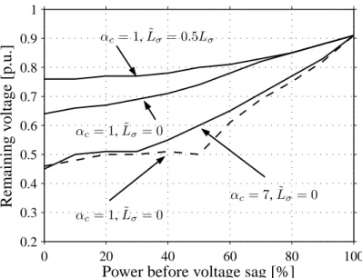
5.4.2 Generation Capability During Voltage Sags . . . 74
5.5 Flux Damping . . . 74
5.5.2 Grid-Flux Orientation . . . 76
5.5.3 Parameter Selection . . . 76
5.5.4 Evaluation . . . 77
5.5.5 Response to Symmetrical Voltage Sags . . . 77
5.6 Conclusion . . . 79
6 Evaluation of Doubly-Fed Induction Generator Systems 81 6.1 Reduced-Order Model . . . 81
6.2 Discretization of the Doubly-Fed Induction Generator . . . 81
6.2.1 Stator-Flux Orientation . . . 82
6.2.2 Grid-Flux Orientation . . . 82
6.3 Response to Grid Disturbances . . . 83
6.4 Implementation in Grid Simulation Programs . . . 87
6.5 Summary . . . 88
7 Voltage Sag Ride-Through of Variable-Speed Wind Turbines 89 7.1 Voltage Sags . . . 90
7.1.1 Symmetrical Voltage Sags . . . 90
7.1.2 Unsymmetrical Voltage Sags . . . 90
7.2 Full-Power Converter . . . 92
7.2.1 Analysis . . . 92
7.2.2 Discussion . . . 98
7.2.3 Evaluation . . . 99
7.2.4 Conclusion . . . 100
7.3 Doubly-Fed Induction Generator with Shunt Converter . . . 102
7.3.1 Response to Small Voltage Sags . . . 103
7.3.2 Response to Large Voltage Sags . . . 110
7.3.3 Candidate Ride-Through System . . . 111
7.3.4 Evaluation of the Ride-Through System . . . 114
7.4 Doubly-Fed Induction Generator with Series Converter . . . 118
7.4.1 Possible System Configurations . . . 118
7.4.2 System Modeling . . . 120
7.4.3 Control . . . 123
7.4.4 Speed Control Operation . . . 125
7.4.5 Response to Voltage Sags . . . 126
7.4.6 Steady-State Performance . . . 127
7.4.7 Discussion and Conclusion . . . 131
7.5 Conclusion . . . 132
8 Flicker Reduction of Stalled-Controlled Wind Turbines using Variable Rotor Resistances 133 8.1 Modeling . . . 133
8.1.1 Reduced-Order Model . . . 134
8.2 Current Control . . . 135
8.2.1 Evaluation . . . 138
8.3 Reference Value Selection . . . 139
8.4 Evaluation . . . 141 8.4.1 Flicker Contribution . . . 143 8.4.2 Flicker Reduction . . . 144 8.5 Conclusion . . . 145 9 Conclusion 147 9.1 Future Research . . . 148 References 149 A Nomenclature 159 B Data and Experimental Setup 163 B.1 Data of the DFIG . . . 163
B.2 Laboratory Setup . . . 164
B.2.1 Data of the Induction Generator . . . 164
Chapter 1
Introduction
The Swedish Parliament adopted new energy guidelines in 1997 following the trend of mov-ing towards an ecologically sustainable society. The energy policy decision states that the objective is to facilitate a change to an ecologically sustainable energy production system. The decision also confirmed that the 1980 and 1991 guidelines still apply, i.e., that the nu-clear power production is to be phased out at a slow rate so that the need for electrical energy can be met without risking employment and welfare. The first nuclear reactor of Barseb¨ack was shut down 30th of November 1999. Nuclear power production shall be replaced by im-proving the efficiency of electricity use, conversion to renewable forms of energy and other environmentally acceptable electricity production technologies [97]. According to [97] wind power can contribute to fulfilling several of the national environmental quality objectives de-cided by Parliament in 1991. Continued expansion of wind power is therefore of strategic importance. The Swedish National Energy Agency suggest that the planning objectives for the expansion of wind power should be 10 TWh/year within the next 10–15 years [97]. In Sweden, by the end of 2004, there was 442 MW of installed wind power, corresponding to 1% of the total installed electric power in the Swedish grid [23, 98]. These wind turbines produced 0.8 TWh of electrical energy in 2004, corresponding to approximately 0.5% of the total generated and imported electrical energy [23, 98].
Wind turbines (WTs) can either operate at fixed speed or variable speed. For a fixed-speed wind turbine the generator is directly connected to the electrical grid. For a variable-speed wind turbine the generator is controlled by power electronic equipment. There are several reasons for using variable-speed operation of wind turbines; among those are pos-sibilities to reduce stresses of the mechanical structure, acoustic noise reduction and the possibility to control active and reactive power [11]. Most of the major wind turbine man-ufactures are developing new larger wind turbines in the 3-to-5-MW range [3]. These large wind turbines are all based on variable-speed operation with pitch control using a direct-driven synchronous generator (without gearbox) or a doubly-fed induction generator (DFIG). Fixed-speed induction generators with stall control are regarded as unfeasible [3] for these large wind turbines. Today, doubly-fed induction generators are commonly used by the wind turbine industry (year 2005) for larger wind turbines [19, 29, 73, 105].
The major advantage of the doubly-fed induction generator, which has made it popular, is that the power electronic equipment only has to handle a fraction (20–30%) of the total system power [36, 68, 110]. This means that the losses in the power electronic equipment can
be reduced in comparison to power electronic equipment that has to handle the total system power as for a direct-driven synchronous generator, apart from the cost saving of using a smaller converter.
1.1
Review of Related Research
According to [12] the energy production can be increased by 2–6% for a variable-speed wind turbine in comparison to a fixed-speed wind turbine, while in [112] it is stated that the in-crease in energy can be 39%. In [69] it is shown that the gain in energy generation of the variable-speed wind turbine compared to the most simple fixed-speed wind turbine can vary between 3–28% depending on the site conditions and design parameters. Efficiency calcu-lations of the DFIG system have been presented in several papers, for instance [52, 86, 99]. A comparison to other electrical systems for wind turbines are, however, harder to find. One exception is in [16], where Datta et al. have made a comparison of the energy capture for various WT systems. According to [16] the energy capture can be significantly increased by using a DFIG. They state an increased energy capture of a DFIG by over 20% with respect to a variable-speed system using a cage-bar induction machine and by over 60% in comparison to a fixed-speed system. One of the reasons for the various results is that the assumptions used vary from investigation to investigation. Factors such as speed control of variable-speed WTs, blade design, what kind of power that should be used as a common basis for compari-son, selection of maximum speed of the WT, selected blade profile, missing facts regarding the base assumptions etc, affect the outcome of the investigations. There is thus a need to clarify what kind of energy capture gain there could be when using a DFIG WT, both com-pared to another variable-speed WT and towards a traditional fixed-speed WT.
Control of the DFIG is more complicated than the control of a standard induction ma-chine. In order to control the DFIG the rotor current is controlled by a power electronic converter. One common way of controlling the rotor current is by means of field-oriented (vector) control. Several vector control schemes for the DFIG have been proposed. One common way is to control the rotor current with stator-flux orientation [46, 61, 80, 99], or with air-gap-flux orientation [107, 110]. If the stator resistance can be considered small, stator-flux orientation gives in principle orientation also with the stator voltage (grid-flux orientation) [17, 61, 68]. Wang et al. [107] have by simulations found that the flux is in-fluenced both by load changes and stator power supply variations. The flux response to a disturbance is a damped oscillation. Helleret al. [43] and Congweiet al. [13] have inves-tigated the stability of the DFIG analytically, showing that the dynamics of the DFIG have poorly damped eigenvalues (poles) with a corresponding natural frequency near the line fre-quency, and, also, that the system is unstable for certain operating conditions, at least for a stator-flux-oriented system. These poorly damped poles influence the rotor current dynamics through the back electromotive force (EMF). The author has, however, not found in the lit-erature any evaluation of the performance of different rotor current control laws with respect to eliminating the influence of the back EMF, which is dependent on the stator voltage, rotor speed, and stator flux, in the rotor current.
The flux oscillations can be damped in some different ways. One method is to reduce the bandwidth of the current controllers [43]. Wang et al. [107] have introduced a flux differ-entiation compensation that improves the damping of the flux. Kelberet al. [54] have used
another possibility; to use an extra (third) converter that substitutes the Y point of the stator winding, i.e., an extra degree of freedom is introduced that can be used to actively damp the flux oscillations. Kelber has in [55] made a comparison of different methods of damping the flux oscillations. It was found that the methods with a flux differentiation compensation and the method with an extra converter manage to damp the oscillations best.
The response of wind turbines to grid disturbances is an important issue, especially since the rated power of wind-turbine installations steadily increases. Therefore, it is important for utilities to be able to study the effects of various voltage sags and, for instance, the cor-responding wind turbine response. For calculations made using grid simulation programs, it is of importance to have as simple models as possible that still manage to model the dynam-ics of interest. In [22, 26, 60, 84], a third-order model has been proposed that neglects the stator-flux dynamics of the DFIG. This model gives a correct mean value [22] but a draw-back is that some of the main dynamics of the DFIG system are also neglected. In order to preserve the dynamic behavior of the DFIG system, a slightly different model approach must be made. As described earlier a dominating feature of the DFIG system is the natural frequency of the flux dynamics, which is close to the line frequency. Since the dynamics of the DFIG are influenced by two poorly damped eigenvalues (poles) it would be natural to reduce the model of the DFIG to the flux dynamics described by a second-order model. This is a common way to reduce the DFIG model in classical control theory stability analy-sis [13, 43]. The possibility to use it as simulation model remains to be shown. In order to preserve the behavior of an oscillatory response, it is obvious that a second-order model is the simplest that can be used.
New grid codes will require WTs and wind farms to ride through voltage sags, meaning that normal power production should be re-initiated once the nominal grid voltage has been recovered. Such codes are in progress both in Sweden [96] and in several other countries [8]. These grid codes will influence the choice of electrical system in future WTs, which has initiated industrial research efforts [8, 20, 28, 30, 42, 72] in order to comply. Today, the DFIG WT will be disconnected from the grid when large voltage sags appear in the grid. After the DFIG WT has been disconnected, it takes some time before the turbine is reconnected to the grid. This means that new WTs have to ride through these voltage sags. The DFIG system, of today, has a crowbar in the rotor circuit, which at large grid disturbances has to short circuit the rotor circuit in order to protect the converter. This leads to that the turbine must be disconnected from the grid, after a large voltage sag.
In the literature there are some different methods to modify the DFIG system in order to accomplish voltage sag ride-through proposed. In [20] anti-parallel thyristors is used in the stator circuit in order to achieve a quick (within 10 ms) disconnection of the stator circuit, and thereby be able to remagnetize the generator and reconnect the stator to the grid as fast as possible. Another option proposed in [72] is to use an “active” crowbar, which can break the short circuit current in the crowbar. A third method, that has been mentioned earlier, is to use an additional converter to substitute the Y point of the stator circuit [54, 55]. In [55], Kelber has shown that such a system can effectively damp the flux oscillations caused by voltage sags. All of these systems have different dynamical performance. Moreover, the efficiency and cost of the different voltage sag ride-through system might also influence the choice of system. Therefore, when modifying the DFIG system for voltage sag
ride-through it is necessary to evaluate consequences for cost and efficiency. Any evaluation of different voltage sag ride-through methods for DFIG wind turbines and how they affect the efficiency is hard to find in the literature. Consequences for the efficiency is an important issue since, as mentioned earlier, one of the main advantage with the DFIG system was that losses of the power electronic equipment is reduced in comparison to a system where the power electronic equipment has to handle the total power. Moreover, it is necessary to compare the ride-through system with a system that utilizes a full-power converter, since such a system can be considered to have excellent voltage sag ride-through performance (as also will be shown in Chapter 7) [74].
1.2
Purpose and Contributions
The main purpose of this thesis is the analysis of the DFIG for a WT application both during steady-state operation and transient operation. In order to analyze the DFIG during transient operation both the control and the modeling of the system is of importance. Hence, the control and the modeling are also important parts of the thesis. The main contribution of this thesis is dynamic and steady-state analysis of the DFIG, with details being as follows.
• In Chapter 3 an investigation of the influence of the converter’s size on the energy production for a DFIG system is analyzed. A smaller converter implies that the con-verter losses will be lower. On the other hand it also implies a smaller variable-speed range, which influences the aerodynamical efficiency. Further, in Chapter 3, a com-parison of the energy efficiency of DFIG system to other electrical systems is pre-sented. The investigated systems are two fixed-speed induction generator systems and three variable-speed systems. The variable-speed systems are: a doubly-fed induc-tion generator, an inducinduc-tion generator (with a full-power converter) and a direct-driven permanent-magnet synchronous generator system. Important electrical and mechani-cal losses of the systems are included in the study. In order to make the comparison as fair as possible the base assumption used in this work is that the maximum (average) shaft torque of the wind turbine systems used should be the same. Finally, two different methods of reducing the magnetizing losses of the DFIG system are compared. • In Chapter 4 a general rotor current control law is derived for the DFIG system. Terms
are introduced in order to allow the possibility to include feed-forward compensation of the back EMF and/or “active resistance.” “Active resistance” has been used for the squirrel-cage induction machines to damp disturbances, such as varying back EMF [18, 41]. The main contribution of Chapter 5 is an evaluation of different rotor cur-rent control laws with respect to eliminating the influence of the back EMF. Stability analysis of the system is performed for different combinations of the terms introduced in the current control law, in both the stator-flux-oriented and the grid-flux-oriented reference frames, for both correctly and erroneously known parameters.
• In Chapter 6, the grid-fault response of a DFIG wind turbine system is studied. Sim-ulations are verified with experimental results. Moreover, another objective is also to study how a reduced-order (second-order) model manages to predict the response of the DFIG system.
• The contribution of Chapter 7 is to analyze, dynamically and in the steady state, two different voltage sag ride-through systems for the DFIG. Moreover, these two methods are also compared to a system that utilizes a full-power converter. The reason for comparing these two systems with a system that utilizes a full-power converter is that the latter system is capable of voltage sag ride-through.
• Finally, in Chapter 8, a rotor resistance control law for a stall-controlled wind tur-bine is derived and analyzed. The objective of the control law is to minimize torque fluctuations and flicker.
1.3
List of Publications
Some of the results presented in this thesis have been published in the following publications. 1. A. Petersson and S. Lundberg, “Energy efficiency comparison of electrical systems for wind turbines,” inProc. IEEE Nordic Workshop on Power and Industrial Electronics (NORpie/2002), Stockholm, Sweden, Aug. 12–14, 2002.
The efficiency of some different electrical systems for wind turbines are compared. This paper is an early version of the material presented in Chapter 3.
2. T. Thiringer, A. Petersson, and T. Petr˚u, “Grid Disturbance Response of Wind Turbines Equipped with Induction Generator and Doubly-Fed Induction Generator,” in Proc. IEEE Power Engineering Society General Meeting, vol. 3, Toronto, Canada, July 13– 17, 2003, pp. 1542–1547.
The grid disturbance response to fixed-speed wind turbines and wind turbines with DFIG were presented.
3. A. Petersson, S. Lundberg, and T. Thiringer, “A DFIG Wind-Turbine Ride-Through System Influence on the Energy Production,” inProc. Nordic Wind Power Conference, G¨oteborg, Sweden, Mar. 1–2, 2004.
In this paper a voltage sag ride-through system for a DFIG WT based on increased rating of the valves of the power electronic converter was investigated. This paper presents one of the voltage sag ride-through system for a DFIG wind turbine that is compared in Chapter 7.
The organizing committee of the conference recommended submission of this paper toWind Energy. The paper has been accepted for publication.
4. A. Petersson, T. Thiringer, and L. Harnefors, “Flicker Reduction of Stall-Controlled Wind Turbines using Variable Rotor Resistances,” inProc. Nordic Wind Power Con-ference, G¨oteborg, Sweden, Mar. 1–2, 2004.
In this paper a rotor resistance control law is derived for a stall-controlled wind turbine. The objective of the control law is to minimize the flicker (or voltage fluctuations) con-tribution. This study is presented in Chapter 8.
5. T. Thiringer and A. Petersson, “Grid Integration of Wind Turbines,” Przeglad Elek-trotechniczny, no. 5, pp. 470–475, 2004.
This paper gives an overview of the three most common wind turbine systems, their power quality impact, and its the response to grid disturbances.
6. R. Ottersten, A. Petersson, and K. Pietil¨ainen, “Voltage Sag Response of PWM Rec-tifiers for Variable-Speed Wind Turbines,” inProc. IEEE Nordic Workshop on Power and Industrial Electronics (NORpie/2004), Trondheim, Norway, June 14–16, 2004. The voltage sag response of a PWM rectifier for wind turbines that utilizes a full-power converter were studied. This paper serves as a basis for the comparison of ride-through systems of wind turbines in Chapter 7.
The organizing committee of the conference recommended submission of this paper toEPE Journal. The paper has been accepted for publication.
7. A. Petersson, L. Harnefors, and T. Thiringer, “Comparison Between Stator-Flux and Grid-Flux Oriented Rotor-Current Control of Doubly-Fed Induction Generators,” in
Proc. IEEE Power Electronics Specialists Conference (PESC’04), vol. 1, Aachen, Germany, June 20–25, 2004, pp. 482–486.
The comparison between grid-flux and stator-flux-oriented current control of the DFIG presented in Chapter 5 were studied in this paper.
8. A. Petersson, L. Harnefors, and T. Thiringer, “Evaluation of Current Control Meth-ods for Wind Turbines Using Doubly-Fed Induction Machines,” IEEE Trans. Power Electron.,vol. 20, no. 1, pp. 227–235, Jan. 2005.
In this paper the analysis of the stator-flux oriented current control of the DFIG pre-sented in Chapter 5 was studied.
9. A. Petersson, T. Thiringer, L. Harnefors, and T. Petr˚u, “Modeling and Experimental Verification of Grid Interaction of a DFIG Wind Turbine,”IEEE Trans. Energy Con-version(accepted for publication)
Here a full-order model and a reduced-order model of the DFIG is compared during grid disturbances. The models are experimentally verified with an 850 kW DFIG wind turbine. These results are also presented in Chapter 6.
Chapter 2
Wind Energy Systems
2.1
Wind Energy Conversion
In this section, properties of the wind, which are of interest in this thesis, will be described. First the wind distribution, i.e., the probability of a certain average wind speed, will be presented. The wind distribution can be used to determine the expected value of certain quantities, e.g. produced power. Then different methods to control the aerodynamic power will be described. Finally, the aerodynamic conversion, i.e., the so-calledCp(λ, β)-curve, will be presented. The interested reader can find more information in, for example, [11, 53].
2.1.1
Wind Distribution
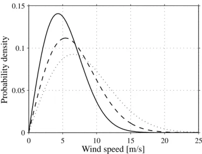
The most commonly used probability density function to describe the wind speed is the Weibull functions [53]. The Weibull distribution is described by the following probability density function f(w) = k c w c k−1 e−(w/c)k (2.1) where k is a shape parameter, cis a scale parameter and w is the wind speed. Thus, the average wind speed (or the expected wind speed),w, can be calculated from
w= ∞ 0 wf(w)dw= c kΓ 1 k (2.2) whereΓis Euler’s gamma function, i.e.,
Γ(z) =
∞
0
tz−1e−tdt. (2.3)
If the shape parameter equals 2, the Weibull distribution is known as the Rayleigh distribu-tion. For the Rayleigh distribution the scale factor, c, given the average wind speed can be found from (k=2, andΓ(12) = √π)
c= √2
πw. (2.4)
In Fig. 2.1, the wind speed probability density function of the Rayleigh distribution is plotted. The average wind speeds in the figure are 5.4 m/s, 6.8 m/s, and 8.2 m/s. A wind speed of 5.4 m/s correspond to a medium wind speed site in Sweden [100], while 8–9 m/s are wind speeds available at sites located outside the Danish west coast [24].
0 5 10 15 20 25 0 0.05 0.1 0.15 Wind speed [m/s] Probability density
Fig. 2.1. Probability density of the Rayleigh distribution. The average wind speeds are 5.4 m/s (solid), 6.8 m/s (dashed) and 8.2 m/s (dotted).
2.1.2
Aerodynamic Power Control
At high wind speeds it is necessary to limit the input power to the wind turbine, i.e., aero-dynamic power control. There are three major ways of performing the aeroaero-dynamic power control, i.e., by stall, pitch, or active stall control. Stall control implies that the blades are designed to stall in high wind speeds and no pitch mechanism is thus required [11].
Pitch control is the most common method of controlling the aerodynamic power gen-erated by a turbine rotor, for newer larger wind turbines. Almost all variable-speed wind turbines use pitch control. Below rated wind speed the turbine should produce as much power as possible, i.e., using a pitch angle that maximizes the energy capture. Above rated wind speed the pitch angle is controlled in such a way that the aerodynamic power is at its rated [11]. In order to limit the aerodynamic power, at high wind speeds, the pitch angle is controlled to decrease the angle of attack, i.e., the angle between the chord line of the blade and the relative wind direction [53]. It is also possible to increase the angle of attack towards stall in order to limit the aerodynamic power. This method can be used to fine-tune the power level at high wind speeds for fixed-speed wind turbines. This control method is known as
active stallorcombi stall[11].
2.1.3
Aerodynamic Conversion
Some of the available power in the wind is converted by the rotor blades to mechanical power acting on the rotor shaft of the WT. For steady-state calculations of the mechanical power from a wind turbine, the so calledCp(λ, β)-curve can be used. The mechanical power,Pmech, can be determined by [53] Pmech= 1 2ρArCp(λ, β)w3 (2.5) λ= Ωrrr w (2.6)
whereCpis the power coefficient,β is the pitch angle,λis the tip speed ratio,wis the wind speed, Ωr is the rotor speed (on the low-speed side of the gearbox), rr is the rotor-plane radius,ρis the air density andAris the area swept by the rotor. In Fig. 2.2, an example of a
Cp(λ, β)curve and the shaft power as a function of the wind speed for rated rotor speed, i.e., a fixed-speed wind turbine, can be seen. In Fig. 2.2b) the solid line corresponds to a fixed
0 5 10 15 20 0 0.1 0.2 0.3 0.4 0.5 5 10 15 20 25 0 20 40 60 80 100 120
Tip speed ratio
Cp ( λ ) a) Wind speed [m/s] Po wer [%] b)
Fig. 2.2. a) The power coefficient,Cp, as a function of the tip speed ratio,λ. b) Mechanical power as
a function of wind speed at rated rotor speed (solid line is fixed pitch angle, i.e., stall control and dashed line is active stall).
pitch angle,β, while dashed line corresponds to a varyingβ(active stall).
Fig. 2.3 shows an example of how the mechanical power, derived from the Cp(λ, β) curve, and the rotor speed vary with the wind speed for a variable-speed wind turbine. The rotor speed in the variable-speed area is controlled in order to keep the optimal tip speed ratio, λ, i.e., Cp is kept at maximum as long as the power or rotor speed is below its rated values. As mentioned before, the pitch angle is at higher wind speeds controlled in order to limit the input power to the wind turbine, when the turbine has reached the rated power. As seen in Fig. 2.3b) the turbine in this example reaches the rated power, 1 p.u., at a wind speed of approximately 13 m/s. Note that there is a possibility to optimize the radius of the wind turbines rotor to suit sites with different average wind speeds. For example, if the rotor radius,rr, is increased, the output power of the turbine is also increased, according to (2.5). This implies that the nominal power will be reached for a lower wind speed, referred to Fig. 2.3b). However, increasing the rotor radius implies that for higher wind speed the output power must be even more limited, e.g., by pitch control, so that the nominal power of the generator is not exceeded. Therefore, there is a trade-off between the rotor radius and the nominal power of the generator. This choice is to a high extent dependent on the average wind speed of the site.
2.2
Wind Turbine Systems
Wind turbines can operate with either fixed speed (actually within a speed range about 1 %) or variable speed. For fixed-speed wind turbines, the generator (induction generator) is
di-5 10 15 20 25 10 15 20 25 5 10 15 20 25 0 20 40 60 80 100 Rotor speed [rpm] a) Wind speed [m/s] Wind speed [m/s] Po wer [%] b)
Fig. 2.3. Typical characteristic for a variable-speed wind turbine. a) Rotor speed as a function of wind speed. b) Mechanical power as a function of wind speed.
rectly connected to the grid. Since the speed is almost fixed to the grid frequency, and most certainly not controllable, it is not possible to store the turbulence of the wind in form of rotational energy. Therefore, for a fixed-speed system the turbulence of the wind will result in power variations, and thus affect the power quality of the grid [77]. For a variable-speed wind turbine the generator is controlled by power electronic equipment, which makes it pos-sible to control the rotor speed. In this way the power fluctuations caused by wind variations can be more or less absorbed by changing the rotor speed [82] and thus power variations originating from the wind conversion and the drive train can be reduced. Hence, the power quality impact caused by the wind turbine can be improved compared to a fixed-speed tur-bine [58].
The rotational speed of a wind turbine is fairly low and must therefore be adjusted to the electrical frequency. This can be done in two ways: with a gearbox or with the number of pole pairs of the generator. The number of pole pairs sets the mechanical speed of the generator with respect to the electrical frequency and the gearbox adjusts the rotor speed of the turbine to the mechanical speed of the generator.
In this section the following wind turbine systems will be presented: 1. Fixed-speed wind turbine with an induction generator.
2. Variable-speed wind turbine equipped with a cage-bar induction generator or synchro-nous generator.
3. Variable-speed wind turbine equipped with multiple-pole synchronous generator or multiple-pole permanent-magnet synchronous generator.
4. Variable-speed wind turbine equipped with a doubly-fed induction generator.
There are also other existing wind turbine concepts; a description of some of these systems can be found in [36].
2.2.1
Fixed-Speed Wind Turbine
For the fixed-speed wind turbine the induction generator is directly connected to the electrical grid according to Fig. 2.4. The rotor speed of the fixed-speed wind turbine is in principle
IG Soft starter Gear-box Transformer Capacitor bank
Fig. 2.4. Fixed-speed wind turbine with an induction generator.
determined by a gearbox and the pole-pair number of the generator. The fixed-speed wind turbine system has often two fixed speeds. This is accomplished by using two generators with different ratings and pole pairs, or it can be a generator with two windings having different ratings and pole pairs. This leads to increased aerodynamic capture as well as reduced magnetizing losses at low wind speeds. This system (one or two-speed) was the “conventional” concept used by many Danish manufacturers in the 1980s and 1990s [36].
2.2.2
Variable-Speed Wind Turbine
The system presented in Fig. 2.5 consists of a wind turbine equipped with a converter con-nected to the stator of the generator. The generator could either be a cage-bar induction
Power electronic converter G Transformer Gear-box = = ≈ ≈
Fig. 2.5. Variable-speed wind turbine with a synchronous/induction generator.
generator or a synchronous generator. The gearbox is designed so that maximum rotor speed corresponds to rated speed of the generator. Synchronous generators or permanent-magnet synchronous generators can be designed with multiple poles which implies that there is no need for a gearbox, see Fig. 2.6. Since this “full-power” converter/generator system is com-monly used for other applications, one advantage with this system is its well-developed and robust control [7, 39, 61]. A synchronous generator with multiple poles as a wind turbine generator is successfully manufactured by Enercon [25].
Power electronic converter SG Transformer = = ≈ ≈
Fig. 2.6. Variable-speed direct-driven (gear-less) wind turbine with a synchronous generator (SG).
2.2.3
Variable-Speed Wind Turbine with Doubly-Fed Induction
Gener-ator
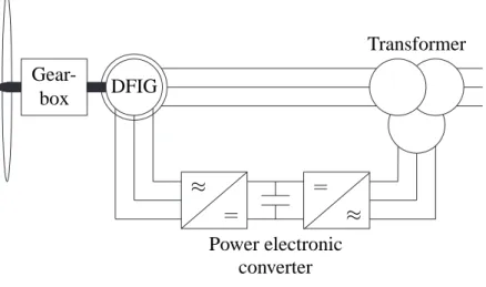
This system, see Fig. 2.7, consists of a wind turbine with doubly-fed induction generator. This means that the stator is directly connected to the grid while the rotor winding is con-nected via slip rings to a converter. This system have recently become very popular as
gen-Power electronic converter DFIG Transformer Gear-box = = ≈ ≈
Fig. 2.7. Variable-speed wind turbine with a doubly-fed induction generator (DFIG).
erators for variable-speed wind turbines [36]. This is mainly due to the fact that the power electronic converter only has to handle a fraction (20–30%) of the total power [36, 110]. Therefore, the losses in the power electronic converter can be reduced, compared to a system where the converter has to handle the total power, see Chapter 3. In addition, the cost of the converter becomes lower.
There exists a variant of the DFIG method that uses controllable external rotor resistances (compare to slip power recovery). Some of the drawbacks of this method are that energy is unnecessary dissipated in the external rotor resistances and that it is not possible to control the reactive power.
Manufacturers, that produce wind turbines with the doubly-fed induction machine as generator are, for example, DeWind, GE Wind Energy, Nordex, and Vestas [19, 29, 73, 105].
2.3
Doubly-Fed Induction Generator Systems for Wind
Tur-bines
For variable-speed systems with limited variable-speed range, e.g. ±30% of synchronous speed, the DFIG can be an interesting solution [61]. As mentioned earlier the reason for this is that power electronic converter only has to handle a fraction (20–30%) of the total power [36, 110]. This means that the losses in the power electronic converter can be reduced compared to a system where the converter has to handle the total power. In addition, the cost of the converter becomes lower. The stator circuit of the DFIG is connected to the grid while the rotor circuit is connected to a converter via slip rings, see Fig. 2.8. A more detailed picture
Converter
Fig. 2.8. Principle of the doubly-fed induction generator.
of the DFIG system with a back-to-back converter can be seen in Fig. 2.9. The back-to-back converter consists of two converters, i.e., machine-side converter and grid-side converter, that are connected “back-to-back.” Between the two converters a dc-link capacitor is placed, as energy storage, in order to keep the voltage variations (or ripple) in the dc-link voltage small. With the machine-side converter it is possible to control the torque or the speed of
DFIG Grid converter converter Grid-side Machine-side dc link ≈ ≈ = =
Fig. 2.9. DFIG system with a back-to-back converter.
the DFIG and also the power factor at the stator terminals, while the main objective for the grid-side converter is to keep the dc-link voltage constant. The speed–torque characteristics of the DFIG system can be seen in Fig. 2.10 [61]. As also seen in the figure, the DFIG can operate both in motor and generator operation with a rotor-speed range of±Δωmax
r around the synchronous speed,ω1.
Motor Generator T ωr ω1 2Δωrmax
Fig. 2.10. Speed–torque characteristics of a DFIG.
A typical application, as mentioned earlier, for DFIG is wind turbines, since they operate in a limited speed range of approximately±30%. Other applications, besides wind turbines, for the DFIG systems are, for example, flywheel energy storage system [4], stand-alone diesel systems [78], pumped storage power plants [6, 43], or rotating converters feeding a railway grid from a constant frequency public grid [61].
2.3.1
Equivalent Circuit of the Doubly-Fed Induction Generator
The equivalent circuit of the doubly-fed induction generator, with inclusion of the magnetiz-ing losses, can be seen in Fig. 2.11. This equivalent circuit is valid for one equivalent Y phase and for steady-state calculations. In the case that the DFIG isΔ-connected the machine can still be represented by this equivalent Y representation. In this section the jω-method is adopted for calculations. Note, that if the rotor voltage, Vr, in Fig. 2.11, is short circuited
+ + − − Rs jω1Lsλ jω1Lm Rm Rr/s jω1Lrλ Is Ir Vs IRm Vr s
Fig. 2.11. Equivalent circuit of the DFIG.
the equivalent circuit for the DFIG becomes the ordinary equivalent circuit for a cage-bar induction machine. Applying Kirchhoff’s voltage law to the circuit in Fig. 2.11 yields [87]
Vs=RsIs+jω1LsλIs+jω1Lm(Is+Ir+IRm) (2.7) Vr s = Rr s Ir+jω1LrλIr+jω1Lm(Is+Ir+IRm) (2.8) 0 =RmIRm+jω1Lm(Is+Ir+IRm) (2.9)
where the following notation is used.
Vs stator voltage; Rs stator resistance; Vr rotor voltage; Rr rotor resistance;
Is stator current; Rm magnetizing resistance; Ir rotor current; Lsλ stator leakage inductance; IRm magnetizing resistance current; Lrλ rotor leakage inductance;
ω1 stator frequency; Lm magnetizing inductance;
s slip. The slip,s, equals
s= ω1−ωr ω1
= ω2
ω1
(2.10) whereωr is the rotor speed andω2 is the slip frequency. Moreover, if the air-gap flux, stator flux and rotor flux are defined as
Ψm =Lm(Is+Ir+IRm) (2.11)
Ψs =LsλIs+Lm(Is+Ir+IRm) =LsλIs+ Ψm (2.12)
Ψr =LrλIr+Lm(Is+Ir+IRm) = LrλIr+ Ψm (2.13)
the equations describing the equivalent circuit, i.e., (2.7)–(2.9), can be rewritten as
Vs=RsIs+jω1Ψs (2.14) Vr s = Rr s Ir+jω1Ψr (2.15) 0 =RmIRm +jω1Ψm. (2.16)
The resistive losses of the induction generator are
Ploss = 3
Rs|Is|2+Rr|Ir|2+Rm|IRm|
2 (2.17)
and it is possible to express the electro-mechanical torque,Te, as
Te= 3npIm ΨmI∗r = 3npIm ΨrI∗r (2.18) wherenp is the number of pole pairs. Table 2.1 shows some typical parameters of the induc-tion machine in per unit (p.u.).
TABLE2.1. TYPICALPARAMETERS OF THEINDUCTIONMACHINE IN P.U., [101].
Small Medium Large
Machine Machine Machine
4 kW 100 kW 800 kW
Stator and rotor resistance RsandRr 0.04 0.01 0.01 Leakage inductance Lsλ+Lrλ ≈Lσ 0.2 0.3 0.3
2.3.2
Power Flow
In order to investigate the power flow of the DFIG system the apparent power that is fed to the DFIG via the stator and rotor circuit has to be determined. The stator apparent powerSs and rotor apparent powerSrcan be found as
Ss= 3VsI∗s = 3Rs|Is|2+j3ω1Lsλ|Is|2+j3ω1ΨmI∗s (2.19) Sr = 3VrI∗r = 3Rr|Ir|2+j3ω1sLrλ|Ir|2+j3ω1sΨmI∗r (2.20) which can be rewritten, using the expressions in the previous section, as
Ss = 3Rs|Is|2 +j3ω1Lsλ|Is|2+j3ω1| Ψm|2 Lm + 3Rm|IRm| 2− j3ω1ΨmI∗r (2.21) Sr = 3Rr|Ir| 2+ j3ω1sLrλ|Ir| 2 + j3ω1sΨmI∗r. (2.22)
Now the stator and rotor power can be determined as
Ps = Re [Ss] = 3Rs|Is| 2+ 3 Rm|IRm| 2+ 3 ω1Im [ΨmI∗r]≈3ω1Im [ΨmI∗r] (2.23) Pr = Re [Sr] = 3Rr|Ir|2−3ω1sIm [ΨmI∗r]≈ −3ω1sIm [ΨmI∗r] (2.24) where the approximations are because the resistive losses and the magnetizing losses have been neglected. From the above equations the mechanical power produced by the DFIG can be determined as the sum of the stator and rotor power as
Pmech= 3ω1Im [ΨmI∗r]−3ω1sIm [ΨmI∗r] = 3ωrIm [ΨmI∗r]. (2.25) Then, by dividing Pmech with mechanical rotor speed, ωm = ωr/np, the produced electro-mechanical torque, as given in (2.18), can be found. Moreover, this means that Ps ≈
Pmech/(1 −s) and Pr ≈ −sPmech/(1− s). In Fig. 2.12 the power flow of a “lossless” DFIG system can be seen. In the figure it can be seen how the mechanical power divides
Pmech Pmech Pmech/(1−s) sPmech/(1−s) DFIG Converter Grid
Fig. 2.12. Power flow of a “lossless” DFIG system.
between the stator and rotor circuits and that it is dependent on the slip. Moreover, the rotor power is approximately minus the stator power times the slip: Pr ≈ −sPs. Therefore, as mentioned earlier, the rotor converter can be rated as a fraction of the rated power of the DFIG if the maximum slip is low.
An example of how the stator and rotor powers depend on the slip is shown in Table 2.2. It can be seen in the table that the power through the converter, given the mechanical power,
TABLE2.2. EXAMPLE OF THEPOWERFLOW FORDIFFERENTSLIPS OF THEDFIGSYSTEM.
slip,s, [%] rotor speed,ωr, [p.u.] rotor power,Pr stator power,Ps
0.3 0.7 −0.43·Pmech. 1.43·Pmech.
0 1.0 0 Pmech.
−0.3 1.3 0.23·Pmech. 0.77·Pmech.
is higher for positive slips (ωr < ω1). This is due to the factor 1/(1−s)in the expressions for the rotor power. However, for a wind turbine, the case is not as shown in Table 2.2. For a wind turbine, in general, at low mechanical power the slip is positive and for high mechanical power the slip is negative, as seen in Fig. 2.13. The figure is actually the same as Fig. 2.3, but the stator and rotor power of the DFIG system is also shown and instead of the rotor speed the slip is shown. In the figure it is assumed that the gearbox ratio is set in such a way that
5 10 15 20 25 −50 −25 0 25 50 5 10 15 20 25 0 20 40 60 80 100 Slip [%] a) Wind speed [m/s] Wind speed [m/s] Po wer [%] b)
Fig. 2.13. Typical characteristic for a variable speed DFIG wind turbine. a) Slip as a function of wind speed. b) Mechanical power (dotted), rotor power (solid) and stator power (dashed) as a function of wind speed.
the average value of the rotor-speed range corresponds to synchronous speed of the DFIG. Moreover, for the wind turbine in Fig. 2.13 the stator power is at maximum only 0.7 times the rated power.
2.3.3
Stator-to-Rotor Turns Ratio
Since the losses in the power electronic converter depend on the current through the valves, it is important to have a stator-to-rotor turns ratio of the DFIG that minimizes the rotor current without exceeding the maximum available rotor voltage. In Fig. 2.14 a transformer is placed between the rotor circuit and the converter. The transformer is to highlight and indicate the stator-to-rotor turns ratio, but it does not exist in reality.
For example, if the stator-to-rotor turns ratio, ns/nr, is 0.4, the rotor current is ap-proximately 0.4 times smaller than the stator current, if the magnetizing current is ne-glected. Moreover, if the slipsof the DFIG is 30%, the rotor voltage will approximately be
Vrotor
R = s/(ns/nr)Vs = 0.3/0.4Vs = 0.75Vs, i.e., 75% of the stator voltage, which leaves room for a dynamic control reserve. Note thatVRrotor = (nr/ns)VR is the actual (physical)
Converter DFIG
ns/nr
Fig. 2.14. Stator-to-rotor turns ratio indicated with a “virtual” transformer.
rotor voltage, whileVRis rotor voltage referred to the stator circuit. In this thesis, all rotor variables and parameters are referred to the stator circuit if not otherwise stated.
2.3.4
Lowering Magnetizing Losses
In an ordinary induction machine drive the stator is fed by a converter, which means that it is possible to reduce the losses in the machine by using an appropriate flux level. At low loads it is possible to reduce the flux level, which means that the magnetizing losses are lowered, leading to a better efficiency. However, in the DFIG system the stator is connected to the grid, and accordingly the flux level is closely linked to the stator voltage. Still, for the DFIG system there are, at least, two methods to lower the magnetizing losses of the DFIG. This can be done by:
1. short-circuiting the stator of the induction generator at low wind speeds, and trans-mitting all the turbine power through the converter. This set-up is referred to as the
short-circuited DFIG.
2. having the stator Δ-connected at high wind speeds and Y-connected at low wind speeds; referred to as theY-Δ-connected DFIG.
The influence that these two methods have on the overall efficiency of a DFIG system will be further analyzed in Chapter 3. A brief description of these two systems follows:
“Short-Circuited DFIG”
Fig. 2.15 shows a diagram of the “short-circuited DFIG.” In the figure two switches can be seen. Switch S2 is used to disconnect the turbine from the grid and switch S1 is then used to short-circuit the stator of the DFIG. Now the turbine is operated as a cage-bar induction machine, except that the converter is connected to the rotor circuit instead of the stator circuit. This means, that in this operating condition, the DFIG can be controlled in a similar way as an ordinary cage-bar induction generator. For instance, at low wind speeds the flux level in the generator can be lowered.
Y-Δ-connected DFIG
Fig. 2.16 presents a set-up of the Y-Δ-connected DFIG. As shown in the figure, a device for changing between Y andΔconnection has been inserted in the stator circuit. Before a
Power electronic converter DFIG Transformer S1 S2 = = ≈ ≈
Fig. 2.15. Principle of the “short-circuited DFIG.”
Power electronic converter DFIG Transformer Y/Δ S1 = = ≈ ≈
Fig. 2.16. Principle of the Y-Δ-connected DFIG.
change from Y toΔconnection (or vice versa) the power of the turbine is reduced to zero and the switch S1 disconnects the stator circuit from the grid. Then the stator circuit is connected inΔ(or vice versa) and the turbine is synchronized to the grid.
2.3.5
Other Types of Doubly-Fed Machines
In this section a short presentation of other kinds of doubly-fed machines is made: a cascaded doubly-fed induction machine, a single-frame cascaded doubly-fed induction machine, a brushless doubly-fed induction machine, and a doubly-fed reluctance machine.
Cascaded Doubly-Fed Induction Machine
The cascaded doubly-fed induction machine consists of two doubly-fed induction machines with wound rotors that are connected mechanically through the rotor and electrically through the rotor circuits. See Fig. 2.17 for a principle diagram. The stator circuit of one of the ma-chines is directly connected to the grid while the other machine’s stator is connected via a
Converter
Fig. 2.17. Principle of cascaded doubly-fed induction machine.
converter to the grid. Since the rotor voltages of both machines are equal, it is possible to control the induction machine that is directly connected to the grid with the other induction machine.
It is possible to achieve decoupled control of active and reactive power of the cascaded doubly-fed induction machine in a manner similar to the doubly-fed induction machine [47]. It is doubtful whether it is practical to combine two individual machines to form a cas-caded doubly-fed induction machine, even though it is the basic configuration of doubly-fed induction machine arrangement. Due to a large amount of windings, the losses are expected to be higher than for a standard doubly-fed induction machine of a comparable rating [48]. Single-Frame Cascaded Doubly-Fed Induction Machine
The single-frame cascaded doubly-fed induction machine is a cascaded doubly-fed induction machine, but with the two induction machines in one common frame. Although this machine is mechanically more robust than the cascaded doubly-fed induction machine, it suffers from comparatively low efficiency [48].
Brushless Doubly-Fed Induction Machine
This is an induction machine with two stator windings in the same slot. That is, one winding for the power and one winding for the control. See Fig. 2.18 for a principle sketch. To avoid a direct transformer coupling between the two-stator windings, they can not have the same number of pole pairs. Furthermore, to avoid unbalanced magnetic pull on the rotor the difference between the pole pairs must be greater than one [106]. The number of poles in the rotor must equal the sum of the number of poles in the two stator windings [106]. For further information and more details, see [106, 108, 111].
Doubly-Fed Reluctance Machine
The stator of the doubly-fed reluctance machine is identical to the brushless doubly-fed in-duction machine, while the rotor is based on the principle of reluctance. An equivalent circuit with constant parameters can be obtained for the doubly-fed reluctance machine, in spite the
Converter
Fig. 2.18. Principle of the brushless doubly-fed induction machine.
fact that the machine is characterized by a pulsating air-gap flux. It has almost the same equivalent circuit as the standard doubly-fed induction generator [109].
Chapter 3
Energy Efficiency of Wind Turbines
The purpose of this chapter is to investigate the energy efficiency of the DFIG system and to relate this study to other types of WTs with various electrical systems. This study focuses on 1) reducing the magnetizing losses of the DFIG system, 2) influence of the converter’s size on the energy production (i.e., smaller converter implies a smaller variable-speed range for the DFIG system) and finally 3) comparison of the DFIG system to other electrical systems. In order to make the comparison as fair as possible the base assumption used in this work is that the maximum (average) shaft torque of the wind turbine systems used should be the same. Moreover, the rated WT power used in this chapter is 2 MW.
3.1
Determination of Power Losses
Steady-state calculations are carried out in this section in order to determine the power losses of the DFIG system. Moreover, in order to compare the performance of the DFIG system, the power losses of other systems with induction generators will also be presented. The following systems are included in this study:
• FSIG 1 system— Fixed-speed system, as described in Section 2.2.1, with one genera-tor.
• FSIG 2 system— Fixed-speed system, as described in Section 2.2.1, with two gener-ators or a pole-pair changing mechanism.
• VSIG system— Variable-speed system with an induction generator and a full-power converter, as described in Section 2.2.2.
• DFIG system— Variable-speed system with a DFIG, as described in Section 2.2.3. The following losses are taken into account: aerodynamic losses, gearbox losses, gener-ator losses and converter losses.
3.1.1
Aerodynamic Losses
Fig. 3.1 shows the turbine power as a function of wind speed both for the fixed-speed and variable-speed systems. In the figure it is seen that the fixed-speed system with only one generator has a lower input power at low wind speeds. The other systems produce almost
5 10 15 20 25 0 20 40 60 80 100 T u rbine p o w er [%] Wind speed [m/s]
Fig. 3.1. Turbine power. The power is given in percent of maximum shaft power. The solid line corresponds to the variable-speed systems (VSIG and DFIG) and the two-speed system (FSIG 2). The dotted line corresponds to a fixed-speed system (FSIG 1).
identical results. In order to calculate the power in Fig. 3.1, a so-calledCp(λ, β)-curve, as described in Section 2.1.3, derived using blade-element theory has been used used.
In order to avoid making the results dependent on the torque, speed and pitch control strategy, that vary from turbine to turbine, and anyway the settings used by the manufacturers are not in detail known by the authors, only the average wind speed is used in the calculations, i.e., the influence of the turbulence is ignored. The interested reader can find information of the influence of the turbulence on the energy production in [69].
3.1.2
Gearbox Losses
One way to estimate the gearbox losses,Ploss,GB, is, [33],
Ploss,GB=ηPlowspeed+ξPnom
Ωr
Ωr,nom
(3.1) whereηis the gear-mesh losses constant andξ is a friction constant. According to [34], for a 2-MW gearbox, the constants η = 0.02and ξ = 0.005 are reasonable. In Fig. 3.2 the gearbox losses are shown for the investigated systems.
3.1.3
Induction Generator Losses
In order to calculate the losses of the generator, the equivalent circuit of the induction gener-ator, with inclusion of magnetizing losses, has been used, see Section 2.3.1.
For the DFIG system, the voltage drop across the slip rings has been neglected. More-over, the stator-to-rotor turns ratio for the DFIG is adjusted so that maximum rotor voltage is 75% of the rated grid voltage. This is done in order to have safety margin, i.e., a dynamic reserve to handle, for instance, a wind gust. Observe that instead of using a varying turns ratio, the same effect can also be obtained by using different rated voltages on the rotor and stator [81].
4 6 8 10 12 14 16 0 0.5 1 1.5 2 2.5 3 Gearbox losses [%] Wind speed [m/s] FSIG 2 FSIG 1 VSIG
Fig. 3.2. Gearbox losses. The losses are given in percent of maximum shaft power. The solid line corresponds to the variable-speed systems (VSIG and DFIG). The dotted lines correspond to fixed-speed systems, i.e., FSIG 1 and 2 (both one-speed and two-speed generators).
In Fig. 3.3 the induction generator losses of the DFIG system are shown. The reason that the generator losses are larger for high wind speeds for the VSIG system compared to the DFIG system is that the gearbox ratio is different between the two systems. This implies that the shaft torque of the generators will be different for the two systems, given the same input power. It can also be noted that the losses of the DFIG are higher than those of the
5 10 15 20 25 0 0.5 1 1.5 2 2.5 3 Generator losses [%] Wind speed [m/s] DFIG VSIG FSIG 1 & 2
Fig. 3.3. Induction generator losses. The losses are given in percent of maximum shaft power. DFIG is solid, dashed is the variable-speed system (VSIG) and dotted are the fixed-speed systems (FSIG 1 and 2).
VSIG for low wind speeds. The reason for this is that the flux level of the VSIG system has been optimized from an efficiency point of view while for the DFIG system the flux level is almost fixed to the stator voltage. This means that for the VSIG system a lower flux level is
used for low wind speeds, i.e., the magnetizing losses are reduced.
For the IGs used in this chapter operated at 690 V 50 Hz and with a rated current of 1900 A and 390 A, respectively, the following parameters are used:
2-MW power: See Appendix B.1.
0.4-MW power: Rs = 0.04 p.u., Rr = 0.01 p.u., Rm = 192 p.u., Lsλ = 0.12 p.u.,
Lrλ = 0.04p.u.,Lm = 3.7p.u. andnp = 3.
3.1.4
Converter Losses
In order to be able to feed the IG with a variable voltage and frequency source, the IG can be connected to a pulse-width modulated (PWM) converter. In Fig. 3.4, an equivalent circuit of the converter is drawn, where each transistor, T1 to T6, is equipped with a reverse diode. A PWM circuit switches the transistors to on and off states. The duty cycle of the transistor and the diode determines whether the transistor or a diode is conducting in a transistor leg (e.g., T1 and T4). T1 T2 T3 T4 T5 T6 VCE0 rCE VT0 rT ⇔ ⇔
Fig. 3.4. Converter scheme.
The losses of the converter can be divided into switching losses and conducting losses. The switching losses of the transistors are the turn-on and turn-off losses. For the diode the switching losses mainly consist of turn-off losses [103], i.e., reverse-recovery energy. The turn-on and turn-off losses for the transistor and the reverse-recovery energy loss for a diode can be found from data sheets. The conducting losses arise from the current through the transistors and diodes. The transistor and the diode can be modeled as constant voltage drops,
VCE0 andVT0, and a resistance in series,rCE andrT, see Fig. 3.4. Simplified expressions of the transistor’s and diode’s conducting losses, for a transistor leg, are (with a third harmonic voltage injection) [2] Pc,T = VCE0Irms √ 2 π + IrmsVCE0micos(φ) √ 6 + rCEIrms2 2 + rCEIrms2 mi √ 3 cos(φ)6π − 4rCEIrms2 micos(φ) 45π√3 (3.2) Pc,D= VT0Irms √ 2 π − IrmsVT0√micos(φ) 6 + rTIrms2 2 − √rTIrms2 mi 3 cos(φ)6π + 4rTIrms2 micos(φ) 45π√3 (3.3)
whereIrmsis the root mean square (RMS) value of the (sinusoidal) current to the grid or the generator, mi is the modulation index, and φis the phase shift between the voltage and the current.
Since, for the values in this chapter, which are based on [89, 90, 91, 92] (see Table 3.1 for actual values), rIGBT = rCE ≈ rT and VIGBT = VCEO ≈ VT O. Hence, it is possible to reduce the loss model of the transistor and the diode to the same model. The conduction
TABLE3.1. CONVERTERCHARACTERISTICDATA(IGBTANDINVERSEDIODE).
Nominal current IC,nom 500 A 1200 A 1800 A 2400 A
Operating dc-link voltage VCC 1200 V 1200 V 1200 V 1200 V
VCEO 1.0 V 1.0 V 1.0 V 1.0 V
Lead resistance (IGBT) rCE 3 mΩ 1.5 mΩ 1 mΩ 0.8 mΩ Turn-on and turn-off
Eon+Eoff 288 mJ 575 mJ 863 mJ 1150 mJ energy (IGBT)
VT O 1.1 V 1.1 V 1.1 V 1.1 V
Lead resistance (diode) rT 2.6 mΩ 1.5 mΩ 1.0 mΩ 0.8 mΩ Reverse recovery
Err 43 mJ 86 mJ 128 mJ 171 mJ
energy (diode)
losses can, with the above-mentioned approximation, be written as
Pc=Pc,T+Pc,D =VIGBT
2√2
π Irms+rIGBTI
2
rms. (3.4)
The switching losses of the transistor can be considered to be proportional to the current, for a given dc-link voltage, as is assumed here [2]. This implies that the switching losses from the transistor and the inverse diode can be expressed as
Ps,T = (Eon+Eoff) 2√2 π Irms IC,nom fsw ≈Vsw,T 2√2 π Irms (3.5) Ps,D =Err 2√2 π Irms IC,nom fsw ≈Vsw,D 2√2 π Irms (3.6)
whereEonandEoff are the turn-on and turn-off energy losses, respectively, for the transistor,
Erris the reverse recovery energy for the diode andIC,nomis the nominal current through the transistor. In the equations above, two voltage drops,Vsw,T andVsw,D, have been introduced. This is possible since the ratios(Eon+Eoff)/IC,nomandErr/IC,nomare practically constant for all the valves in Table 3.1. This means that for a given dc-link voltage and switching frequency (which both are assumed in this thesis), the switching losses of the IGBT and diode can be modeled as a constant voltage drop that is independent of the current rating of the valves. The switching frequency used in this thesis is 5 kHz. Moreover, since the products
rCEIC,nom andrTIC,nom also are practically constant and equal to each other, it is possible to determine a resistance,rIGBT,1A, that is valid for a nominal currentIC,nom = 1A. Then, the resistance of a specific valve can be determined fromrIGBT =rIGBT,1A/IC,nom, where
IC,nom is the nominal current of the valve. In this thesis,IC,nom is chosen asIC,nom = 2Irmsmax whereImax
rms is the maximum RMS value of the current in the valve. By performing the above simplification the model of the IGBT and valve can be scaled to an arbitrary rating. Using
the values given in Table 3.1 it is possible to determine the voltage dropsVsw,T = 2.5V and
Vsw,D = 0.38V, assuming a switching frequency of 5 kHz and the resistancerIGBT,1A =
1.76 Ω. When determiningVsw,T,Vsw,D, andrIGBT,1Athe average values of all of the valves
in Table 3.1 has been used. Now, the total losses from the three transistor legs of the converter become Ploss = 3(Pc+Ps,T+Ps,D) = 3 (VIGBT +Vsw,T +Vsw,D) 2√2 π Irms+rIGBTI 2 rms . (3.7)
The back-to-back converter can be seen as two converters which are connected together: the machine-side converter (MSC) and the grid-side converter (GSC). For the MSC, the current through the valves,Irms, is the stator current for the VSIG system or the rotor current for the DFIG system. One way of calculatingIrmsfor the GSC is by using the active current that is produced by the machine, adjusted with the ratio between machine-side voltage and the grid voltage. The reactive current can be freely chosen. Thus it is now possible to calculate the losses of the back-to-back converter as
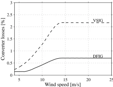
Ploss,converter =Ploss,GSC+Ploss,MSC. (3.8) The total converter losses are now presented as a function of wind speed in Fig. 3.5. From the figure it can, as expected, be noted that the converter losses in the DFIG system are
5 10 15 20 25 0 0.5 1 1.5 2 2.5 3 Con v erter losses [%] Wind speed [m/s] DFIG VSIG
Fig. 3.5. Converter losses. The losses are given in percent of maximum shaft power. DFIG is solid and VSIG is dashed.
much lower compared to the full-power converter system.
3.1.5
Total Losses
The total losses (aerodynamic, generator, converter, gearbox) are presented in Fig. 3.6. From the figure it can be noted that the DFIG system and the two-speed system (FSIG 2) has roughly the same total losses while the full-power converter system has higher total losses.