Research Institute of Industrial Economics P.O. Box 55665 SE-102 15 Stockholm, Sweden
[email protected] www.ifn.se
IFN Working Paper No. 799, 2009
Creative Destruction and Productive
Preemption
Pehr-Johan Norbäck, Lars Persson and
Creative Destruction and Productive Preemption
Pehr-Johan Norbäck
Research Institute of Industrial Economics (IFN) Lars Persson
Research Institute of Industrial Economics (IFN) and CEPR Roger Svensson
Research Institute of Industrial Economics (IFN) June 9, 2009
Abstract
We develop a theory of commercialization mode (entry or sale) of entrepreneurial inven-tions into oligopoly, and show that an invention of higher quality is more likely to be sold (or licensed) to an incumbent due to strategic product market e¤ects on the sales price. Moreover, preemptive acquisitions by incumbents are shown to stimulate the process of cre-ative destruction by increasing the entrepreneurial e¤ort allocated to high-quality invention projects. Using detailed data on patents granted to small …rms and individuals, we …nd evidence that high-quality inventions are often sold, and that they are sold under bidding competition.
Keywords: Acquisitions, Entrepreneurship, Innovation, Start-ups, Patent, Ownership, Quality
JEL classi…cation: G24, L1, L2, M13, O3
We have bene…tted from useful comments from Marcus Asplund, Magnus Henrekson, Jim Levinsohn, Ho-daka Morita, Sören-Bo Nielsen and Marie Thursby, and participants in seminars at IIOC Conference 2009, IFN Stockholm Conference 2007, Copenhagen Bussines School, Tilburg University and Royal Institute of Technology (Stockholm). Financial support from Jan Wallander’s and Tom Hedelius’Research Foundation is gratefully ac-knowledged. This paper was written within the Gustaf Douglas Research Program on Entrepreneurship. Email: [email protected], [email protected].
1. Introduction
Schumpeter (1942) argued that the ongoing process where new inventions create ”monopoly rents” for entrepreneurs while reducing rents for incumbentfirms is central for sustained growth in a market economy. This process of ”creative destruction” and its welfare implications has been studied in formal theory in the case where an entrepreneur commercializes the invention by entering the product market.1 However, if incumbent profits are hurt by entrepreneurial entry, incumbents should have an incentive to block entry by acquiring these entrepreneurial firms (or their inventions). Indeed, entrepreneurial inventions are often sold or licensed to incumbent firms.2 Figure 1.1 shows the importance of commercialization by sale in the last decade by depicting the exit value through M&As (proxying for commercialization by sale to incumbents) and IPOs (proxying for commercialization by entry), respectively, in the US venture capital market.
The purpose of this paper is to study how the innovation process is affected by the fact that entrepreneurial entry might be blocked by preemptive acquisitions by incumbents. To this end, we construct a theoretical model with the following ingredients: Initially, an entre-preneur decides how much to invest in research to discover an invention. Then, if successful, the entrepreneur could either enter the product market with the invention or sell it to one of many incumbentfirms competing to acquire the invention. Finally, firms compete in oligopoly fashion, thereby generating profits.
Wefirst show that the incentive for commercialization by sale relative to commercialization by entry increases with a higher quality of the invention. This occurs because higher invention quality increases entrants’ and acquirers’ profits in a similar fashion, but also reduces the profit when not acquiring the invention. This implies that the incumbent’s willingness to pay for the invention increases more than the entrant’s profit in quality and thereby the entrepreneur benefits from selling the invention instead of entering the market.
We then turn to how the quality of an invention affects the research incentives. When the entrepreneur commercializes by entry, she will set the effort level such that the marginal cost of research equals the marginal change in product market profit as an entrant. When commercializing by sale, the marginal cost will be the same but the marginal revenue will be higher at a high level of quality. Once again, increased quality of the invention does not only increase the profit of an acquirer of the invention but will also decrease the profit of a
1 In the endogenous growth literature see, for instance, Aghion and Howitt (1992), Grossman and Helpman (1991), Segerstrom, Anant, and Dinopoulos (1990), and Howitt (2008) for an overview, and in the Industrial Organization literature see, for instance, Arrow (1962), Gilbert and Newberry (1982) and Gilbert (2006) for an overview.
2
Granstrand and Sjölander (1990) present evidence from Sweden, and Hall (1990) presents evidence from the US that firms acquire innovative targets to gain access to their technologies. Bloningen and Taylor (2000)find evidence from US high-tech industries offirms making a strategic choice between the acquisition of outside innovators and in-house R&D. In the biotech industry, Lerner and Merges (1998) note that acquisitions are important for know-how transfers. Baumol (2004) stresses the importance of the different roles played by small entrepreneurial firms and large established firms in the innovation process in the USA, where small entrepreneurialfirms create a large share of breakthrough innovations and large establishedfirms provide more routinized R&D.
0 5000 10000 15000 20000 25000 30000 1999 2000 2001 2002 2003 2004 2005 year Million USD Value of exits through M&A Value of exits Through IPO
Figure 1.1: The value of exits through M&A and IPO in the US. Source: Thomson Venture Economics/National Venture Capital Association.
non-acquirer. Both these effects will increase incumbents’ willingness to pay, thus driving the sales price above the entrepreneur’s profit as an entrant. Entrepreneurs who commercialize by sale therefore have a stronger incentive to develop high-quality inventions than entrepreneurs who commercialize by entry. Since preemptive incumbent acquisitions give entrepreneurs the incentive to increase their efforts in high-quality research projects, expected consumer welfare can be higher under commercialization by sale despite the risk of increased market power.
Next, we derive an estimation equation from the entrepreneur’s decision of commercialization (sale or entry), and test it on a detailed dataset on patents granted to Swedish small firms and individual inventors. We use forward patent citations as a proxy for the quality of the invention. Consistent with theory, we find that higher patent quality is conducive to commercialization by sale. The estimates show that if a patent receives one more forward citation in a five-year period, the probability of sale increases by aboutfive percentage points. Additional predictions of the model such as higher entry costs being conducive to sale are also supported by data. Importantly, our estimates identify preemptive bidding competition between incumbentfirms.
We undertake a number of extensions of the empirical analyses. These include estimating a multinomial logit model, a probit model with selection and a duration model to control for the fact the data include patents that are not commercialized. These extensions yield no qualitative changes in results and, in particular, forward citations remain conducive to commercialization by sale.
This paper relates to the literature studying which type of products will be sold on the market. In his seminal paper, Akerlof (1970) showed that informational asymmetries can give rise to adverse selection on markets, resulting in that only low-quality products will be sold.3 In
3
The existing empirical literature on the ”lemons” effect gives mixed evidence. For instance, Bond (1982) found no evidence, Genesove (1993) weak evidence, and Gilligan (2004) strong evidence of adverse
contrast, we show theoretically that when inventions are sold into oligopolistic markets, absent the information problem, product market externalities imply that only high-quality products will be sold on the market. We alsofind empirical evidence that only high-quality inventions are sold on the market, using patent data. However, these data also show that commercialization by sale takes longer than commercialization by entry; thus, the asymmetric information problem could materialize in the cost of sale preparation.
This paper also contributes to the literature on commercialization mode, which has shown how different types of transaction costs and entry costs affect the commercialization mode (see, for instance, Anton and Yao (1994), Gans and Stern (2000) and Gans et al. (2002)). We add to this literature by theoretically and empirically showing that when the invention will be commercialized under bidding competition in an oligopolistic market, the invention is more likely to be commercialized through a sale to an incumbent, the higher is its quality.
This paper also relates to the literature on auctions with externalities (see, for instance, Jehiel, Moldovanu and Stacchetti (1996, 1999)). We add to this literature by endogenizing the choice of whether to sell the asset or use it to compete with the potential bidders. Moreover, to our knowledge, we are thefirst to provide evidence of preemptive bidding competition.
Finally, this paper contributes to the literature on entrepreneurship (for overviews, see Audreatch and Achs (2005) and Bianchi and Henrekson (2005)), by constructing an oligopoly model where the equilibrium commercialization mode pattern, the acquisition price and the entrepreneur’s investments are endogenously determined.4
2. The theoretical model.
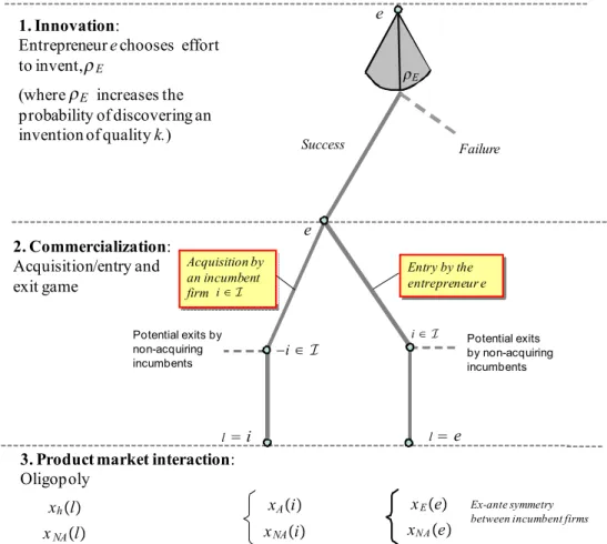
The interaction is illustrated in Figure 2.1. Consider a market served bynsymmetric incumbent firms. There is also an entrepreneur, denotede. In stage 1, the entrepreneur decides how much to invest in research, thereby affecting the probability of discovering an invention with a fixed quality k.5 In stage 2, if successful, the entrepreneur commercializes the invention into an innovation. She either sells the invention at afirst-price perfect information auction, where the
nincumbent firms are the potential buyers, or enters the product market. There may then be exits of incumbent firms. Finally, in stage 3, the active firms in the product market compete in oligopoly interaction, setting an actionxi. Following the literature, we will try use the term "invention" as long as k has not reached the market, while using the term "innovation" when
kis used in the product market.
selection.
4This paper is also related to the literature on patent licensing (for an overview, see Kamien (1992), and to the literature on the persistence of monopoly (see, for instance, Chen (2000) and Gilbert and Newbery (1982). However, to our knowledge, these literatures do not study how the trade-offbetween entry and sales (licence) for the potential entrant depends on the quality of the invention, which is the focus of our analysis.
5
The quality of an inventionkis for many types of inventionsfixed, such as for vaccines, or solutions to specific technical problems. However, for other inventions the quality of an invention can be affected, such as the capacity of a micro processor. We discuss the case where the entrepreneur chooses the quality in Section 5.1.
Success Failure
1. Innovation:
Entrepreneur echooses effort to invent,
(where increases the probability of discovering an invention of quality k.)
2. Commercialization:
Acquisition/entry and exit game
3. Product market interaction: Oligopoly e Acquisition by an incumbent firm Entry by the entrepreneur e l i l e Potential exits by non-acquiring incumbents Potential exits by non-acquiring incumbents −i∈ I i∈I i∈I E Ex-ante symmetry between incumbent firms
e xEe xNAe xAi xNAi xhl xNAl E E
2.1. Stage 3: Product-market equilibrium
Let the set of firms in the industry beJ =e∪I, whereI ={i1, i2...in}is the set of incumbent firms. Denote the owner of the entrepreneur’s invention,k, byl∈J. Using backward induction, we start with product market interaction wherefirm j chooses an actionxj ∈R+ to maximize its direct product market profit, πj(xj,x−j, l)−τ, which depends on its own and its rivals’ market actions, xj andx−j, the identity of the owner of the invention, l, and a fixed cost τ to serve the market. We may consider the action xj as setting a quantity or a price, as will be shown in later sections. We assume there to exist a unique Nash-Equilibrium,x∗(l), defined as:
πj(x∗j, x−∗j :l, k)≥πj(xj, x∗−j :l, k), ∀xj ∈R+, (2.1) where we assume the product market profits to be positive.
From (2.1), we can define a reduced-form product market profit for afirmj, taking as given ownership l:
πj(l)≡πj(x∗j(l), x∗−j(l), l). (2.2) The assumption that incumbents i1, i2, ..., in are symmetric before the acquisition takes place implies that we need only distinguish between two types of ownership; entrepreneurial ownership (l = e) and incumbent ownership (l = i). Note that there are then three types of firms of which to keep track, h = {e, A, N A}, i.e. the entrepreneurial firm (e), an acquiring incumbent (A) and the non-acquiring incumbents (N A).
We will now define the quality of an invention in this setting:
Definition 1. (i) dπA(i) dk >0, (ii) dπE(e) dk >0, and (iii) dπN A(l) dk <0, l=e, i.
Definitions 1 (i) and (ii) state that the reduced-form product market profit for the possessor is strictly increasing in the quality of the invention, whereas Definition 1 (iii) states that increased quality strictly decreases the rivals’ profits. This will, for instance, hold for a process innovation where a more drastic innovation leads to a larger reduction in the marginal cost of selling and producing for the product market.
Example 1 (The LC-model). As an example, we use a Linear-Cournot model (LC-model). This model is also used to derive more specific results. The oligopoly interaction in period 3 is Cournot competition in homogenous goods. The product market profit isπj = (P−cj)qj where firms face inverse demand P =a− 1sPNi=1qi, where a > 0 is a demand parameter, s may be interpreted as the size of the market, and N is the total number of firms in the market. In the LC-model, ownership of the invention reduces the marginal cost. Making a distinction between firm types, we have:
cN A=c, cA=c−k, cE =c−k. (2.3) In the LC model, (2.1) takes the form ∂πj
∂qj = P −cj −
qj
s = 0 ∀j, which can be solved for optimal quantities q∗(l). Noting that ∂πj
∂qj = 0 implies P −cj =−
qj
s, reduced-form profits are
πj(l) = 1s h
qj∗(l)
i2
, where q∗A(l) = sa−Nc+(iN)+1(i)k, qE∗(e) = sa−Nc+(eN)+1(e)k and qN A∗ (l) = sNa−(lc)+1−k for
of active incumbent firms. Holding the total number of firms N(l) fixed, it thus follows that reduced-form profits πj(l) fulfill Definition 1.
2.2. Stage 2: Commercialization
In stage 2, there isfirst an entry-acquisition game where the entrepreneur can decide whether to sell the invention to one of the incumbents or enter the market at afixed cost,G. Given the mode of commercialization of the invention, there may then be exits of non-acquiring incumbents.
The firm in possession of the invention is assumed to always make positive profits, i.e. we assume the quality of the inventionkto be sufficiently large so thatπA(l)> τ andπE(e)> τ+G holds. Non-acquiring incumbents will exit until the total number of firms on the market N(l)
fulfils theexit condition:
πN A(l:N(l))> τ , πN A(l:N(l) + 1)< τ , (2.4) wheremax:N(i) =n(i) and max:N(e) =n(e) + 1, where n(l)≤n.
The commercialization process is depicted as an auction wherenincumbents simultaneously post bids and the entrepreneur then either accepts or rejects these bids. If the entrepreneur rejects these bids, she will enter the market. Each incumbent announces a bid, bi, for the invention. b = (b1, ..bi.., bm) ∈ Rm is the vector of these bids. Following the announcement of b, the invention may be sold to one of the incumbents at the bid price, or remain in the ownership of entrepreneur e. If more than one bid is accepted, the bidder with the highest bid obtains the invention. If there is more than one incumbent with such a bid, each such incumbent obtains the invention with equal probability. The acquisition is solved for Nash equilibria in undominated pure strategies. There is a smallest amount, ε, chosen such that all inequalities are preserved ifεis added or subtracted.
There are three different valuations:
• vii in (2.5) is the value for an incumbent of obtaining k, when a rival incumbent would otherwise obtaink. Thefirst term shows the profit when possessing the inventionk. The second term shows the expected profit if a rival incumbent obtains k, where Γ is the transaction cost associated with acquiring the invention k, and λ(i) is the probability of staying in the market as a non-acquirer
vii=πA(i)−τ−Γ−λ(i) [πN A(i)−τ]. (2.5)
• vie in (2.6) is the value for an incumbent of obtaining k, when the entrepreneur would otherwise keep it. The profit for an incumbent of not obtaining inventionk is different in this case, due to the change of identity of thefirm that would otherwise possess the assets
vie=πA(i)−τ −Γ−λ(e) [πN A(e)−τ]. (2.6)
entering the market
ve=πE(e)−τ −G. (2.7)
Note that we assume that πE(i) = 0, so that the entrepreneur cannot enter the market without ownership of the invention. Note also that one possibility is that entry takes place through a sale to a largefirm outside this industry.
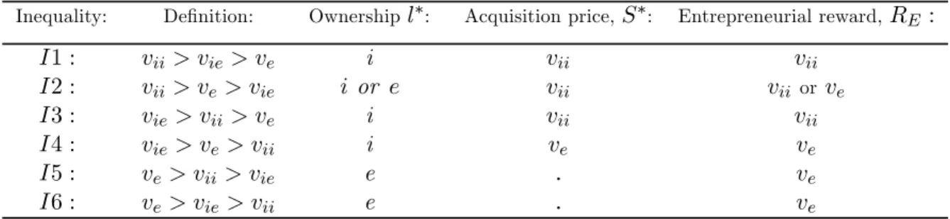
We can now proceed to solve for the Equilibrium Ownership Structure (EOS). Since incum-bents are symmetric, valuationsvii, vie and ve can be ordered in six different ways, as shown in table 2.1. These inequalities are useful for solving the model and illustrating the results. The following lemma can be stated:
Lemma 1. Equilibrium ownershipl∗, acquisition priceS∗ and entrepreneurial rewardRE are described in table 2.1:
Proof. See the Appendix.
Table 2.1: The equilibrium ownership structure and the acquisition price.
Inequality: Definition: Ownership l∗: Acquisition price,S∗: Entrepreneurial reward,RE :
I1 : vii> vie> ve i vii vii I2 : vii> ve> vie i or e vii vii or ve I3 : vie > vii> ve i vii vii I4 : vie > ve> vii i ve ve I5 : ve > vii> vie e
.
ve I6 : ve > vie> vii e.
veLemma 1 shows that when one of the inequalitiesI1, I3, orI4holds,kis obtained by one of the incumbents. Under I1 and I3, the acquiring incumbent pays the acquisition price S =vii, and S =ve under I4. WhenI5 or I6 holds, the entrepreneur keeps its assets. When I2 holds, there exist multiple equilibria. The last column summarizes the reward RE accruing to the entrepreneur.
2.3. Stage 1: Effort by the entrepreneur
In stage 1, entrepreneureinvests in researchρE to succeed with the inventionk. For simplicity, assume that the probability of succeeding with an invention is simply the effort, i.e. ρE ∈[0,1],
and that effort is associated with an increasing and convex cost y(ρ), i.e. y0(ρ) > 0, and
y00(ρ)>0. WithRE(l) given from Lemma 1,ΠE =ρERE(l)−y(ρE) is the expected net profit of undertaking a research effort for the entrepreneur. The optimal effort ρ∗E is given from:
dΠE
dρE =RE(l)−y
0(ρ∗
E(l)) = 0, (2.8)
with the associated second-order condition (omitting the ownership variablel), d2ΠE
dρ2
E
=−y00(ρ)< 0.
Applying the implicit function theorem in (2.8), we can state the following Lemma:
Lemma 2. The equilibrium effort by the entrepreneur in stage 1,ρ∗
E(l) and hence, the proba-bility of a successful invention, increases in the expected reward for an invention, i.e. dρ∗E(l)∗
dRE >0.
3. Why entrepreneurs sell their best inventions
In this section, we examine how the mode of commercialization — by entry or by sale — is related to the quality of the invention, k. It is then useful to define the net value of an incumbent acquisition, i.e. the difference between incumbents’ valuations and the entry value for the entrepreneur,vil−ve. In particular, note that from Lemma 1, commercialization by sale occurs as a unique equilibrium if and only ifvil−ve >0.
Using (2.5)-(2.7), we have:
vil−ve= [πA(i)−πE(e) +G−Γ]−λ(l) [πN A(l)−τ], l={e, i}. (3.1) Examining the net value of an acquisition (3.1), thefirst term is aninvention-transfer effect and shows the change in profits from an ownership change of the invention from the entrepreneur to an incumbent firm. The second term can be viewed as theopportunity cost of an ownership change, since this terms captures the profit for an incumbent when not acquiring the invention.
3.1. Market-structure neutral entry
To isolate how the quality of the inventionk affects the entrepreneur’s choice between entering and selling the invention, we will assume that the entrant and the acquirer make a symmetric use of assets, and will obtain a symmetric market position when exposed to the same market conditions, i.e. πA(i) =πE(e)when the total number offirms on the market isN =n(i) =n(e). We refer to such entry as ”large scale entry”. Once more, note that one possibility is that large scale entry takes place through a sale to a large firm outside this industry which uses the invention to enter the market.6
To proceed, we then use the following definition:
Definition 2. πN A(l,k¯(l)) =τ forl=e, i.
¯
k(l)is thus the maximum quality of the invention such thatallnon-acquirers can cover their fixed costτ associated with serving the market. It follows that¯k(i)>k¯(e), since non-acquirers’ profits will be lower with one morefirm in the market.
We then make the following assumption:
Assumption A1 Entry is Market—structure-neutral-entry: k∈(¯k(e),¯k(i)).
Thus, when k ∈(¯k(e),k¯(i)), entry by the entrepreneur leads to the exit of one incumbent firm, i.e. N(l) = n. Assumption A1 thus implies that the entrant obtains exactly the same market position as would the acquiring incumbent in the case of a sale of the invention, i.e.
6
πA(i) = πE(e). Moreover, since one of the incumbents is forced out of the market under entry, we have that the probability of remaining in the market for a non-acquiring incumbent isλ(i) = 1> λ(e) = n−n1 >0.
Assumption A1 greatly simplifies the exposition while, as will be seen in Section 3.2, not qualitatively affecting the results. Under Assumption A1, the net value for an incumbent in (3.1) can be written as:
vil−ve= ( vie−ve=G−Γ− ¡n−1 n ¢ [πN A(e)−τ], l=e vii−ve=G+τ−Γ−πN A(i), l=i , (3.2)
where the invention-transfer effect is now given from the net fixed cost savings, G−T. In (3.2),vie−vethus represents thenet value for an incumbent of deterring entry, whereasvii−ve represents thenet value for an incumbent of preempting rivals from obtaining the entrepreneur’s invention.
To characterize the entrepreneur’s choice of mode of commercialization, we make use of the following definition:
Definition 3. Let kED be defined from vie(kED,·) = ve(kED,·) and kP Ebe defined from
vii(kP E,·) =ve(kP E,·).
kED is thus the quality level where the entry-deterring motive for an incumbent acquisition just matches the entrepreneur’s entry value, whereaskP E is the quality level where the preemp-tive mopreemp-tive for an incumbent acquisition is equal to the entrepreneur’s entry value. Note that from (3.2), the existence of the cut-off qualities kED and kP E requires that entry costsG are larger than the transaction costΓ.
We then have the following Lemma:
Lemma 3. Suppose that Assumption A1 holds andkEDand kP E exist. Then, (i) commercial-ization by entry takes place if the quality of the invention is sufficiently low, k ∈(¯k(e), kED), (ii) commercialization by sale occurs at sales price S∗ = ve if the quality of the invention is
of intermediate size, k ∈ [kED, kP E), and (iii) commercialization by sale occurs at sales price
S∗ =vii if the quality of the invention is sufficiently high, k∈[kP E,k¯(i)).
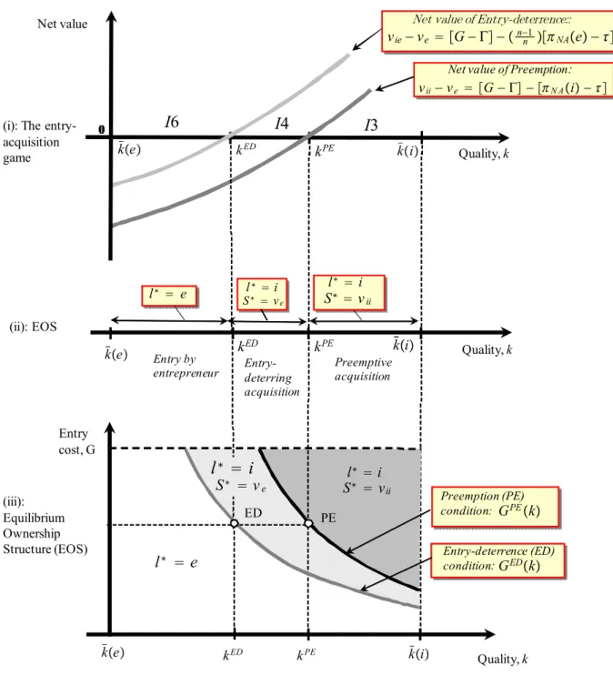
Lemma 3 is proved below and illustrated in Figure 3.1. Figure 3.1(i) solves the acquisition entry game as a function of the quality of the invention, k. When the quality of the invention is lowk∈(¯k(e), kED), the net value for entry deterrence is negative, i.e. an incumbent’s entry deterring valuation is lower than the entrant’s entry value, vie−ve < 0. In this region, the entrepreneur will thus choose commercialization by entry (l∗ =e).
What happens if the quality of the invention increases? Differentiate the net value of entry deterrencevie−ve ink to obtain
v0ie,k−ve,k0 =−¡n−n1¢dπN A(e)
dk >0, (3.3)
where we use v0
k as the notation for the derivative, dv
dk. Thus, the entry-deterring valuation of an incumbent vie increases more than the entrepreneur’s value of entry ve when the quality
Entry by
entrepreneur Entry-deterring acquisition
Preemptive acquisition Net value
(i): The entry-acquisition game
(ii): EOS
l∗ e l∗ i l∗ i
S∗ ve S∗ vii
Net value of Preemption:
Net value of Entry-deterrence::
I
3
I
4
I
6
ED PE (iii): Equilibrium OwnershipStructure (EOS) Entry-deterrence (ED)
condition: Preemption (PE) condition:
l
∗
e
l∗ i S∗ v iil
∗
i
S∗ ve kED kPE k̄e k̄i Quality, k kED kPE k̄e k̄i Quality, k kED kPE k ̄e k̄i Quality, k Entry cost, G vie−ve G−Γ−n−n1NAe− vii−ve G−Γ−N Ai− GEDk GPEkof the invention increases. To see why, note that the first term in vie = πA(i) −τ −Γ−
λ(e) [πN A(e)−τ]increases by the same amount as the first term inve =πE(e)−τ −G, since the acquiring incumbent and the entrepreneur have the same increase in profit from Assumption A1, πA(i) = πE(e). However, since the profit of a non-acquirer πN(e) decreases in k, there is an additional increase in the incumbent’s valuation, thereby implying that v0
ie,k > ve,k0 . Thus, since an incumbent’s net value of entry deterrence vie −ve is increasing in the quality of the invention k, an entry deterring acquisition at the acquisition price S∗ = ve occurs at
k=kED, as shown in Figure 3.1(ii). Other incumbents will not preempt a rival acquisition in the regionk∈[kED, kP E), since the net value of preemption is negative, vii−ve <0. Thus, the entrepreneur will commercialize by sale (l∗=i) at price S∗ =πE(e)−τ−Gin this region.
What if the quality increases even further? Since a higher quality decreases the profit of a non-acquiring incumbent also when there is an incumbent acquisition, the net value of preempting rivals is also increasing in quality. Differentiatingvii−ve inkwe obtain
vii,k0 −v0e,k =−dπN A(i)
dk >0. (3.4)
As shown in Figure 3.1(i), increasing the quality of the invention into the regionk≥kP E will then imply that the net value of preemption is strictly positive, vii−ve >0. This induces a bidding war between incumbents driving the equilibrium sales price above the entry value for the entrepreneur,S∗ =vii=πA(i)−Γ−πN A(i)> ve. The entrepreneur will thus commercialize
by sale (l∗ =i), receiving the sales priceS∗=viiin this region.
Let us now derive additional predictions. Figure 3.1(iii) shows how the equilibrium ownership is jointly determined by the quality of the inventionkand the entry cost G. LetGED(kED)be the entry-deterrence condition (ED-condition) defined fromvie(kED, G) =ve(kED, G), and let
GP E(kP E) be thepreemption condition (PE-condition) defined fromvii(kP E, G) =ve(kP E, G). Solving for Gin each equation, we have:
GED(k) =Γ−¡nn−1¢τ +¡n−n1¢πN A(e), GP E(k) =Γ−τ +πN A(i). (3.5) The loci associated with the takeover condition GED(kED) and the preemption condition
GP E(kP E) are downward-sloping in the k−G space. This follows from the profit of a non-acquirer πN A(l) decreasing in the quality of the invention k, and a lower fixed entry cost G being needed to balance the incumbent’s higher value of obtaining the invention. The equilib-rium ownership structure involves commercialization by entry below the entry deterrence locus
GED(k), indicated as l∗ =e. Entry deterring acquisitions occur for combinations of k and G
between the takeover locusGED(k) and the preemption locusGP E(k), indicated as l∗ =i and
S∗ = ve. Preemptive acquisitions occur above the preemption locus GP E(k), as indicated by
l∗ =iandS∗=vii. From (3.5), we also note that increases in transaction costsΓshift the entry deterrence locusGED(k)and the preemption locus upwards in Figure 3.1(iii), thus reducing the region where commercialization by sale occurs, whereas increasing the fixed operating cost τ
has the opposing effect.
Thus, we can state the following result:
sale to incumbents and entering the market, an entrepreneur will then prefer sale when (i) the quality of the invention k is high, (ii) when entry costs G are high, (iii) when operating fixed costsτ are high, and (iv) when the transaction costs associated with a saleΓ are low.
3.2. Non-market-structure neutral entry
We will now relax Assumption A1. Let usfirst examine the case when the quality of the invention is so low that no incumbent is forced out of the market post-entry, i.e. N(i) =n < N(e) =n+1, i.e. we assume
Assumption A2 Non-neutral-entry without exit: k∈(0,¯k(i)).
From (2.5), (2.6), and 2.7), (3.1) now becomes:
vil−ve= [πA(i)−Γ−πE(e) +G]−[πN A(l)−τ], l={e, i}. (3.6) Differentiating (3.6) ink, we obtain: vie,k0 −ve,k0 = ∙ dπA(i) dk − dπE(e) dk ¸ −dπN Adk(l) l={e, i}. (3.7)
The main difference from the above analysis is that the effects on the entrant and the acquirer of an increase in quality now differ, i.e. dπA(i)
dk 6= dπE(e)
dk , so we cannot in general sign the invention transfer effect. However, in many oligopoly models, including the Linear Cournot model, dπA(i)
dk > dπE(e)
dk holds, i.e. a larger acquirer (as compared to the entrant) would have more to gain from increased quality due to larger sales, andvie,k0 −v0e,k >0. As can be shown, we can state the following result7:
Lemma 4. Proposition 3 is fulfilled in the LC-model fork∈(0,¯k(i)).
What would then happen if we allowed for such drastic inventions that more than one incumbent firm would exit the market? Let πm denote the monopoly profit. Then, make the following assumption
Assumption A3 k∈(¯k(i), kmax], where πA(i) =πE(e) =πm fork=kmax. Under Assumption A3, (3.6) becomes
vil−ve = [πA(i)−Γ−πE(e) +G]−λ(l)[πN A(l)−τ], l={e, i}´. (3.8) To see that a higher quality of the invention is conducive to innovation also in this setting, suppose thatvil−ve >0holds for some k >k¯(i). Note that thefirst term in (3.8) would remain positive, while the second term would decrease in the quality of the invention. The second term could increase discretely when the exit of an incumbent takes place (sinceπN Aincreases). Such discrete changes would nevertheless decrease in size as non-acquirers become smaller. While there would be situations where small changes in quality imply that we move from an equilibrium
of commercialization by sale to one with commercialization by entry, commercialization by sale will prevail when the quality of the invention becomes sufficiently high.8
4. Why preemptive acquisitions may promote the process of creative
destruc-tion
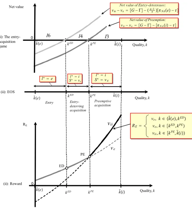
In this section, we will show that preemptive acquisition will accelerate the process of cre-ative destruction. To illustrate this, first assume that Assumption A1 holds. The following proposition concerning research incentives for the entrepreneur is then immediate:
Proposition 2. Assume that Assumption A1 holds, then ρ∗(i) > ρ∗(e) for k ∈ [kP E,¯k(i)). That is, entrepreneurs with high-quality projects will be substantially more likely to succeed with an invention under commercialization by sale as compared to commercialization by entry. The proposition is proved in Figure 4.1 where, for convenience, Figure 4.1(i) derives the equilibrium commercialization strategy for the entrepreneur and Figure 4.1(ii) depicts the re-ward of the entrepreneur RE(l) as a function of the quality of the invention k. When quality is low k ∈ (¯k(e)), kED), commercialization by entry occurs and the reward is R
E(e) = ve =
πE(e)−τ−Gfor the entrepreneur. From Definition 1,RE(e)is increasing in quality and from Lemma 2, the research incentives are increased. The same holds if an entry deterring acquisition occurs in region k∈[kED, kP E) sinceR
E(i) =S∗ =ve.
However, at an even higher qualityk≥kP E,preemptive acquisitions occur, and the bidding competition between incumbents over the benefits as an acquirer — as well as over avoiding a weak position as a non-acquirer — drives the reward for commercialization by sale to be strictly higher than the reward for commercialization by entry, RE(i) = vii > ve = RE(e). But then, since the research effort and hence, the likelihood of a successful innovation ρ∗(l), is increasing in the reward RE(l) from Lemma 2, it directly follows that the probability of a successful invention will be higher under commercialization by sale. This is illustrated in Figure 4.1(iii) which shows that preemptive incumbent acquisitions of entrepreneurial inventions can be productive by substantially increasing the research incentives for entrepreneurs.
More generally, we may also note that Lemma 1 and Lemma 2 imply that preemptive in-cumbent acquisitions will always increase the reward to research for entrepreneurs substantially, sinceS∗ =vii> ve and hence ρ∗(i) > ρ∗(e) will hold for any of the inequalities I1, I2 or I3 in table 2.1.
4.1. Preemptive acquisitions and welfare
Let us first examine how incumbent acquisitions of entrepreneurial inventions affect consumer welfare. To this end, we compare a Non-discriminatory (ND) policy (where incumbent acquisi-tions of entrepreneurial firms are allowed) to a Discriminatory (D) policy (which prohibits the acquisitions of small innovativefirms). Consider a stage 0 where a government chooses between the two polices. Formally, letΓ¯ be defined fromvie(·,Γ¯) = 0. In the ND-policy,Γ<Γ¯, whereas in the D-policy,Γ>Γ¯. This is a highly stylized comparison, but it can be seen as a simple way of
8
Entry Entry-deterring acquisition Preemptive acquisition Net value
(i): The entry-acquisition game (ii): EOS l∗ e l∗ i l ∗ i S∗ ve S∗ vii
I
3
I4 I6 kED kPE k̄e k̄i Quality, k kED kPE k̄e k̄i Quality, k (ii): Reward kED kPE k̄e k̄i Quality, k ED PE REv
ii RE ve, k ∈ k̄e,kED ve,k∈ kED,kPE vii,k ∈ kPE,k̄i 0 0Net value of Preemption:
Net value of Entry-deterrence::
vie−ve G−Γ−n−n1NAe−
vii−ve G−Γ−N Ai−
v
ecapturing the effects of substantial changes of transaction costs for acquisitions due to changes in policies that might block or increase the cost of acquisitions of small innovative firms.9 10 The change in transaction costs could also stem from technological and institutional changes.
Assume that, all else equal, consumers benefit from a higher quality of the innovation and from more firms being present in the market. Let the consumer surplus under ownership l be denoted CS(l), and let CS(0)denote the consumer surplus when the entrepreneur fails. From Lemma 1, we have: CSN D−D= ⎧ ⎪ ⎨ ⎪ ⎩ 0, for I5,I6 ρ(e) [CS(i))−CS(e)]≤0, for I4 ρ(i) [CS(i)−CS(0)]−ρ(e) [CS(e)−CS(0)] for I1-I3, (4.1)
noting thatρ(e) =ρ(i) under I4 in Table 2.1.
If incumbent acquisitions are driven by entry deterrence motives, consumers will be better off
from the Discriminatory policy, as shown byCSN D−D ≤0 under I4. However, the differential
CSN D−Din (4.1) also reveals that consumers may prefer the ND-policy when inventions are sold under bidding competition, since a successful invention is more likely, i.e. since ρ∗E(i)> ρ∗E(e)
under inequalities I1-I3 in Table 2.1. Since a higher quality of the invention will induce bidding competition among incumbents, this suggests that consumers may prefer the ND-policy when potential innovations are of high quality. This is shown by the following proposition:
Proposition 3. If inventions have a sufficiently high quality k > ¯k(e), consumers will prefer the ND-policy over the D-policy,CSN D−D>0.
Proof. First, note thatk >k¯(e)implies thatn(i) =n(e)from Definitions 2 and 3 and, hence,
CS(i) = CS(e), since no market power effect then arises from the acquisition. The higher entrepreneurial research effort under the ND policy ρ∗E(i) > ρE∗(e) then implies CSN D−D >0
fork >¯k(e).
Thus, preemptive incumbents’ acquisitions may benefit consumers by giving entrepreneurs stronger incentives to succeed with high-quality inventions. For inventions of lower quality
k <¯k(e), the market power effect may dominate the higher probability of a successful invention. Let us end with a brief remark on how the total surplus is affected by policy. It directly follows that the entrepreneur gains from the ND-policy, since the bidding competition may give premium reward to successful invention.11 What about incumbents? Let πN(0) denote the profit for incumbents absent the invention. From Lemma 1, we can then derive the difference in expected incumbents’ profits from the two polices:
9 Examples are a restrictive merger policy in R&D industries, or tax policies concerning the sale of innovativefirms.
1 0
An alternative policy with qualitatively the same effect would be a reduction in the cost of entry. 1 1
To see this, define the reduced-form entrepreneurial profit asΠE(l) =ρ∗(l)RE(l)−y(ρ∗(l)). Since
RN D
E (l) =RDE =ve under I4, I5 or I6 in Table 2.1, whereasRN DE (l) =S∗ =vii > RDE =ve,ΠN DE (l)≥
P SN D−D= ⎧ ⎪ ⎪ ⎪ ⎪ ⎪ ⎪ ⎪ ⎪ ⎪ ⎨ ⎪ ⎪ ⎪ ⎪ ⎪ ⎪ ⎪ ⎪ ⎪ ⎩ 0, for I5,I6 ρ∗(e) ⎧ ⎨ ⎩n{|λ(i) [πN(i)−τ]−{zλ(e) [πN(e)−τ}] >0 }+v| {z }ii−ve <0 ⎫ ⎬ ⎭, for I4 ⎧ ⎨ ⎩ρ|∗(e){z−ρ∗(i}) <0 ⎫ ⎬ ⎭πN(0) +n ⎧ ⎨ ⎩ρ|∗(i)λ(i) [πN(i)−τ]−{zρ∗(e)λ(e) [πN(e)−τ}] >0 ⎫ ⎬ ⎭, I1-I3. (4.2) Expression (4.2) reveals that which policy incumbents prefer is ambiguous. For instance, under preemptive acquisitions, when one of the inequalities I1-I3 in Table 2.1 is fulfilled, there is a larger expected loss of ex ante rents due to higher research efforts under the ND policy (as shown by the first term in the third line). But, given that the entrepreneur succeeds, which occurs with probabilityρ∗(l), the expected profit is higher under the ND-policy since incumbents either gain from a higher concentration by avoiding entry or by avoiding a less uncertain position as a non-acquirer (as shown by the second term in the third line).
5. Empirical analysis
We now turn to the empirical analysis. We first derive a probit model from the entrepreneur’s decision on the mode of commercialization in stage 2, which is then estimated on a unique dataset on patents granted to Swedish small firms and individual inventors.
5.1. Deriving an estimation equation for the mode of commercialization
To identify if the model is consistent with the data and, in particular, with preemptive acqui-sitions, we will estimate the entrepreneur’s choice of commercialization in Stage 2. Then, let
Re,m be the reward for an entrepreneurechoosing commercialization mode m= (Sale, Entry), consisting of the reward RE,m(ke, τe,Γe, Ge) given from Lemma 1 and a stochastic termεe,m, i.e.
Re,m=RE,m(ke, τe,Γe, Ge) +εe,m, m= (Sale, Entry), (5.1) whereεe,mcaptures idiosyncractic factors affecting entrepreneure’s choice of commercialization not captured in the theory. In what follows, we assume that the entrepreneur knowsRe,m and its components, while the error term is unknown to the econometrician.
To proceed, we linearize RE,m(ke, τe,Γe, Ge) in its components assuming that Assumption A1 is fulfilled. Noting thatRE,Entry(ke, τe,Γe, Ge) =veunder entry, whereasRE,Sale(ke, τe,Γe, Ge) =
S∗ under sale, we have:
RE,Entry(ke, τe,Γe, Ge)≈α0+αk (+) ke+αG (−) Ge+αT (0) Γe+ατ (−) τe=x0eα (5.2) RE,Sale(ke, τe,Γe, Ge)≈β0+βk (+) ke+βG (?) Ge+βT (?) Γe+βτ (?) τe=x0eβ. (5.3)
To identify preemptive acquisitions in the data, we proceed as follows. First, note that the signs in (5.2) directly follow from (2.7) and Definition 1. In (5.3), we note that when an
entry-deterring acquisition takes place, S∗ = ve, and β=α. In contrast, when an acquisition is preemptive, the bidding competition between incumbents drives up the the acquisition price to S∗ =vii > ve, which implies β6=α. To see this, first note that (3.4) implies βk−αk >0, which is illustrated in Figure 4.1(ii) where the reward-locus under sale and bidding competition,
RE =vii,being steeper in qualitykthan the corresponding reward under innovation for entry,
RE = ve. Then, note that (2.5) and (2.7) directly imply βG −αG > 0, βΓ−αΓ < 0 and
βτ −ατ >0.
Using (5.1)-(5.3), we can now write down the probability that the entrepreneur will choose commercialization by sale as:
Prob[Salee]=Prob[Re,Sale > Re,Entry]=Prob[εe,Entry−εe,Sale <x0e(β−α)]
=Prob[εe<x0eγ]= Z x0
eγ
−∞
f(εe)dεe=F(X0eγ), (5.4)
where γ=β−α and f(εe) is the density of the error term, εe = εe,Entry −εe,Sale. If εe,m is distributed according to the Gumbel distribution, then εe will be distributed according to the logistic distribution and F(x0eγ) = Λ(x0eγ), where Λ(·) is the cumulative density function of the logistic distribution. When εe,m are mean-zero normally distributed, εe will also be normally distributed and F(x0eγ) = Φ(x0eγ), where Φ(·) is the cumulative density function of the normal distribution. In either case, parameters γ can be estimated by maximizing the likelihood function:
L=Π eF(x
0
eγ)meF(1−x0eγ)1−me, (5.5) where me = 1when commercialization by sale is chosen and me = 0when commercialization by entry is chosen.
Thus, using the fact that γ=β−α in (5.4), we can derive a testable hypothesis on the nature of incumbent acquisitions from our proposed model. We have the following proposition:
Proposition 4. Suppose that Assumption A1 holds. Then:
(i) If commercialization by sale takes place by entry-deterring acquisitions at S∗=ve,then γ=0, or equivalently,β=α.
(ii) If commercialization by sale takes place by preemptive acquisitions at S∗ = vii > ve, γ6=0, or equivalently, β6=α. More specifically, γk = βk −αk > 0, γG = βG −αG > 0,
γΓ =βΓ−αΓ<0and γτ =βτ −ατ >0.
Before proceeding, we make a number of remarks on the generality of Proposition 4.
Assumption A1: Proposition 4 does not require that entrepreneurial entry is "market neu-tral". This follows directly from table 2.1 (which applies also in situations where Assumptions A2 and A3 are fulfilled) where we again note that preemptive bidding competition implies
S∗ =vii> ve.
Linearization of RE,m(·): Proposition 4 is based on a linearization of RE,m(·) in (5.1). Ambiguities may then arise in Proposition 4(ii), since theory gives no guidance to whether
RE,m(·)is concave or convex ink. Note however that (2.5) and (2.7) implies thatRE,mis linear inGand T. Then, simultaneouslyfinding thatγk>0,γG >0,γΓ <0and γτ >0can only be only consistent with preemptive bidding competition between incumbents generating the sales priceS∗ =vii> ve.
Proposition 1: Propositions 4(i) and (ii) are, respectively, sufficient conditions for the theory in Proposition 1. That is, in terms of Figure 4.1(ii), evidence for Proposition 4(ii) must imply that incumbent acquisitions take place in the dark-shaded area where acquisitions are preemp-tive at S∗ =vii, whereas evidence for Proposition 4(i) would correspond to acquisitions taking place in the light-shaded area where acquisitions are entry-deterring atS∗ =ve. Rejecting our proposed theory on the mode of commercialization of entrepreneurial inventions thus requires γ6=0 as well as a reversal of all signs in Proposition 4(ii).
Endogenous quality: Proposition 4 also holds in a setting where the entrepreneur chooses the level of qualitykin stage 1 (rather than affecting the probability of discovering an invention of a given quality). To see this, let C(k) be a strictly convex development cost. Assuming that Assumption A1 is fulfilled, (2.5) and (2.7) then imply kSale = arg maxk[vii−C(k)] >
kEntry= arg max
k[ve−C(k)]. Thus, our theory would also predict that entrepreneurs choosing commercialization by sale will have a stronger incentive to develop inventions to higher quality. This suggests a potential endogeniety problem in (5.4). However, note that the entrepreneur will choose the mode of commercialization to maximize RE,m(·) in (5.1) in stage 2, where the quality of the innovation k is given from stage 1. It then follows that we can use Proposition 4 to identify preemptive acquisitions, irrespective of whether the quality of an innovation is exogenously given for the entrepreneur, or if the the entrepreneur could affect the quality prior to commercialization.
Asymmetric incumbents: We should finally note that identifying preemptive acquisitions through Proposition 4(ii) does not require symmetric incumbents. This follows from the fact that with a market with asymmetric incumbents, the sales price would either be the reservation price ve or the valuation for the incumbent with the second highest valuation, vii2. If the invention generates negative externalities through the product market for the firm with the second highest valuation, and if these externalities are sufficiently strong, the acquisition price will once more be bid up aboveve.
5.2. Data
To estimate (5.4), we will use a dataset on patents granted to small firms (less than 200 em-ployees) and individual inventors. The dataset is based on a survey of Swedish patents granted in 1998.12 In that year, 1082 patents were granted to Swedish small firms and individuals.13
1 2 A further description of the data can be found at http://www.ifn.se/web/Databases_9.aspx and in Svensson (2007).
1 3
In 1998, 2760 patents were granted in Sweden. 776 of these were granted to foreign firms, 902 to large Swedishfirms with more than 1000 employees, and 1082 to Swedish individuals andfirms with less than 1000 employees. In a pilot survey carried out in 2002, it turned out that large Swedishfirms refused
Information about inventors, applying firms, their addresses and the application date for each patent was obtained from the Swedish Patent and Registration Office (PRV). Thereafter, a questionnaire was sent out to the inventors of the patents in 2004.14 The inventors were asked where the invention was created, if and when the invention had been commercialized, which kind of commercialization mode was chosen, type of financing, etc. 867 out of 1082 inventors filled out and returned the questionnaire, i.e., the response rate was 80 percent.15
From the theory, we are interested in those patents where the inventors can decide themselves whether to commercialize the patent. Therefore, we will only consider 624 patents where the inventors have some ownership. 364 out of these 624 patents were commercialized, that is, the holder received income from the patent.16 Among the 364 commercialized patents, 91 patents were commercialized by selling or licensing the patent, and 273 patents were commercialized by entry and own commercialization. Since the mode of commercialization is chosen from maximizing the reward or income from an innovation,RE in (5.1), we will use commercialized patents when estimating (5.4). The potential econometric problems arising from 260 out of 624 patents in the sample not being commercialized will be dealt with in Section 5.4.
5.2.1. Dependent variable: mode of commercialization
As the dependent variable in (5.4), we thus define a binary variableSaletaking the value of one if the patent was sold or licensed to another firm, and zero if the patent was commercialized internally by the inventor. Note that a sale of an invention and an exclusive licence of an invention are equivalent in our theory. Since the licensing contracts are almost only exclusive in the data, we treat licence contracts and sales as symmetric in the empirical analysis.17 to provide information on individual patents. Furthermore, it is impossible to persuade foreignfirms to fill out questionnaires about patents. Thesefirms are almost always large multinationalsfirms
1 4 Each patent always has at least one inventor and often an applying firm. The inventors or the applying firm can be the owner of the patent, but the inventors can also indirectly be owners of the patent, via the applying firm. Sometimes, the inventors are only employed in the applying firm which owns the patent. If the patent had several inventors, the questionnaire was sent to one inventor only.
1 5 The falling off was not systematic. The falling off was due to 10% of the inventors having old addresses, 5% having correct addresses but we did not get any contact with the inventors and 5% refusing to reply. The only information we have about the non-respondents is the IPC-class of the patent and the region of the inventors. For these variables, there was no systematic difference between respondents and non-respondents.
1 6 The commercialization rate for our sample is 58 percent. This rate should be compared to the few available studies which have measured the commercialization of patents: 47 percent for American patents found by Morgan et al. (2001) and 55 percent in the studies surveyed by Griliches (1990). The higher commercialization rate in the present study is explained by the fact that only patents directly or indirectly owned by the inventors are included — large (multinational)firms have a much larger number of defensive patents. Griliches (1990) confirms this view and reports that the commercialization rate is 71 percent for smallfirms and inventors.
1 7 In many cases, when the invention to a large extent consists of indivisible assets in terms of capital or human capital, exclusive licences are self evident. However, in some situations, several buyers might hold a licence to utilize the innovations. Kamien and Tauman (1986) and Katz and Shapiro (1986) show that there exists an equilibrium where some potential buyers are left without a licence also when multi-firm licensing is an option. Thus, exclusivity is also a possible outcome in situations where entrepreneurs can
5.2.2. Explanatory variables
The explanatory variables used in estimating (5.4) and their expected signs are given in Table 5.1.
The quality of an invention,k To measure the quality of an inventionk, we use the number of forward citations (excluding self-citations) that a patent received from the application date until November 2007. With patents having different application years, the length of the time periods they can be cited differs. Therefore, in the estimations, we adjust our citation variables so that they measure the number of forward citations in a five-year period.18
Forward citations are seen as the most important quality indicator of patents in the lit-erature (Harhoff et al., 1999; Lanjouw and Schankerman, 1999; Hall et al., 2005). We divide the forward citation variable into two groups: (i) forward citations where the cited and cit-ing patents have at least one common technology class at the four-digit ISIC-level, denoted as
W_CIT; and (ii) forward citations where they have no common technology class at the four
-digit ISIC-level, denoted as B_CIT. Proposition 4(ii) implies that if incumbent acquisitions are driven by preemptive motives, we would expectγk=βk−αk>0. The quality of the inven-tion kdriving incumbents’ preemptive motives should then be reflected in obtaining a positive estimate onW_CIT rather than forB_CIT, since the former should indicate how frequently competitors cite the patent; competitors should apply for similar patents, and frequent citations from competitors should therefore indicate high quality within the industry.19
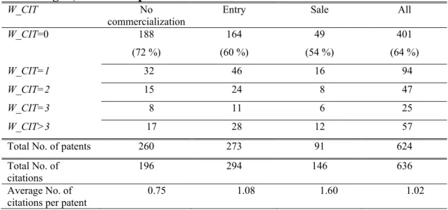
The 624 patents in the sample together have 636 forward citations within technologies and 79 between technologies. In table 5.2, the relationship between commercialization mode and forward citations within technologies (W_CIT) is shown. Most patents (64 percent) have no forward citations at all, and cited patents seldom have more than three citations. Among non-commercialized patents, only 28 percent are cited, whereas 40 and 46 percent of the entry and sale patents are cited. In line with the theory, we note that patents which are commercialized through sale have a higher average number of forward citations than patents which are commercialized through entry. Patents which are not commercialized have the lowest average.
A potential concern with our quality measure is endogeneity, since forward citations in general occur after the patents have been commercialized. Forward citations are registered by administrators at the national patent offices, who can be seen as independent actors; they are hardly affected by any commercialization decision. However, the fact that commercialization by sale or entry has occurred may make competitors apply for related patents which, in turn,
sell several licences and our set-up is also valid in situations wherefirms have the option to sell a licence to more than onefirm.
1 8 Here, we follow the approach of Trajtenberg (1990) and weight the number of received patent citations by linear time trend.
1 9
It is also competitors that should be interested in acquiring or licensing the patent. For example, a high-quality drug patent, which largely affects competitors’ profitflows, should have more citations from future patents of drugs than from patents of semi-conductors, say. The cost for competitors should then come from limits in their own patents or through increased costs of generating competitive new patentable innovations.
cite the original patent. If this is true, forward citations would increase for around 2-5 years (the time it should take to develop a new invention and file a patent) after sale or entry has occurred. Table 5.3 shows the number of forward citations that patents have received during the years before and after application, entry and sale occurred. If it is assumed that a competitor cannot apply for a new patent within two years after entry or sale occurs, it seems as if neither entry nor sale affects forward citations.20 To deal with this potential endogeneity problem, we transform the citation variables W_CIT and B_CIT into binary variables, D_W_CIT and
D_B_CIT indicating whether a patent received a citation. Such citation dummy variables should be less sensible to the endogeneity problem than the original ones.
Entry costs, G To measure the costs of commercialization under entry G, we use additive dummies for different firm sizes. Firms which already have marketing, manufacturing and financial resources in-house should have lower costs of entering the market for a new product,
G. We define the variable SM ALL taking on the value of 1 for firms with 11-200 employees, and 0 otherwise, whereas M ICRO equals 1 for micro companies with 2-10 employees, and 0 otherwise. Entrepreneurialfirms with either of these characteristics should face lower entry costs than the reference group of inventors without any employees. Since largerfirms should facelower entry costsG, the bidding competition among incumbents for entrepreneurial inventions implies thatγG=βG−αG>0and Proposition 4(ii) thus impliesγGM ic ro <0andγGSmall <0.In Table 5.4, the commercialization mode rates are shown for different firm sizes. Commercialization by sale is more frequent the smaller is firm size, whereas entry is more frequent the larger is the firm, which is consistent with Proposition 4(ii).
Transaction costs, Γ We use the variable PVC measuring the percentage of the R&D-stage that wasfinanced by private venture capitalists or business angles as a measure of transaction costs Γ. Gans et al. (2002) find evidence that the involvement of private venture capitalists increased the probability of commercialization by sale, arguing that such agents have networks with firms, thereby decreasing the search and transaction costs associated withfinding an ex-ternal buyer. Thus, if a stronger participation of venture capitalists in the commercialization process reduces the transaction costsΓ, it follows from Proposition 4 that preemptive acquisi-tions by incumbents of entrepreneurial innovaacquisi-tions implies γΓP V C >0.
Operational fixed costs, τ We do not have any measure offixed operation costs,τ. Instead we use additive dummies (fixed effects) for technologies and regions as well as a trend variable for the application year, broadly controlling for unobservable technology-, region- and time-specific factors. Patents are divided into technology groups based on the patents’ main IPC-Class according to Breschi et al. (2004). The data is also divided into six different regions. Five additive dummies are included for these six groups in the estimations. A trend variable
AP P LY is also included, measuring the application year.
2 0 Note also that most entries occur about 1-3 years after the patent application (see Table 5.3), which explains the low value of 23 citations in thefirst year after entry.
5.3. Results
The results of estimating the probit model (5.4) are shown in table 5.5. Let us first examine if these results are consistent with preemptive acquisitions by incumbents. We start with Model A containing the core variables from the theory, W_CIT, P V C, SM ALL and M ICRO, as well as fixed effects for technologies and regions. The Wald test on the core variables shows thatγ=0in (5.4) or, equivalently,β=αis rejected. This is also the case in the Wald test on the full specification of Model A.
Next, we turn to individual estimates. A higher quality of the invention as measured by more forward citations (W_CIT) increases the probability of an invention being commercialized by a sale to incumbents. On the other hand, presence in the market as measured by either being a small or a micro firm (SM ALL and M ICRO) decreases the probability of a sale. All these variables are statistically significant. The estimated coefficient of P V C has the correct sign, but is not significant. Since we can rejectγ =0 and since the coefficients of the core variables are consistent with γk =βk−αk >0, γΓ=βΓ−αΓ <0 and γG =βG−αG >0, Proposition 4(ii) implies that the estimates identify incumbent acquisition as being preemptive in nature.21 In Models B and C we add between citations B_CIT and the application year AP P LY, without qualitative changes in results. The Wald tests and individual estimates are again consistent with the Proposition 4(ii). Calculating marginal effects shows that if a patent receives one more forward citation during afive-year period, the probability of sale increases by about five percentage points in Models A-C. If the inventor has a smallfirm as compared to the case where she has nofirm, the probability of sale decreases by around 20 percentage points.
Due to the potential endogeneity problem our citation variable and the distribution of forward citations being skewed to the right, we reestimate (5.4) with the citation dummies
D_W_CIT and D_B_CIT, indicating whether a patent received a citation. These results are shown in table 5.6. The Wald tests again reject γ=0, whereas the results for individual estimates are consistent with γk = βk−αk >0, γΓ = βΓ−αΓ < 0 and γG = βG−αG > 0. Once more, the results are thus consistent with Proposition 4(ii), albeit some estimates are less precise.
As a second check, we also re-estimated table 5.5 with OLS and logit specifications without finding any qualitative changes in the results. The results were also unaffected by adding a number of control variables such as the share of ownership in the entrepreneurial firms held by the inventor, notwithstanding if the inventor had complementary patents or more patents, individual characteristic of the inventor such a sex or ethnicity, or whether the patent was applied in research at a university.
5.4. Extension: the decision to commercialize
The theory presented makes the implicit assumption that all patents are commercialized. In contrast, about 40 % of the patents in the sample were not commercialized. Among the non-commercialized patents, 163 expired before the end of the data collection in 2005, while 97
2 1
The exception isγτ=βτ−ατ = 0since we have no direct measure of operatingfixed costs,τ .The
impact of τ is indirectly estimated through the Wald test onγ =β−α= 0, where the impact of τ is (imprecisely) accounted for in the technology and region-fixed effects.
patents remained active in 2005 and may, in principle, have been commercialized after the observation period.22
We investigate this data problem in three ways. First, we re-estimate the probit model in (5.4) with a sample selection correction, pooling both types of non-commercialized patents. Second, we estimate a multinomial logit model which is based on an extension of the theory to include the decision to not commercialize an invention. The latter model uses the information from non-commercialized patents where the inventors actively dropped their patent. Finally, we employ a duration analysis. This method takes account of the timing decision and controls for the fact that some patents may have been commercialized after the sample period.
5.4.1. Selection bias
Since the group of commercialized patents may not be a random sample of patents, but may have rather specific characteristics which led to them to be commercialized, there is a potential sample selection problem in 5.4.
To control for this, we also model the probability of commercialization
ce=I[θ0+θzze+θ0Xe+ue >0], (5.6) where ce = 1 if commercialization is chosen and ce = 0 otherwise. ze is a variable which only affects the choice to commercialize but not the mode of commercialization. The variablezecan be considered as a variable identifying draws of low-quality inventions, or inventions associated with high costs for commercialization, which would imply RE,m(·) +εe,m < 0 in (5.1). The vectorXe contains the same explanatory variables as those included in the probit model (5.4). How may selection bias affect the estimates of γ in (5.4)? Suppose that ue and εe in (5.4) and (5.6) contain an unobserved quality of the patent. From Definition 1, patents with a high unobserved quality will tend to be commercialized. But then, since ue and εe are positively correlated (due to the unobserved quality), commercialized patents with high unobserved quality will tend to be sold to incumbents by Lemma 3. This selection mechanism may potentially generate an upward bias on the estimate ofγ=β−αin (5.4).
Assuming that the error terms ue and εe are correlated according to a bivariate standard normal distribution with correlationρ, (5.4) and (5.6) can be jointly estimated with maximum likelihood to obtain an estimate of γ =β−α to test Proposition 4.23 Svensson (2007) shows that government-financed inventions are less likely to be commercialized, arguing that inventions of inferior quality seek government support for commercialization and that the government loan terms discourage commercialization.
In table 5.7, we report the selection model using the full sample of 624 observations. Using the percentage of the R&D-stage financed by government (GOV) as the identifying variable
ze, we note that the results in the second-stage sale equation do not change qualitatively in relation to the corresponding probit specifications in table 5.5 and results are again consistent with Proposition 4(ii). Inspecting individual estimates, we note thatW_CIT is still significant
2 2
This is less likely, however. In Svensson (2007), it was shown that the probability is very low that the 97 non-commercialized patents, which are still alive, will ever be commercialized.
at the five-percent level. If a patent receives one more forward citation during a five-year period, the probability of sale increases by 4-5 percentage points in Models A-C. While thefirst stage identifies the commercialization decision through the government financing variable, the correlation between error terms ue and εe is not significant.24
5.4.2. Identification with multinomial logit
The probit model with selection suggests that the error terms in the commercialization decision and the choice of type of commercialization are not correlated. Assuming this to be the case, we can formally integrate the commercialization decision into the theory, thus providing additional information for identification.
To see this, let Re,N o(k, τ ,Γ, G) =RE,N o(ke, τe,Γe, Ge) +εe,N o be the reward for ”No com-mercialization”. By definition, RE,N o(ke, τe,Γe, Ge) = 0 which can be (trivially) linearized in its arguments: Re,N o(ke, τe, Te, Ge) =ψ0 (0) +ψk (0) kr+ψF (0) Fr+ψT (0) Γr=x0eψ. (5.7)
Then, letm, l= (Sale, Entry, N o). The probability that the entrepreneur will choose commer-cialization mode m instead of commercialization mode l is then Prob[me]=Prob[Re,m > Re,l] ∀m6=l, or Prob[me]=Prob[εe,l−εe,m< RE,m(k, τ ,Γ, G)−RE,l(k, τ ,Γ, G)]∀m 6=l. Assuming thatεe,mis distributed according to the Gumbel distribution,εe=εe,m−εe,lwill be distributed according to the logistic distribution. Under the assumption thatεe,N o,εe,Sale and εe,Entry are not correlated, this gives rise to a multinomial logit model, where:
Prob[Salee] =
ex0eβ
ex0eβ+ex0eα+ex0eψ, Prob[Entrye] =
ex0eα
ex0eβ+exe0α+ex0eψ. (5.8)
Maximum Likelihood can now be used to estimate γSale=β−ψ and γEntry =α−ψ, where ψ =0 from (5.7) identifies vectors β andαfrom (5.2) and (5.3).
In table 5.8, we show the results from estimating (5.8) for the 364 patents which are com-mercialized (by Sale or Entry) and the 163 patents where we know that the holder actively chose not to commercialize (i.e. the patent expired without any income for the holder).25 Given the identifying assumption of ψ = 0, Wald tests show that β = 0,α = 0 and β = α can all be rejected. Moreover, the parameter estimates and Wald tests on the citation variable
W_CIT and, in particular, the citation dummy D_W_CIT indicate evidence of αk > 0 in (5.2), βk>0 in (5.3) andβk> αk.Calculating marginal effects shows that if a patent receives one more forward citation during a five-year period, the probability of sale increases by 3.8 percentage points, entry increases by 2.6 percentage points and no commercialization decreases by 6.4 percentage points. From the estimates of SM ALLand M ICRO, we also note that the
2 4 We also re-estimated table 5.6 with the citation binary variables, D_W_CIT and D_B_CIT without a qualitative change in the results.
2 5
We omit the remaining 97 observations since we do not know the commercialization decision for these patents. This right-censoring problem is taken into account in the next section which uses a duration analysis.