A Transaction-Level Tool for Predicting TCP Performance and for Network
Engineering
Jean Walrand
Department of Electrical Engineering and Computer Sciences
University of California at Berkeley
Berkeley, CA 94720
Abstract
Traditional traffic engineering for communication net-works assumes that the sources generate traffic with known statistics. Using simulation and/or analysis, one then stud-ies the quality of service that the network offers to these traffic streams.
However, most of the traffic in the Internet is TCP-based. TCP, the Transmission Control Protocol, regulates the de-livery of packets to correct errors and avoid saturating the destination of the packets or routers inside the network. Ac-cordingly, the traffic that a TCP source generates is not specified a priori. Instead, this traffic depends in an es-sential way on the QoS that the network provides.
In this paper, we propose a simple model and we use it to predict the QoS that a network provides to TCP connec-tions. The tool can compute the probability that each con-nection gets at least some given throughput. Conversely, the tool can be used to design the network to ensure that every connection gets a given throughput with a specified proba-bility. The tool incorporates uncertainties about the load on the network and about the model.
1
Introduction
Network engineering tools for the Internet include measure-ment systems, simulation packages, and analytical methods and results. The tools should provide guidelines on how to expand network capacity, design new networks, introduce classes of service, provision support for voice over IP (the Internet Protocol), estimate reliability, and assess the poten-tial of new technologies.
Existing tools have serious limitations. Measurement systems are useful to evaluate the performance measures of an existing network. As such, these systems can be used to identify bottlenecks and to detect when the network must
be upgraded. The measurement systems can also help track the evolution of network traffic and performance. However, it is difficult to extract more general conclusions from mea-surements. Without additional tools, measurements cannot predict what would happen after a modification of the net-work or of its load.
Simulations do not scale and always rely on fairly arbi-trary models. Often, simulation packages provide an illu-sion of accuracy and sophistication. Usually, they provided detailed results based on arbitrary assumptions. Sometimes, the simulations provide confidence intervals around esti-mated values. However, these confidence intervals assume that the assumptions are exact. Of course, simulations are very useful, necessary in fact, to verify that protocols are correct and to discover how to improve systems. Using sim-ulations (e.g., [3]), you can verify that TCP is biased in favor of connections with a shorter round-trip time and that RED (Random Early Detection) and ECN (Explicit Congestion Notification, see [2]) help correct that bias and improve the utilization of the network links. You can also verify that WFQ (Weighted Fair Queuing, see [1]) helps protect classes of traffic against each other. There are many examples of useful applications of simulations in network engineering. However, simulations do not scale to a reasonable size. For instance, NS (see [4]), the network simulator developed at the Lawrence Berkeley National Laboratory, is one of the best simulation tool for TCP/IP networks. However, try us-ing NS to simulate 100 TCP connections that go through a network with three nodes. You will discover that simula-tions are painfully slow. Moreover, the simulation results are difficult to trust. You would need to make a huge num-ber of simulation experiments while varying the assump-tions to get a sense of likely performance measures. The same comments can be made about commercial packages that usually focus more on giving the user a nice graphical interface than on simulation efficiency. See [5] for a discus-sion of the limitations of simulations of the Internet.
Analysis has had a disappointingly modest impact on network design. Although an impressive body of work is available on network performance evaluation, the fraction of that work that has influenced network engineering is very minute. This lack of impact is explained by the limitations of analysis. Exact analysis is tractable only for overly sim-plified models; approximate analysis provides results that may be difficult to trust. Most often, analysis provides an important qualitative insight and explains critical aspects of network operations. Although this insight can guide the de-velopment of new protocols, it is not sufficient to size a net-work and help its design.
Thus, network engineering tools are sorely needed but existing tools are inadequate. How can more useful tools be developed? Useful tools should have the following charac-teristics:
1. Robust: The tools should provide trustworthy bounds on the performance measures. These bounds should be valid for a wide range of modeling uncertainties. 2. Fusion: The tools should be able to incorporate results
from measurements and from simulation experiments. 3. Pro-Active: The tools must be useful for network de-sign and improvements, not only to analyze an existing network.
These basic requirements should serve as guidelines on how the tools should be designed.
The first requirement implies that the objective is not a detailed performance evaluation for tightly defined mod-els of users, applications, and protocols. Rather, the ob-jective is to identify the likely range of performance mea-sures that correspond to a set of plausible models. If the set of models can be parameterized in a way that makes the analysis tractable for all the parameters, the range of perfor-mance measures can be determined. However, this is rarely the case and the changes typically correspond to different classes of models that must be analyzed separately. In any case, the lesson is that detailed results are not important. Instead, robust bounds on performance measures are more useful.
The second requirement means that the tools must accept descriptors that can be produced by measurements or sim-ulation experiments. These descriptors might be bounds on some performance measures as a function of an operating point. That is, the tools should be adapted to the observa-tions that can be made with measurements and simulaobserva-tions. The third requirement implies that the tools must be able to examine different designs, possibly to perform some op-timization. The tools should be flexible enough to be able to explore different technologies.
The tools themselves should probably involve a combi-nation of analytical, numerical, and simulation
methodolo-gies. Brute force simulations are almost certainly hopeless to meet the requirements that were identified.
In this paper, we examine one simplified approach to evaluate the performance of TCP connections in a network. Our approach is motivated by the above requirements. The approach that we propose is a transaction-level model of the TCP connections. The model enables approximate an-alytical evaluations of the performance of the connections. Also, the model can include results from measurements and simulations about the dynamics of these connections.
2
TCP Performance
In this section we describe the network-engineering prob-lem that we want to address. The basic probprob-lem is that of predicting the performance of TCP connections in a net-work. This problem is important because TCP-based appli-cations generate about 85% of the Internet traffic. The prob-lem is difficult because of the complex feedback behavior of TCP. We start with discussion of the TCP applications. We then propose a model of the network and of its operating conditions.
2.1
TCP applications
TCP applications consist in random requests for file trans-fers. At any given time, a random number of connections share a given link. The file transfer time is therefore a ran-dom variable. The network should be designed so that these transfer times are acceptably small. Equivalently, the net-work should deliver the files at a rate that is commensurate with the expectations of the users.
A detailed model of the connection process would cap-ture the dependence of that process on the transmission rate of the network. That is, if the network is slow, then connec-tions take longer, which further increases network conges-tion. However, it can be argued that if the network is slow, then some users may become frustrated and reduce their web-browsing activities. In our first model, we simplify this complicated connection process. We consider that there are many users and that a fraction of them have TCP connec-tions that are active. Further, we assume that the users are active independently of one another and that each user is active with a relatively small probability. Accordingly, the number of active users is well approximated by a Poisson random variable. These assumptions result in the following model.
At some typical time, along pathpthere areN(p)
con-nections, whereN(p)is approximately Poisson with mean
and variance(p).
Roughly,
N(p)=(p)[1+ Z(p)
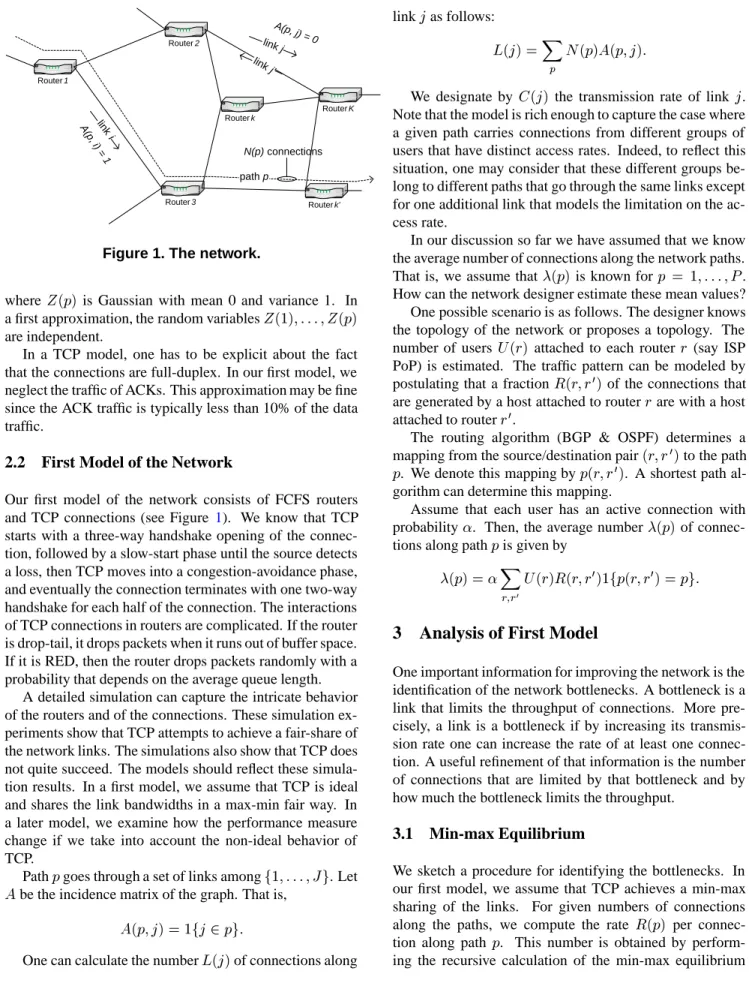
Router 1 Router 3 Router K Router 2 Router k Router k' link j link j' path p N(p) connections link i A(p, i) = 1 A(p, j) = 0
Figure 1. The network.
whereZ(p) is Gaussian with mean 0 and variance 1. In
a first approximation, the random variablesZ(1);:::;Z(p)
are independent.
In a TCP model, one has to be explicit about the fact that the connections are full-duplex. In our first model, we neglect the traffic of ACKs. This approximation may be fine since the ACK traffic is typically less than 10% of the data traffic.
2.2
First Model of the Network
Our first model of the network consists of FCFS routers and TCP connections (see Figure 1). We know that TCP starts with a three-way handshake opening of the connec-tion, followed by a slow-start phase until the source detects a loss, then TCP moves into a congestion-avoidance phase, and eventually the connection terminates with one two-way handshake for each half of the connection. The interactions of TCP connections in routers are complicated. If the router is drop-tail, it drops packets when it runs out of buffer space. If it is RED, then the router drops packets randomly with a probability that depends on the average queue length.
A detailed simulation can capture the intricate behavior of the routers and of the connections. These simulation ex-periments show that TCP attempts to achieve a fair-share of the network links. The simulations also show that TCP does not quite succeed. The models should reflect these simula-tion results. In a first model, we assume that TCP is ideal and shares the link bandwidths in a max-min fair way. In a later model, we examine how the performance measure change if we take into account the non-ideal behavior of TCP.
Pathpgoes through a set of links amongf1;:::;Jg. Let Abe the incidence matrix of the graph. That is,
A(p;j)=1fj2pg:
One can calculate the numberL(j)of connections along
linkjas follows:
L(j)= X
p
N(p)A(p;j):
We designate by C(j)the transmission rate of link j.
Note that the model is rich enough to capture the case where a given path carries connections from different groups of users that have distinct access rates. Indeed, to reflect this situation, one may consider that these different groups be-long to different paths that go through the same links except for one additional link that models the limitation on the ac-cess rate.
In our discussion so far we have assumed that we know the average number of connections along the network paths. That is, we assume that(p)is known for p = 1;:::;P.
How can the network designer estimate these mean values? One possible scenario is as follows. The designer knows the topology of the network or proposes a topology. The number of users U(r) attached to each routerr (say ISP
PoP) is estimated. The traffic pattern can be modeled by postulating that a fractionR (r;r
0
)of the connections that
are generated by a host attached to routerrare with a host
attached to routerr 0
.
The routing algorithm (BGP & OSPF) determines a mapping from the source/destination pair(r;r
0
)to the path p. We denote this mapping byp(r;r
0
). A shortest path
al-gorithm can determine this mapping.
Assume that each user has an active connection with probability. Then, the average number(p)of
connec-tions along pathpis given by
(p)= X r;r 0 U(r)R (r;r 0 )1fp(r;r 0 )=pg:
3
Analysis of First Model
One important information for improving the network is the identification of the network bottlenecks. A bottleneck is a link that limits the throughput of connections. More pre-cisely, a link is a bottleneck if by increasing its transmis-sion rate one can increase the rate of at least one connec-tion. A useful refinement of that information is the number of connections that are limited by that bottleneck and by how much the bottleneck limits the throughput.
3.1
Min-max Equilibrium
We sketch a procedure for identifying the bottlenecks. In our first model, we assume that TCP achieves a min-max sharing of the links. For given numbers of connections along the paths, we compute the rate R (p) per
connec-tion along path p. This number is obtained by
9 10
6
2
4
p
1p
2p
3j
1j
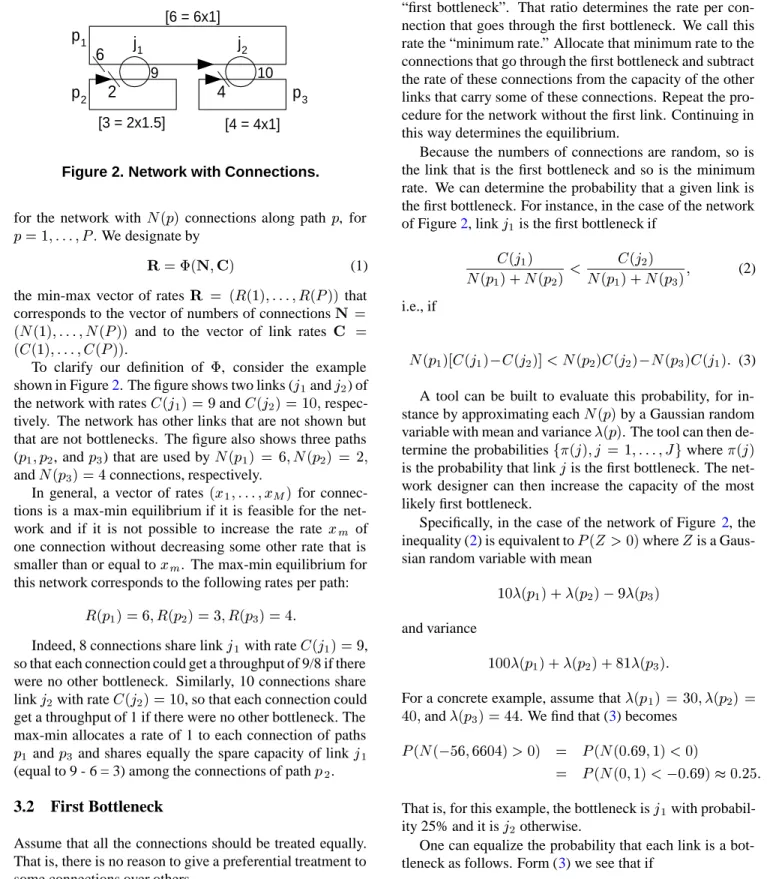
2 [6 = 6x1] [4 = 4x1] [3 = 2x1.5]Figure 2. Network with Connections.
for the network with N(p) connections along pathp, for p=1;:::;P. We designate by
R=(N;C) (1)
the min-max vector of ratesR = (R (1);:::;R (P))that
corresponds to the vector of numbers of connectionsN= (N(1);:::;N(P)) and to the vector of link rates C = (C(1);:::;C(P)).
To clarify our definition of , consider the example
shown in Figure2. The figure shows two links (j 1and
j 2) of
the network with ratesC(j 1
)=9andC(j 2
)=10;
respec-tively. The network has other links that are not shown but that are not bottlenecks. The figure also shows three paths (p
1 ;p
2, and p
3) that are used by N(p 1 ) =6;N(p 2 ) = 2; andN(p 3 )=4connections, respectively.
In general, a vector of rates (x 1
;:::;x M
)for
connec-tions is a max-min equilibrium if it is feasible for the net-work and if it is not possible to increase the rate x
m of
one connection without decreasing some other rate that is smaller than or equal tox
m. The max-min equilibrium for
this network corresponds to the following rates per path:
R (p 1 )=6;R (p 2 )=3;R (p 3 )=4:
Indeed, 8 connections share linkj
1with rate C(j
1 )=9,
so that each connection could get a throughput of 9/8 if there were no other bottleneck. Similarly, 10 connections share linkj
2with rate C(j
2
)=10, so that each connection could
get a throughput of 1 if there were no other bottleneck. The max-min allocates a rate of 1 to each connection of paths
p 1and
p
3 and shares equally the spare capacity of link j
1
(equal to 9 - 6 = 3) among the connections of pathp 2.
3.2
First Bottleneck
Assume that all the connections should be treated equally. That is, there is no reason to give a preferential treatment to some connections over others.
Note that the min-max equilibrium is easy to identify. First compute, for each link, the ratio of the link rate divided by the number of connections that go through it. The min-imum of these ratios is achieved by a link that we call the
“first bottleneck”. That ratio determines the rate per con-nection that goes through the first bottleneck. We call this rate the “minimum rate.” Allocate that minimum rate to the connections that go through the first bottleneck and subtract the rate of these connections from the capacity of the other links that carry some of these connections. Repeat the pro-cedure for the network without the first link. Continuing in this way determines the equilibrium.
Because the numbers of connections are random, so is the link that is the first bottleneck and so is the minimum rate. We can determine the probability that a given link is the first bottleneck. For instance, in the case of the network of Figure2, linkj
1is the first bottleneck if C(j 1 ) N(p 1 )+N(p 2 ) < C(j 2 ) N(p 1 )+N(p 3 ) ; (2) i.e., if N(p 1 )[C(j 1 ) C(j 2 )]<N(p 2 )C(j 2 ) N(p 3 )C(j 1 ): (3)
A tool can be built to evaluate this probability, for in-stance by approximating eachN(p)by a Gaussian random
variable with mean and variance(p). The tool can then
de-termine the probabilitiesf(j);j =1;:::;Jgwhere(j)
is the probability that linkjis the first bottleneck. The
net-work designer can then increase the capacity of the most likely first bottleneck.
Specifically, in the case of the network of Figure 2, the inequality (2) is equivalent toP(Z>0)whereZis a
Gaus-sian random variable with mean
10(p 1 )+(p 2 ) 9(p 3 ) and variance 100(p 1 )+(p 2 )+81(p 3 ):
For a concrete example, assume that(p 1 )=30;(p 2 )= 40;and(p 3
)=44. We find that (3) becomes P(N( 56;6604)>0) = P(N(0:69;1)<0)
= P(N(0;1)< 0:69)0:25:
That is, for this example, the bottleneck isj
1with
probabil-ity 25% and it isj
2otherwise.
One can equalize the probability that each link is a bot-tleneck as follows. Form (3) we see that if
(p 1 )[C(j 1 ) C(j 2 )]=(p 2 )C(j 2 ) (p 3 )C(j 3 );
then each link is a bottleneck with equal probabilities. How-ever, the case of a general network is more complex.
3.3
Rate per Connection
One useful measure of performance is the rate per TCP con-nection. A numerical tool can evaluate this rate as follows. Recall from (1) that the rate is some function of the numbers of connections. If we know the distribution of the number of connections, we can determine, in principle, the distribu-tion of the rate per connecdistribu-tion. We illustrate the calculadistribu-tions that the tool must perform for the network of Figure 2. To simplify the notation, let
x i = N(p i )andR i =R (p i );i=1;2;3; C k = C(j k );k=1;2:
With this notation, the identity (1) can be written as
R 1 = min f C 1 x 1 +x 2 ; C 2 x 1 +x 3 g R 2 = C 1 x 1 R 1 x 2 R 3 = C 2 x 1 R 1 x 3 :
A numerical integration tool can determine the probabil-ity that these rates are acceptably large. For instance, one design objective might be that these rates should all be at least equal to 0.1 (say 0.1Mbps) with a high probability. For our numerical example, we must evaluate the following probability: P(x 1 +x 2 90andx 1 +x 3 100): Sincex 1 +x 2and x 1 +x
3are associated random
vari-ables, this probability is larger than
P(x 1 +x 2 90)P(x 1 +x 3 100) =P(N(70;70)90)P(N(74;74)100) =P(N(0;1)2:4)P(N(0;1)3)0:99
which may be an acceptable design objective.
A numerical tool could perform the calculation without using the lower bound. One possible method for doing this calculation for a large network is by a Monte Carlo simu-lation. In such a simulation, one first generates a random vectorxof the numbers of connections along the different
paths. One then checks whether the inequalities are satis-fied. The number of random variables to generate is equal to the number of paths and the number of inequalities to verify is equal to the number of links. One can estimate the number of random vectors to generate as follows. For a given random vectorx
n, let f(x
n
)be equal to 0 if the
inequalities are satisfied and to 1 otherwise. We want to estimateEf(x n )by computing f(x 1 )++f(x n ) :
Standard arguments show that to be within a few percent of the correct value with probability 95% one has to generate approximately n = 200=Ef(x
n
) trials. ForEf(x n
) 1%, one has to generate approximately20;000trials. The
complexity of the simulation is linear in the product of the number of paths times the number of links.
4
Model Uncertainties
As we stated at the outset, to be useful a tool must be able to examine the effect of model uncertainties. In our prototype, we examine one source of uncertainty: the departure from fairness of TCP.
4.1
Note on TCP Bias
Simulations and analysis show that TCP is biased in fa-vor of connections with a shorter round-trip time. For in-stance, if persistent connections share a single bottleneck, then the throughput of a connection is roughly inversely proportional to its propagation time. The bias is reduced when the routers implement RED (random early drop) and also when the network implements ECN (explicit conges-tion notificaconges-tion). Nevertheless, the bias remains signifi-cant. Versions of TCP that almost eliminate this bias have been developed. One of these versions is TCP-Vegas. An-other method to reduce the bias is to use a form of per flow queuing in the routers. These mechanisms are rarely imple-mented.
The bias of TCP is more difficult to predict in a network with many bottlenecks. Simulations show that a reason-able estimate of the bias still corresponds to a throughput inversely proportional to the round-trip time.
The ratio of propagation times of connections that share a common router can be rather large. The maximum value of this ratio could be estimated by examining the network topology.
4.2
Analysis of Effect of TCP Bias
For the purpose of our study, we assume that the ratio of propagation times is bounded by 10. This range of prop-agation times translates into departures from the fair equi-librium. For instance, in the network of Figure 2, assume that the propagation time of pathp
1is ten times larger than
that of pathsp 2and
p
3. To study the effect of these
propa-gation times, first assume that linkj
1 is the bottleneck. In
that case, connections along pathp
1get a rate R
1that is ten
times smaller than the rateR
2of the connections along path p 2. Consequently, 9=6R 1 +2R 2 =6R 1 +20R 1 =26R 1 ;
so thatR 1
0:35. Second, assume that linkj
2 is the
bot-tleneck. The corresponding constraint becomes
10=6R 1 +4R 3 =6R 1 +40R 1 =46R 1 ; so thatR 1
0:22. We conclude that linkj
2is the
bottle-neck and the rates are
R 1 0:22;R 2 = 9 6R 1 2 3:8;R 3 = 10 6R 1 4 2:2:
More generally, this procedure can be applied to deter-mine the rates that correspond to a given maximum value of the ratio of propagation times. The tool can include these calculations and take them into account when computing the probability that all the connections get a specific mini-mum rate. We illustrate this calculation in the case of the network of Figure2where we assume that the numbers of connections are random as in Section3.2. We want to com-pute a rateso that the probability that the connections get
at least a rate equal to is at least 95%. By combining
the method of Section3.2and the ratio of 10 for the prop-agation times, we see that we must calculate the following probability: P( 9 x 1 +10x 2 and 10 x 1 +10x 3 ):
This probability is the same as the following one:
P(x 1 +10x 2 9=andx 1 +10x 3 10=):
A lower bound on this probability is
P(x 1 +10x 2 9 ))P(x 1 +10x 3 10 ) =P(N(430;4030) 9 )P(N(470;4430) 10 ) P(N(0;1)0:14 6:8)P(N(0;1)0:15 7) where = 1
. We find that =110guarantees that this
lower bound is at least 95%. Consequently, the guaranteed bandwidth per connection is=1=110=910
3
. Re-call that if TCP was not biased we could guarantee a rate
0:1to each connection. This simple example shows that it
is essential for the tool to be able to take such a bias into account.
5
Classes of Service
In this section, we explore how we can predict the effect of classes of service. We first explain what we mean by class of service. We then discuss an example of analysis.
5.1
CoS Implementation
When implementing class of service (CoS), a router clas-sifies packets based on the type of service field of the IP
1 q
w
1w
qC
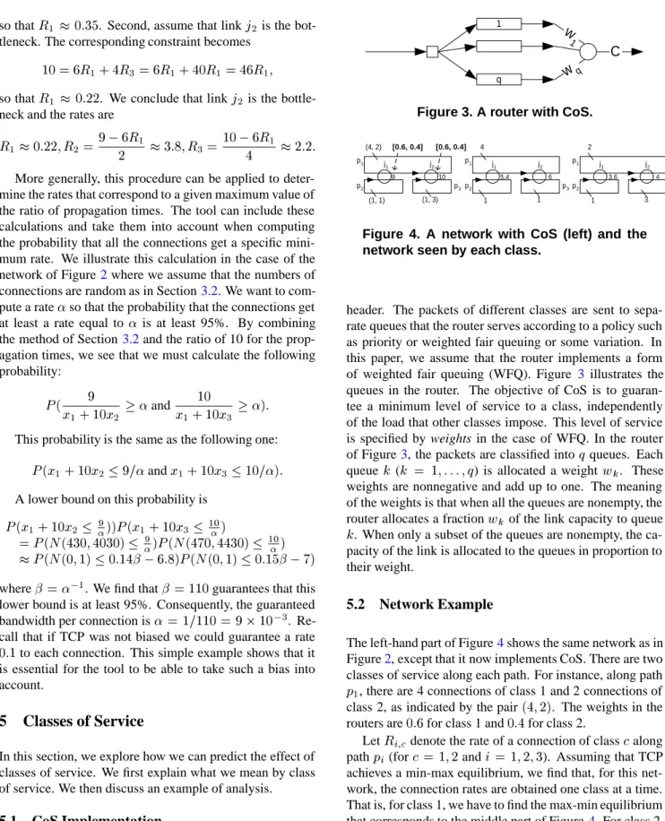
Figure 3. A router with CoS.
5.4 6 4 1 1 p1 p2 p3 j1 j2 3.6 4 2 1 3 p1 p2 p3 j1 j2 9 10 (4, 2) (1, 1) (1, 3) p1 p2 p3 j1 j2 [0.6, 0.4] [0.6, 0.4]
Figure 4. A network with CoS (left) and the network seen by each class.
header. The packets of different classes are sent to sepa-rate queues that the router serves according to a policy such as priority or weighted fair queuing or some variation. In this paper, we assume that the router implements a form of weighted fair queuing (WFQ). Figure 3 illustrates the queues in the router. The objective of CoS is to guaran-tee a minimum level of service to a class, independently of the load that other classes impose. This level of service is specified by weights in the case of WFQ. In the router of Figure3, the packets are classified intoqqueues. Each
queuek (k = 1;:::;q) is allocated a weightw
k. These
weights are nonnegative and add up to one. The meaning of the weights is that when all the queues are nonempty, the router allocates a fractionw
k of the link capacity to queue k. When only a subset of the queues are nonempty, the
ca-pacity of the link is allocated to the queues in proportion to their weight.
5.2
Network Example
The left-hand part of Figure4shows the same network as in Figure2, except that it now implements CoS. There are two classes of service along each path. For instance, along path
p
1, there are 4 connections of class 1 and 2 connections of
class 2, as indicated by the pair(4;2). The weights in the
routers are0:6for class 1 and0:4for class 2.
LetR
i;cdenote the rate of a connection of class calong
pathp i(for
c =1;2andi =1;2;3). Assuming that TCP
achieves a min-max equilibrium, we find that, for this net-work, the connection rates are obtained one class at a time. That is, for class 1, we have to find the max-min equilibrium that corresponds to the middle part of Figure 4. For class 2, we have to find the max-min equilibrium for the network in the right-hand part of the figure.
we find the following rates: R 1;1 =1:08;R 2;1 =1:08;R 3;1 =1:68 R 1;2 =0:8;R 2;2 =2;R 3;2 =0:8:
Comparing these rates with those shown in Figure 2, we can see the effect of introducing the class of service in the network. You will note that this effect is not straightforward and that suitable tools are needed to quantify it.
Note that in general, the determination of the rates of the connections cannot be done simply one class at a time. For instance, if one class does not saturate the rate that the router guarantees to it, then the unused rate becomes available to the other classes. However, the algorithm to compute the rates is a simple extension of the method we have described. More generally, we see that the tool that we have de-scribed in the previous section can be used to evaluate the throughput of the different classes of service in a CoS net-work. The tool can also consider the bias of TCP and the randomness of the number of connections. This tool could be used to determine the suitable weights in the routers to achieve some target minimum rates for the different classes with a high probability. The analysis can be adapted easily to the case where the routers implement a priority schedul-ing combined with weighted fair queuschedul-ing.
6
Conclusions
We argued that useful network engineering tools must produce robust results, be able to include results from mea-surements and simulations, and be helpful for design.
To illustrate these requirements, we proposed a prototype tool for predicting the performance of TCP connections in a network with or without CoS. This prototype uses statistics on user activity to model the number of connections along network paths. The prototype uses simulation results about TCP to quantify its bias.
The features of the tool that we propose include the fol-lowing:
The rates of TCP connections are not specified a priori
by the sources. Rather, the rates are the result of the window-adjustment mechanism of TCP.
The number of connections that use the network is
ran-dom.
The tool takes into account departures from fairness of
TCP.
The effect of CoS can be quantified. The tool can be used for network design.
To convert this prototype into a tool that can be used for guiding the evaluation or the design of networks, the algo-rithms and numerical procedures need to be implemented.
Acknowledgments
This research was performed while the author was on leave with Odyssia Systems, Inc. Special thanks to Ra-jarshi Gupta, Matthew Siler, Linhai He, and Eric Chi for their comments.
7
References
[1] Floyd, S., and Jacobson, V., “Link-sharing and Resource Management Models for Packet Networks,” IEEE/ACM Transactions on Networking, Vol. 3 No. 4, pp. 365-386, August 1995.
[2] Ramakrishnan, K.K., and Floyd, S., “A Proposal to add Explicit Congestion Notification (ECN) to IP.” RFC 2481, January 1999.
[3] J. Mo, R. La, and J. Walrand, ”Analysis and Comparison of Reno and Vegas,” INFOCOM’99
[4] http://www-mash.cs.berkeley.edu/ns/
[5] Paxson, V., and Floyd, S., “Why We Don’t Know How To Simulate The Internet,” Proceedings of the 1997 Winter Simulation Conference, December 1997.