econ
stor
Der Open-Access-Publikationsserver der ZBW – Leibniz-Informationszentrum Wirtschaft The Open Access Publication Server of the ZBW – Leibniz Information Centre for Economics
Nutzungsbedingungen:
Die ZBW räumt Ihnen als Nutzerin/Nutzer das unentgeltliche, räumlich unbeschränkte und zeitlich auf die Dauer des Schutzrechts beschränkte einfache Recht ein, das ausgewählte Werk im Rahmen der unter
→ http://www.econstor.eu/dspace/Nutzungsbedingungen nachzulesenden vollständigen Nutzungsbedingungen zu vervielfältigen, mit denen die Nutzerin/der Nutzer sich durch die erste Nutzung einverstanden erklärt.
Terms of use:
The ZBW grants you, the user, the non-exclusive right to use the selected work free of charge, territorially unrestricted and within the time limit of the term of the property rights according to the terms specified at
→ http://www.econstor.eu/dspace/Nutzungsbedingungen By the first use of the selected work the user agrees and declares to comply with these terms of use.
zbw
Leibniz-Informationszentrum WirtschaftGundlach, Erich
Article
Regional convergence of output
per worker in China : a neoclassical
interpretation
Asian economic journal
Provided in cooperation with: Institut für Weltwirtschaft (IfW)
Suggested citation: Gundlach, Erich (1997) : Regional convergence of output per worker in China : a neoclassical interpretation, Asian economic journal, ISSN 1351-3958, Vol. 11, Iss. 4, pp. 423-442, doi:10.1111/1467-8381.00046 , http://hdl.handle.net/10419/1765
Regional Convergence of Output per Worker in China:
A Neoclassical Interpretation
by
Erich Gundlach
Kiel Institute of World Economics August 1997
Regional Convergence of Output per Worker in China:
A Neoclassical Interpretation
Abstract
Regional output per worker has converged across Chinese provinces in 1979-1989. The estimated rate of convergence is 2.2 percent. This rate of convergence can be explained by neoclassical growth model conditional on assumptions about factor mobility and production elasticities. My empirical results show that capital mobility has been high across Chinese provinces and that the production elasticity of human capital is about twice as high as the production elasticity of physical capital. With less interprovincial capital flows as the result of an expected increase in fiscal decentralization, the rate of convergence of regional output per worker is likely to decline.
Chinese provinces display large differences in growth rates and output per worker. Growth rates have differed by a factor of eight, and output per worker has differed by a factor of nine. However, these large differences have tended to decline over time, because poor provinces have grown faster than rich provinces since the beginning of economic reform in 1978. Figure 1 highlights this stylized fact as a negative correlation between output per worker in 1978 and average annual growth rates in 1978-1989.1 That is, regional output per worker has converged across Chinese provinces in 1978-1989.2
The traditional neoclassical model of economic growth (Solow 1956, Mankiw et al. 1992) explains convergence of output per worker as an adjustment to a steady state, which is determined by the rate of factor accumulation. This model implies that the rate of convergence depends on specific parameters such as production elasticities, depreciation rates, and labor force growth. Because these parameters can be estimated, the neoclassical model can be used to derive a quantitative prediction for the rate of convergence that, in turn, can be compared
* This paper reports research undertaken in a project on "Decentralization and Enterprise Reform in China". I thank two anonymous referees and Martin Raiser for helpful comments on an earlier version. Financial support by the Volkswagen-Stiftung is gratefully acknowledged.
1 The Appendix gives a definition of variables and the respective data sources. Two Appendix tables contain all the data used in this paper. The data refer to 29 Chinese provincial level localities, including 22 provinces, 3 municipalities under the central government, and 4 autonomous regions (Tibet is excluded due to data limitations). I refer to all these entities as provinces.
2 Figure 1 actually reflects convergence and not Galton's fallacy (see Friedman (1992)) because the coefficient of variation of output per worker declines from 0.70 in 1978 to 0.51 in 1989.
with the observed rate of convergence. Thus, the neoclassical model of economic growth may provide a reasonable account of the convergence of output per worker across Chinese provinces if the theoretically predicted rate of convergence closely matches the observed rate of convergence.
One serious objection can be raised against the use of the neoclassical growth model for an explanation of convergence in the case of China. China is a socialist economy where the basic principles underlying the neoclassical growth model may not apply, namely the maximization of life time consumption by consumers and the maximization of profits by firms. However, one could imagine a benevolent social planner who seeks to maximize the utility of the representative family. Despite its lack of realism, from a purely theoretical point of view such an assumption guarantees that the central planning solution of the model will be the same as that for the decentralized economy if the planner has the same form of preferences as those assumed before (Barro and Sala-i-Martin 1995). Therefore, the application of the neoclassical growth model in the case of China is not as far fetched as it may appear at first sight.3
My empirical results show that the observed rate of convergence across Chinese provinces is rather slow, namely 2.2 percent. The neoclassical model can explain this rate of convergence if there is no capital mobility across Chinese provinces and if the production elasticity of capital is about 0.75. But I find that capital mobility appears to be high, because saving and investment
3 Another objection is that China is a developing country where the neoclassical assumption of full employment may be misleading. This objection is more difficult to reject as long as one cannot clarify whether China actually suffers from an unemployment equilibrium. For the neoclassical model to be applicable, it is sufficient to assume that there are forces which tend to equalize marginal factor products with real factor earnings. Such forces could be initiated by a market process, or, in the case of China, by a benevolent social planner trying to maximize welfare.
rates are uncorrelated across Chinese provinces. If one, therefore, assumes that Chinese provinces are open economies, the neoclassical model predicts that capital should move quickly to equalize marginal products and, hence, that convergence of output per worker will be rapid.
I can reconcile the observed and the theoretically predicted rate of convergence by introducing human capital as a third factor of production, and by assuming that human capital is immobile. If so, interprovincial borrowing would be possible to finance accumulation of physical capital, but not accumulation of human capital. With the human capital augmented neoclassical model, I find that the production elasticity of human capital is about twice as high as the production elasticity of physical capital, and that the combined production elasticity of all capital is about 0.8.
These findings imply that convergence of output per worker across Chinese provinces has been supported by high interprovincial physical capital mobility since the beginning of economic reforms in 1978. Capital mobility has allowed poor regions to maintain a high rate of physical capital accumulation despite low saving rates. But interprovincial capital mobility is likely to decline once fiscal decentralization gains further momentum in the course of Chinese economic reforms, at least as long as an efficient domestic capital market is largely missing. As a result, regional convergence of output per worker would be likely to decline as well.
2. The Rate of Convergence: Theory and Evidence
Suppose that all Chinese provinces have access to the same technology and Chinese workers across provinces share the same set of preferences, which have the same form as those of the benevolent social planner. Then, the traditional neoclassical growth model (Solow 1956) predicts convergence of output per
worker to a common steady state. Following Barro and Sala-i-Martin (1992), convergence to the steady state between times 0 and T can be described by
(1)
(
)
(
)
(
)
1 1 0 0 T Y L Y L B e T Y L T i i T i log / / log / ⎡ ⎣ ⎢ ⎤ ⎦ ⎥ = −⎛⎝⎜ − ⎞⎠⎟ −λ ,where
(
Y / L)
i is output per worker in province i, Bis a constant term, and λ is the convergence rate. That is, the growth rate of output per worker is a negative function of initial output per worker.A regression of the average annual growth rate of output per worker in 1978-1989 on output per worker in 1978 across the 29 Chinese provinces shown in Figure 1 delivers the following result (standard errors in parenthesis):
(2) ln
(
Y / L)
1989 −ln(
Y / L)
1978 = 1 93. − 0 22. ln(
Y / L)
1978 (0.43) (0.06) No. of observations = 29. R2 = 0.28 s e e. . . = 0.17 Implied λ = 0 022 0 007 . ( . ) .The point estimate of the convergence rate of 2.2 percent lies within the range that is known from other empirical studies of convergence.4 A λ of about
2 percent implies that convergence towards the steady state will proceed rather slowly, because in this case half of the departure from a given steady state would remain for 35 years. Two questions arise. First, whether any theoretical parameterization of the neoclassical model would actually produce a
convergence rate in the range of 2 percent and, second, whether such a parameterization is indeed supported empirically for the case of China..
The theoretical convergence rate can be derived as follows. The neoclassical model takes the rates of saving, population growth and technological progress as exogenous. Output (Y) is produced under constant returns to scale with two inputs, capital (K) and labor (L), which are paid their marginal products. Assuming a Cobb-Douglas production function, output at time t is given by: (3) Yt =Ktα
(
A Lt t)
1−α , 0<α<1 .A, the level of technology, and L are assumed to grow exogenously at rates g
and n, so At = A e0 gt and Lt = L e0 nt. Hence, the number of effective units of labor, A Lt t, grows at rate g +n. Furthermore, assuming constant saving (S Y/ ) and depreciation rates (δ = D K/ ), and defining k as the stock of capital per effective unit of labor (k =K / AL) and y as output per effective unit of labor (y=Y AL/ ), it can be shown that the evolution of k is governed by (Mankiw et al. 1992) 5
(4) dk dt/ = sy− + +
(
n g δ)
k ,and that k converges to a steady state value (5) k*=
[
s/(
n+ +g δ)
]
1 1/( −α) .Taking the first order Taylor expansion of the right hand side of equation (4) and substituting for s using the steady state condition (5) gives (Mankiw 1995)
(6) dk dt/ = −λ
(
k −k*)
,where the rate of convergence to the steady state is given by
(7) λ = −
(
1 α)
(
n+ +g δ)
,with α as the production elasticity of capital (see equation 3). If λ is known to be about 2 percent, equation (7) can be used to infer an estimate for α, conditional on (n+ +g δ ).
The standard parameterization suggested in the literature is (n+ + =g δ 0 08. ), with a rate of labor force growth of 1 percent, a rate of technological change of 2 percent, and a depreciation rate of 5 percent (Barro et al. 1995). Because the observed rate of convergence is about 2 percent, equation (7) then would imply that α is about 0.75.
An implied value of α of about 0.75 creates a first problem for the traditional neoclassical growth model. According to the assumptions of perfect competition, which is equal to the assumption of optimal planning in the case of a benevolent social planner, and constant returns to scale, α should equal capital's share in income. The average value for α calculated from the national accounts of industrialized countries is about 0.3 (Maddison 1987). But the national accounts do not account for human capital formation. Therefore, a higher value of α can be justified as a production elasticity for a broad concept of capital that includes physical and human capital (Barro and Sala-i-Martin 1992; Mankiw et al. 1992). Hence, the traditional neoclassical model should be augmented by human capital as a third factor of production.
A second, more serious problem for the traditional neoclassical growth model arises from the implicit assumption of capital immobility. While this assumption may be a reasonable approximation for cross-country studies, it is rather unlikely to hold within countries. Whether regional capital mobility holds for socialist economies like China is an empirical question (see below). But with regional capital mobility, the theoretically predicted rate of convergence towards
the steady state would be high, because capital would move quickly to equalize marginal products.
The theoretical solution for both problems is an open-economy version of the neoclassical growth model (Barro et al. 1995) that assumes interregional mobility of physical capital flows, but immobile human capital. The human capital augmented production function reads
(8) Y =K Hα β
( )
AL 1− −α β 0<α β+ <1 ,where A grows at rate g and L grows at rate n as before, and H is the level of human capital. Calculating the steady state values k* and h* (h=H / AL) similar to equation (5) and substituting them into the production function (8) gives the reduced form as
(9) lnY / L= −c + ln
(
n g)
− − + + α β α β δ 1 + − −(
)
α α β 1 ln ΔK Y/(
)
+ − − β α β 1 ln ΔH Y/ ,where c equals lnA+gt, and (ΔK Y/ ) and (ΔH Y/ ) represent the investment rates for physical and human capital, which appear as right-hand-side variables instead of the respective saving rates in the open economy version of the model. Alternatively, combining the steady state equation for h* with equation (9) yields (10) ln /Y L= −c ln
(
n g)
− + + α α δ 1 + −(
)
α α 1 ln ΔK Y/ + −( )
β α 1 ln h* ,where it is the level of human capital per worker which enters as a right-hand-side variable, and not the investment rate of human capital as in equation (9).
For the open economy model, the rate of convergence to the steady state is given by (Barro et al. 1995)
(11) λ β
(
)
α δ
open =⎛⎝⎜1− − ⎞⎠⎟ n+ +g
1 .
To prove that equation (11) correctly predicts the observed rate of convergence, the empirical analysis has two tasks. First, it has to be shown that the assumption of physical capital mobility across Chinese provinces is reasonable. Second, it has to be shown that conditional on (n+ +g δ ), estimated production elasticities for physical and human capital can be used to predict a rate of convergence of 2.2 percent.
3. Estimating the Open Economy Model
3.1 Capital Mobility across Chinese Provinces
In China, as in all socialist economies, the fiscal system has traditionally played an overarching role in the allocation of investment. In the context of the neoclassical growth model, a benevolent social planner could decide on regional investment and regional saving in order to produce a welfare maximizing convergence of regional output per worker. But China has begun to decentralize its fiscal system and allows provincial governments to retain an increasing share of the revenue from local economic activity (Raiser 1996). This opens up the possibility that the interregional redistribution of capital flows through the fiscal system has been reduced. However, fiscal reform in China does not yield a clear pattern of decentralization (Zhang and Zou 1996): Budgeting spending became more decentralized, but extra-budgeting spending showed an increasing central share since 1978; the consolidated central spending share fluctuated and the central revenue share increased in 1982-1992. Thus, a benevolent social planner would have had the possibility to allocate investment across Chinese province.
Unfortunately, recent assessments of capital flows within China do not clearly show whether they have happened at all and if so, in which direction. The World Bank (1994) maintains that there is no evidence to support a convergence of
returns to capital across different provinces, suggesting that capital mobility is low at best. Raiser (1995) surveys the literature on fiscal decentralization which claims that capital mobility across Chinese provinces has declined. Nevertheless, Hsueh Tien-tung (1994) reports that during the 1980s the inflow of interregional capital to low income provinces has been as high as 25 percent or above of their national income, pointing to a rather high interprovincial capital mobility.
As a first attempt to get a clearer picture, I reproduce data on the fiscal balance of Chinese provinces. The underlying data have been calculated by Ma (1995a) for 1983 and 1991 and converted to the "percent of GDP" format by Raiser (1996). I focus on the data for 1983 which represent a midyear in my period of observations spanning 1978 to 1989 (see Table A1). A negative value of the fiscal balance indicates that the province has been a net receiver of fiscal transfers from the center.
The idea of a benevolent social planner who allocates investment across Chinese regions implies that there is a systematic relation between the flow of fiscal resources and the productivity (output per worker) of provinces. As it turns out, the correlation coefficients between my measure of fiscal balance in 1983 and output per worker, either in 1978 or in 1989, are positive and statistically significant. For provincial output per worker in 1978, I find a correlation coefficient of 0.65 with the fiscal balance in 1983; for output per worker in 1989, the correlation coefficient is 0.62.6
These findings demonstrate that fiscal resources have tended to flow from high productivity to low productivity provinces in China in 1978-1989. Since the observed correlation is not perfect, this is not to deny that other motives than
6 The correlation coefficient between output per worker in 1989 and fiscal balance in 1991 (not shown in Table A1) is somewhat lower, namely 0.52. This lower correlation may indicate the increasing fiscal decentralization in recent years.
regional convergence have also played a role for the redistribution of fiscal funds. E.g., a negative fiscal balance may primarily reflect the financing by the center of the exploitation of mineral resources or strategic considerations rather than an attempt to achieve convergence of regional productivity and, thereby, per capita incomes. Nevertheless, the statistically significant positive correlation between fiscal balance and output per worker reveals that there is at least some empirical support for the assumed allocation mechanism by which capital should move from rich to poor provinces. The remaining question is whether the present result can be interpreted as capital mobility in the sense of the neoclassical model.
I use the approach suggested by Feldstein and Horioka (1980) to check whether the previous positive correlation between fiscal balance and output per worker can be interpreted as a form of capital mobility. If Chinese provinces are closed economies, their saving rates must equal their investment rates. But if they are open, their saving and investment rates could differ due to interprovincial capital movements through the fiscal system. Hence, the degree of capital mobility can be estimated by a regression of the investment rate (I Y/ ) on the saving rate (S Y/ ) across Chinese provinces:
(12)
(
I Y/)
it = +c γ(
S Y/)
ti ,where γ is the so-called savings retention coefficient. If γ equals 1, any change in the saving rate in province i leads to an identical change in the investment rate of province i. Thus, a γ of 1 would imply that province i is a closed economy, because no net interprovincial capital flows occur. By contrast, if γ
equals 0, investment and saving rates are uncorrelated at the provincial level. In this case, perfect interprovincial capital mobility would prevail.7
I use average saving and investment rates for various time periods to estimate the saving retention coefficient γ according to equation (12).8 This procedure is
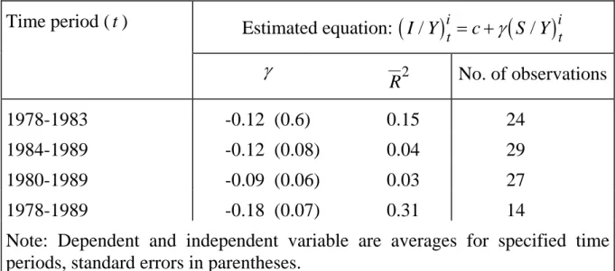
likely to bias upward the estimate for γ (Sinn 1992), i.e., towards finding capital immobility. However, the results in Table 1 show that saving and investment rates across Chinese provinces are uncorrelated since the savings retention coefficient is statistically not different from zero in three out of four cases.
The only statistically significant savings retention coefficient arises for average saving and investment rates in 1978-1989. However, the estimated coefficient is negative and, therefore, is also compatible with the view that during the 1980s, the central planning authorities still held a certain power of control over the regional distribution of capital accumulation (Hsueh Tien-tung 1994). Taken at face value, the negative saving retention coefficient implies that any increase in the average provincial saving rate would reduce that province's investment rate. But since this finding is based on 14 observations only, it may
7 Many authors have criticized the Feldstein-Horioka approach by showing that a high saving retention coefficient, especially in a time series context, does not necessarily imply the absence of capital mobility. By contrast, the interpretation of a statistically insignificant saving retention coefficient as an indicator of capital mobility is not disputed in the literature. E.g., Montiel (1994) uses the Feldstein-Horioka approach in this way and finds a surprisingly high degree of capital mobility for many DCs. For a brief survey of the empirical evidence on the relation between saving and investment rates from cross-country and inter-regional studies and for the controversies with regard to an interpretation of the saving retention coefficient that have arisen in the literature, see Feldstein (1994).
reflect the statistical properties of a special sample and should, therefore, not be overinterpreted. The results for the other samples confirm the view that capital has been mobile across Chinese provinces.
Taken together, I interpret my findings as indicating high capital mobility across Chinese provinces. High capital mobility would be compatible with a low rate of convergence under two scenarios, one empirical and one theoretical. First, the economic efficiency of interprovincial capital flows may be low, as suggested by Hsueh Tien-tung (1994), or, second, human capital may be less mobile than physical capital, as assumed by the neoclassical growth model for the open economy.
If the efficiency of interprovincial capital flows is low, the assumption of a welfare maximizing benevolent social planner could not be maintained for a consistent interpretation of the empirical facts. But without this assumption, it is difficult to explain how China, as a socialist economy, has managed to achieve average annual growth rates of real GDP per capita of about 8 percent during the 1980s (World Bank 1995). Therefore, it may be more useful to employ the augmented Solow model for the open economy for an explanation of the observed rate of convergence. The empirical relevance of this approach can be assessed by estimating production elasticities for physical and human capital according to equations (9) and (10). If α and β are known, it is possible to predict λ according to equation (11). This prediction can be compared with the estimated value for λ of 2.2 percent.
3.2 Production Elasticities for Physical and Human Capital
The main problem with estimating production elasticities according to equations (9) and (10) is that in contrast to flow measures of physical capital formation such as the investment rate (I Y/ ), direct flow or stock measures of human capital formation are generally not available. For a start, I use two alternative
indirect measures of human capital formation. The number of students enrolled in secondary education divided by the population (SCHOOL) is my flow measure, i.e., this variable is expected to proxy investment in human capital. The number of newspapers, magazines, and books published divided by the labor force (PUBL) is my stock measure, i.e., this variable is expected to proxy the
accumulated investment in human capital. As is self-evident, both proxies are
rather crude measures of human capital formation and, therefore, deserve second thoughts.
Schooling rates (SCHOOL) as a measure of investment in human capital have been used in recent international cross section studies of the empirics of growth.9 The general idea behind this measure is that variations in the fraction of the population devoted to formal education reflect variations in investment in human capital. The plausibility of this concept largely depends on the existence of different educational systems with different levels of education across the units of observation. Thus, this concept is more likely to produce reasonable results when applied across countries rather than when applied within countries. This is all the more so in the case of a centrally planned economy such as China. These considerations raise some doubts on the usefulness of SCHOOL as a measure of investment in human capital in the context of Chinese provinces. Nevertheless, SCHOOL is used in the following empirical analysis because no other proxies for investment in human capital can be derived from the provincial statistics in Hsueh et al. (1993).
Publications per worker (PUBL) as a measure of the stock of human capital seems to be even more dubious, at least at first sight. But this is not necessarily so. The assumption underlying this concept is that the provincial supply of
written information is correlated with the provincial quantity of human capital. Since the amount of written information is likely to be dominated by newspapers, PUBL will more or less reflect the consumption of newspapers per worker at the provincial level. Therefore, this measure may reflect factional differences in literacy rates across Chinese provinces which, in turn, may be more plausible measures of exogenous interprovincial differences in human capital than the reported schooling rates. This is not to deny that PUBL may vastly exaggerate the stock of human capital for a given year if publishing grew substantially following China's economic reforms. But what matters for the estimation of production elasticities is the structure of PUBL across provinces, which a priori is unlikely to be biased due to reform efforts.
Another problem with estimating production elasticities is the statistical precision required to be able to draw statistically significant inferences. This is all the more so if the production elasticities for physical and human capital turn out to be similar to those found for industrialized countries. In this case, the predicted convergence rates for the closed and the open economy versions of the neoclassical growth model may not differ by much (see Barro et al. 1995), and may become indistinguishable for production elasticities estimated with large standard errors.
One way to increase the statistical precision of the estimates is to restrict the regression equations (9) and (10). The restriction that can be imposed on equation (9) is that the regression coefficients on ln
(
n+ +g δ)
, ln(
ΔK Y/)
, and(
)
ln ΔH Y/ sum to zero. The restriction that can be imposed on equation (10) is that the regression coefficients on ln
(
n+ +g δ)
and ln(
ΔK Y/)
sum to zero. Taking into account these empirical modifications, the restricted empirical versions of equations (9) and (10) read(9a) ln
(
Y / L)
= +c[
ln(
I Y/)
ln(
n g)
]
− − − + +
α
α β δ
(
)
(
)
[
]
+ − − − + + β α β δ 1 ln SCHOOL ln n g and (10a) ln(
Y / L)
= +c[
ln(
I Y/)
ln(
n g)
]
− − + + α α δ 1 + −(
)
β α 1 ln PUBL . Table 2 presents the results of an OLS estimation of these specifications.10 Thespecification with the stock measure of human capital (10a) performs better with regard to statistical criteria such as R2 and p-value than the specification with the flow measure (9a). The p-value indicates that the restriction imposed on equation (9a) is rejected by the data at the 5 percent level of statistical significance, while the restriction imposed on equation (10a) is not rejected. The point estimates for α are not statistically different from each other and their size suggests that capital's share in income in China is not that different from capital's share in income in industrialized countries.11 However, the point
estimates for β differ. If investment in human capital (SCHOOL) is used as a right-hand-side variable, β is estimated to be about 0.16. But if the stock of human capital (PUBL) is used as a right-hand-side variable, β is estimated to be 0.46.
Several reasons exist why the point estimates for β may differ. First, the different estimates may simply reflect that the share of secondary education in income as measured by the production elasticity of SCHOOL is much smaller than the share of all human capital in income as measured by the production
10 The results presented in Table 2 are conditional on the previous assumptions that g equals 2 percent and δ equals 5 percent. The rate of labor force growth, n, can be directly observed for each Chinese province (see Table A1).
elasticity of PUBL. In this case, the more comprehensive measure is more likely to reflect the true impact of human capital formation on output per worker.
Second, the low estimate for β derived from the flow specification of human capital may be correct, while the high estimate for β derived from the stock specification of human capital may be biased upward due to a correlation between ln
(
PUBL)
and the disturbance term. Such a correlation could arise because changes in h, like changes in k, could depend on y. That is, if the accumulation of human capital is correctly described by the same data generating process as the accumulation of physical capital (see equation (4)), then ln(
PUBL)
will be correlated with the disturbance term in equation (10a). In this case, an OLS estimate of equation (10a) will produce an upward biased estimate of β.Third, PUBLcould be measured with error. This could happen if PUBL is an imperfect measure of the true variable, as indicated above. In this case, the true impact of human capital formation would even be larger than measured by the previous OLS estimate of β of about 0.46.12
Fourth, along the same lines, the low estimate for β derived from the investment specification of human capital could also result from a measurement error in SCHOOL. A measurement error would tend to bias downward the
12 Define the regression coefficients in equation (10a) as a=α / 1( −α) and
( )
b=β/ 1−α . It follows that β =b
(
1−(
1/(1+a))
)
. Thus, a downward biased estimate of b due to measurement error in PUBL would reduce the point estimate of β.implied point estimate for β.13 In this case, the true impact of human capital
formation would again be measured by the high estimate for β derived from the stock specification of human capital.14
I use Hausman's specification error test15 to reveal which of these possibilities
prevails, i.e., whether or not the covariance between my measures of human capital formation and the respective disturbances are zero. The Hausman test compares the parameters of the human capital measures derived under two alternative estimation techniques, standardized by the difference of the covariances of the two estimates. The first estimation by OLS assumes that the chosen specification is correct and, therefore, produces consistent results. The second estimation by Instrumental Variables (IV) could produce consistent results even if the chosen specification is incorrect and, therefore, would produce inconsistent results under OLS estimation. The test statistic to be derived under these assumptions is asymptotically Chi-squared, with a critical value of 6.63 (3.84) for the 1 (5) percent level of statistical significance for 1 degree of freedom.
13 Define the regression coefficients in equation (9a) as a=α / 1
(
− −α β)
and(
)
b=β/ 1− −α β . It follows that β =b/ 1( + +a b). Thus, a downward biased estimate of b due to measurement error in SCHOOL would reduce the point estimate of β. 14 A further reason for biased regression coefficients could arise from the potential
correlation between the variable measured with error and other variables in the equation. However, this problem does neither arise in equation (9a) nor in equation (10a), because both measures of human capital formation are uncorrelated with the measure of physical capital formation: The coefficient of correlation between ln
(
I Y/)
−ln(
n+ +g δ)
and(
)
ln SCHOOL −ln
(
n+ +g δ)
is 0.28 with an F-statistic of 2.39; the coefficient of correlation between ln(
I Y/)
−ln(
n+ +g δ)
and ln(
PUBL)
is 0.15 with an F-statistic of 0.65.I use PUBL as an instrument for SCHOOL and vice versa to see whether either SCHOOL or PUBL is independent from the disturbances in the unconstrained versions of equations (9a) and (10a) (see equations 9 and 10). Applying the Hausman test to the unconstrained version of equation (9a), I get a value of the test statistic of 22.55. This finding suggests that SCHOOL is correlated with the error term. Hence, the previous OLS parameter estimate on
SCHOOL seems to be biased (see Table 2). However, for the unconstrained
version of equation (10a), I get a value of the test statistic of 3.46. Therefore, the hypothesis that PUBL is uncorrelated with the error term cannot be rejected at the 5 percent level of statistical significance.
The results of the specification tests support the previous considerations regarding the appropriateness of PUBL and the inappropriateness of SCHOOL
as measures of human capital formation in the case of China. That is, based on comparisons of the OLS results in Table 2, the parameter estimate on PUBL
does not seem to be biased, at least not to the same degree as the parameter on
SCHOOL. By contrast, the parameter estimate on SCHOOL seems to be
downward biased due to measurement error. This leaves open the question how large the bias actually is.
I use an error in variables model to estimate the extent of the downward bias in the parameter estimate on SCHOOL. The classical errors in variables model amounts to running a reverse regression if one of two explanatory variables is measured with error.16 Hence, the variable presumed to be measured with error in equation (9a), ln
(
SCHOOL)
−ln(
n+ +g δ)
, enters as the dependent variable, and ln(
Y L/)
enters as a right-hand-side variable. As before, the resulting regression coefficients can be used to recover point estimates for α and β. Ifind a statistically significant point estimate of β of 0.74 (Table 3), which can be interpreted as an upper bound for β. The point estimate for α is inconsistent, but the standard error is large. This result confirms that the previous low estimate for β, which can be interpreted as a lower bound, is downward biased due to measurement error in my proxy for investment in human capital. As it turns out, the average of the lower an upper bound estimates of β from equation (9a) equals the OLS estimate of β from equation (10a), which can be considered as unbiased according to the results of the Hausman specification test.
Notwithstanding the results of the Hausman specification test at the 5 percent level of statistical significance, PUBL can only be considered as a rather crude proxy of the stock of human capital. To check for the possibility of a potential measurement error in PUBL, I also use the errors in variables model with
(
)
ln PUBL as the dependent variable. I find statistically significant point estimates for α of 0.23 and for β of 0.64 (Table 3). These findings largely confirm the results derived from the OLS estimation of equation (10a) (see Table 2, second column) with the new point estimate for β again interpreted as an upper bound. This new estimate is statistically indifferent from the lower bound OLS point estimate for β of 0.46.
Taken together, I interpret my findings as confirming the hypothesis that a high estimate of β in the range of 0.46 to 0.64 rather than a low estimate in the range of 0.16 is more likely to measure the true impact of human capital formation on output per worker in China. The implication of this finding is that the impact of human capital formation is about twice as large as the impact of
physical capital accumulation, since α is estimated to be about 0.25.17 Hence, a
production function that is compatible with my regression results reads
Y =K0 25. H0.55L0 20. . The remaining question is whether the estimated production elasticities predict a rate of convergence that closely matches the observed rate of convergence of about 2 percent.
3.3 The Predicted Rate of Convergence
Once the two production elasticities α and β are known, equation (11) describes how the predicted rate of convergence can be derived for the case of the open economy, conditional on the rate of labor force growth (n), the rate of technological change (g), and the depreciation rate (δ). Of the three conditioning parameters, n is the only parameter that can be measured directly. I measure n as the average annual provincial growth rate of the labor force in 1978-1989, weighted by the labor force in 1989. I find that for my sample, the average growth rate of the labor force is 3 percent, so n = 0.03.
The rate of technological change can only be measured indirectly as a residuum, namely as the rate of total factor productivity growth. The problem with this procedure is that measured rates of technological change depend on the specification of the production function. Jefferson et al. (1992) estimate a production function with capital, labor, and intermediate inputs and find a rate of technological change of about 2 percent for Chinese state owned industry and of about 4 percent for Chinese collective industry. These results may serve as a first approximation of g, although human capital accumulation is not taken into account and the focus is on technological change in industry rather than in the aggregate economy. Another approximation may be derived from the estimates
for countries such as Taiwan and South Korea, which experienced similar growth rates as China in the 1980s. Taking into account human capital accumulation and focusing on the aggregate economy, Young (1995) finds average rates of total factor productivity growth of 1.6 percent for South Korea and of 2.4 percent for Taiwan. These results suggest that the standard parameterization of g of 2 percent may also be reasonable for the case of China. That is, I assume that g = 0.02, which is compatible with the findings for Chinese industry given that aggregate total factor productivity growth figures are usually somewhat lower than industry figures.
Reliable data on the stock of physical capital and its depreciation are not available for China, so the depreciation rate cannot be measured directly as well. Given that the share of depreciation in GDP is about 10 percent, which is an average figure for industrialized countries (Maddison 1987), the rate of depreciation can be calculated once the capital output ratio is known according to δ =
(
D Y/) (
/ K Y/)
. For leading industrial countries such as the United States, the capital output ratio is about 3, so δ would be about 3 percent (Mankiw et al. 1992). But for developing countries, it is reasonable to assume a smaller capital output ratio. For example, δ is 5 percent for a capital output ratio of 2. Actually, the capital output ratio may be even lower than 2 in developing countries, but then the share of depreciation in GDP may also be lower than 10 percent. On balance, therefore, I assume a depreciation rate of 5 percent for China, so δ = 0.05.With these parameterizations for (n+ +g δ ), the rate of convergence to the steady state can be calculated according to equation (11) as
(11a) λopen = − −
(
)
⎛ ⎝⎜ ⎞⎠⎟ + + = 1 0 55 1 0 25 0 03 0 002 0 05 0 027 . . . . . . .Hence in the case of China, the human capital augmented Solow model for the open economy predicts a rate of convergence of output per worker of 2.7 percent, which is somewhat higher than the actually observed rate of convergence of 2.2 percent. However, the difference between the two rates of convergence is not statistically significant. What is more, the estimated rate of convergence is also not statistically different from the rate of convergence predicted for the closed economy, which follows from
(7a) λclosed = −
(
(
+)
)
(
+ +)
= −(
−)(
+ +)
= 1 1 0 25 0 55 0 03 0 02 0 05 0 02 α β n g δ . . . . . . . That is, my empirical results are compatible with both the open and the closed economy version of the neoclassical growth model. One reason for this outcome may be that capital is not perfectly mobile across Chinese provinces. If so, the actually observed rate of convergence can be expected to fall within a range predicted by the two theoretical borderline cases of perfect capital mobility and perfect capital immobility.Another reason for less clear-cut results is the statistical imprecision with which production elasticities are estimated, which is not surprising for a small sample of 29 observations. This statistical imprecision allows for a relatively wide range of parameter constellations that can be used for an interpretation of results. Put differently, the lower the estimated value of β, the higher the predicted rate of convergence and the larger the difference between the rate of convergence predicted by the open and by the closed economy versions of the neoclassical growth model.
These empirical ambiguities should be kept in mind when attempting to speculate, on the basis of the results, about the impact on regional convergence of further economic reforms in China. Further economic reforms are likely to increase the fiscal autonomy of provinces despite recent reform efforts by the central government to regain control of tax rates and tax bases (Ma 1995b). That
is, provinces with high saving rates will be able to use a higher share of their savings for their own investment instead of having to transfer them to provinces with low saving rates. In the absence of an efficient domestic capital market, fiscal decentralization is, therefore, likely to reduce the extent of interprovincial capital mobility. As a result, the rate of convergence of output per worker across Chinese provinces can be expected to decline. The open question is the quantitative impact on output per worker of a shift from more to less interprovincial capital mobility.
In order to produce empirical benchmarks for the range of the possible outcome of such a shift, the two theoretical borderline cases can be reconsidered. Taking the point estimates of the production elasticities at face value, what seems to be a small difference in terms of convergence rates predicted for the closed and the open economy turns out to be a substantial difference in terms of adjustment to the steady state. If the convergence rate were declining to 2 percent as predicted by the closed economy model, the average province would reach halfway to steady state in about 35 years. By contrast, if the convergence rate were increasing to 2.7 percent, as predicted by the open economy model, the average province would reach halfway to steady state in about 26 years. Thus, with the higher convergence rate, halfway to steady state could be reached almost half a generation earlier. Assuming a real interest rate of 3 percent, this amounts to an output gain of about 30 percent for the open economy compared to the closed economy.
References
Barro, Robert, J. (1991). Economic Growth in a Cross Section of Countries. Quarterly Journal of Economics 106: 407-443.
Barro, Robert J., Xavier Sala-i-Martin (1992). Convergence. Journal of Political Economy 100: 223-251.
Barro, Robert J., Xavier Sala-i-Martin (1995). Economic Growth. New York. Barro, Robert J., N. Gregory Mankiw, Xavier Sala-i-Martin (1995). Capital
Mobility in Neoclassical Models of Economic Growth. American Economic Review 85:103-115.
Feldstein, Martin, Charles Horioka (1980). Domestic Saving and International Capital Flows. Economic Journal 90: 314-329.
Feldstein, Martin (1994). Tax Policy and International Capital Flows. Kiel Institute of World Economics, Bernhard-Harms-Lectures, 16.
Friedman, Milton (1992). Do Old Fallacies Ever Die? Journal of Economic Literature 30: 2129-32.
Gundlach, Erich (1995). The Role of Human Capital in Economic Growth: New Results and Alternative Interpretations. Weltwirtschaftliches Archiv 131: 383-402.
Hsueh Tien-tung, Li Qiang, Lin Shucheng (eds.) (1993). China's Provincial Statistics 1949-1989. Boulder.
Hsueh Tien-tung (1994). Pattern of Regional Development in the People's Republic of China. Asian Economic Journal 8: 1-38.
Jefferson, Gary H., Thomas G. Rawski, Yuxin Zheng (1992). Growth, Efficiency, and Convergence in China's State and Collective Industry. Economic Development and Cultural Change 40: 239-266.
Ma, Jun (1995a). Macroeconomic Management and Intergovernmental Relations in China. World Bank, Policy Research Working Paper, 1408.
Ma, Jun (1995b). The Reform of Intergovernmental Fiscal Relations in China. Asian Economic Journal 9: 205-232.
Maddala, G.S. (1992). Introduction to Econometrics. 2nd ed. New York.
Maddison, Angus (1987). Growth and Slowdown in Advanced Capitalist Economies. Journal of Economic Literature 25: 649-698.
Mankiw, N. Gregory, David Romer, David N. Weil (1992). A Contribution to the Empirics of Growth. Quarterly Journal of Economics 107: 408-437. Mankiw, N. Gregory (1995). The Growth of Nations. Brookings Papers on
Montiel, Peter J. (1994). Capital Mobility in Developing Countries: Some Measurement Issues and Empirical Estimates. World Bank Economic Review 8: 311-350.
Raiser, Martin (1995). Decentralisation, Autonomy and Efficiency: Inconsistent Reforms and Enterprise Performance in China. Kiel Institute of World Economics, Kiel Working Papers, 689.
Raiser, Martin (1996). Subsidising Inequality. Economic Reforms, Fiscal Transfers and Convergence Across Chinese Provinces. Kiel Institute of World Economics, Kiel Working Papers, 758.
Sinn, Stefan (1992). Saving-Investment Correlations and Capital Mobility: On the Evidence from Annual Data. Economic Journal 102: 1162-1170.
Solow, Robert (1956). A Contribution to the Theory of Economic Growth. Quarterly Journal of Economics 70: 65-94.
World Bank (1994). China. Internal Market Development and Regulation. Washington, DC.
World Bank (1995). World Development Report 1995. World Development Indicators. Oxford.
Young, Alwyn (1995). The Tyranny of Numbers: Confronting the Statistical Realities of the East Asian Growth Experience. Quarterly Journal of Economics 110: 641-680.
Zhang, Tao, Heng-fu Zou (1996). Fiscal Decentralization, Public Spending, and Economic Growth in China. World Bank, Policy Research Working Paper, 1608.
All data used in the paper are listed in the two Appendix Tables. The data are derived from Hsueh Tien-tung et al. (1993) except for "fiscal balance", which is taken from Raiser (1996). My definition of variables is given below. In defining variables, I refer to the classification scheme and the definitions given in Hsueh Tien-tung et al. (1993).
1. Output per worker (Y L/ )
Gross Domestic Product (v1f) in 1989 and 1978, deflated by the Retail Price Index (v12a) (rebased to 1978=100), divided by Total Employed Labor Force of Society (v5a) in 1989 and 1978.
2. Investment rate ( I Y/ )
Total Investment in Fixed Assets (v2b) divided by Gross Domestic Product (v1f), averaged for 1978-1989 (Table A1) and other specified time periods (Table A2).
3. Saving rate (S Y/ )
Total saving (S) is calculated as a residuum. The first step is to calculate net exports (NETEX) as Gross Domestic Product (v1f) minus Total Investment in Fixed Assets (v2b) minus Total Consumption (v3a) minus Public Expenditures of Local Governments (v4a2). The second step is to calculate total saving (S) as net exports (NETEX) plus Total Investment in Fixed Assets (v2b). The saving rate is total saving (S) divided by Gross Domestic Product (v1f). The saving rate is averaged for 1978-1989 and other specified time periods (Table A2).
Labor force growth in 1978-1989 is calculated as the growth rate of Total Employed Labor Force of Society (v5a) according to
(
)
[
]
ln v a5 1989 / v a5 1978 /11 .
5. Investment in human capital ( SCHOOL )
Student Enrollment in Secondary School (v13c2) divided by Total Population (v6a), averaged for 1978-1989. For Beijing, the entry has been estimated according to a regression of ln
(
SCHOOL)
on ln(
Y L/)
.6. Stock of human capital (PUBL)
Newspapers, Magazines and Books Published (v14c) divided by Total Employed Labor Force of Society (v5a). The entry for Qinghai has been revised due to an obvious data error in Hsueh Tien-tung et al. (1993), where the entry is 5.5480 for 1989 (p. 501); I use 0.5548 instead.
7. Fiscal balance
Total revenue collected by a province before tax-sharing (excluding net transfers to the center) minus total expenditure of a province (including net transfers from the center), divided by Gross Domestic Product (GDP).
Output per worker (Y/L) Fiscal balance
n I/Y SCHOOL PUBL
1989 1978 1983 Averages for1978-1989 1989
(1978 Rmb) (1978 Rmb) (percent of GDP)
(percent) (percent) (percent) (10,000 copies) Anhui 1054 603 -8.7 3.5 21.6 4.7 24.596 Bejing 3259 2450 11.1 2.9 26.9 9.2 98.775 Fujian 1377 723 -4.2 3.2 24.2 4.3 42.707 Gansu 1085 933 -5.1 3.6 24.0 5.1 29.737 Guangdong 1577 812 -0.4 2.9 24.9 4.7 61.568 Guangxi 735 522 -4.5 3.1 25.2 3.8 24.976 Guizhou 736 442 -8.3 3.6 22.4 0.1 21.411 Hainan 1119 670 - 2.8 29.0 5.2 23.826 Hebei 1325 868 2.9 3.0 28.2 5.3 26.640 Heilongjiang 2069 1731 -3.4 3.0 26.6 7.2 69.519 Henan 1081 580 2.0 3.2 24.0 5.6 27.543 Hubei 1504 791 4.6 2.2 21.5 5.9 38.607 Hunan 877 645 1.5 2.8 21.2 5.2 28.272 Inner Mongolia 1450 859 -16.2 3.0 29.6 6.3 28.892 Jiangsu 1617 897 9.6 2.5 13.8 5.0 35.338 Jiangxi 997 694 -2.6 3.1 18.4 4.9 31.703 Jilin 1519 1270 -3.6 5.1 24.2 7.3 42.254 Liaoning 2373 1780 9.7 3.6 26.8 6.7 60.814 Ningxia 1395 913 -25.9 3.7 35.4 6.2 31.328 Qinghai 1500 1074 -26.9 3.0 46.1 5.6 27.629 Shaanxi 1107 754 -3.5 3.2 27.9 6.0 31.393 Shandong 1806 771 4.4 2.6 27.0 5.1 27.690 Shanghai 4268 3919 38.3 0.8 23.4 5.7 275.772 Shanxi 1354 912 0.1 2.7 34.3 6.6 51.027 Sichuan 834 546 1.2 2.8 21.7 4.3 28.692 Tianjin 3129 2322 14.8 2.3 26.7 6.4 112.826 Xinjiang 1945 785 -16.7 1.7 36.4 7.2 32.888 Yunnan 854 526 -5.7 3.3 24.9 3.3 18.398 Zhejiang 1381 683 7.9 3.1 22.0 4.5 35.871
Average saving rates (percent) Average investment rates (percent)a 1978-1983 1984-1989 1980-1989 1978-1989 1978-1983 1984-1989 1980-1989 Anhui 23.86 29.40 27.18 NA 15.76 25.58 21.65 Bejing 47.35 45.96 46.82 46.65 22.09 31.76 28.03 Fujian 18.63 20.61 19.95 NA 19.85 26.39 24.21 Gansu 24.56 16.38 19.65 NA 19.40 27.05 23.99 Guangdong 27.68 34.55 31.89 31.12 19.27 30.62 27.10 Guangxi NA 12.05 NA NA NA 25.16 NA Guizhou -1.32 8.99 5.55 NA 21.06 23.00 22.36 Hainan NA 30.01 28.43 NA NA 31.19 28.98 Hebei 37.06 34.69 35.48 NA 27.09 28.74 28.19 Heilongjiang 34.99 29.76 32.10 32.14 21.34 31.06 27.75 Henan 31.42 35.64 34.23 NA 19.33 26.36 24.01 Hubei 33.81 30.31 32.05 32.06 18.93 24.04 21.89 Hunan 24.91 26.95 26.27 NA 18.28 22.62 21.18 Inner Mongolia NA 4.21 3.27 NA NA 30.81 29.56 Jiangsu 41.57 44.69 43.50 43.13 10.09 17.45 14.76 Jiangxi 17.00 24.62 21.57 NA 14.52 21.01 18.41 Jilin 15.75 17.77 17.09 16.76 21.11 27.26 24.67 Liaoning 38.78 38.17 38.37 NA 22.04 29.21 26.82 Ningxia -5.40 1.30 -0.77 -2.05 28.22 42.59 36.01 Qinghai NA 6.13 NA NA NA 46.13 NA Shaanxi 15.74 19.44 17.30 17.59 25.01 30.69 28.69 Shandong 31.42 40.65 37.22 36.04 22.43 31.48 28.11 Shanghai 69.08 56.76 61.77 62.92 16.13 30.76 25.87 Shanxi 31.97 33.10 32.72 NA 25.48 38.70 34.29 Sichuan NA 23.32 23.93 NA NA 23.51 21.66 Tianjin 45.20 43.17 43.75 44.10 24.43 28.55 26.81 Xinjiang -4.64 10.31 7.24 4.33 34.79 37.55 36.75 Yunnan 6.35 8.46 8.16 7.61 22.01 26.82 25.23 Zhejiang 34.04 39.69 38.28 36.87 17.83 26.22 22.87
aFor average investment rates 1978-1989, see Table A1.
1978-1989 GDP per worker, 1978 (Rmb) Growth rate, 1978 - 1989 0 1 2 3 4 5 6 7 8 9 200 800 1400 2000 2600 3200 3800 Percent Shanghai Bejing Tianjin Gansu Hunan Jiangxi Guangdong Xinjiang Shandong Sichuan Henan Guizhou b c
a22 provinces, 3 municipalities, and 4 autonomous regions. — bAverage annual growth rate of Gross Domestic Product per worker, measured in 1978 prices. — cGross Domestic Product divided by Total Employed Labor Force of Society.
Time period (t) Estimated equation:
(
I Y)
c(
S Y)
t i t i / = +γ / γ R2 No. of observations 1978-1983 -0.12 (0.6) 0.15 24 1984-1989 -0.12 (0.08) 0.04 29 1980-1989 -0.09 (0.06) 0.03 27 1978-1989 -0.18 (0.07) 0.31 14Note: Dependent and independent variable are averages for specified time periods, standard errors in parentheses.
Table 2 — OLS Estimation Resultsa
Dependent variable: ln
(
Y L/)
Equation (9a) Equation (10a) Constant 7.09 (0.33) 4.62 (0.28)(
)
(
)
ln I Y/ −ln n+ +g δ 0.37 (0.32) 0.37 (0.17(
)
(
)
ln SCHOOL −ln n+ +g δ 0.26 (0.10) -(
)
ln PUBL - 0.63 (0.07) R2 0.23 0.77 s.e.e. 0.38 0.21 No. of observations 29 29 p−value 0.049 0.93 Implied α 0.23 (0.15) 0.27 (0.09) Implied β 0.16 (0.07) 0.46 (0.08) aStandard errors in parentheses.Dependent variable Errors in variables (reverse regression)
(
)
(
)
ln SCHOOL −ln n+ +g δ ln(
PUBL)
Constant -6.77 (2.10) -4.82 (0.91)(
)
(
)
ln I Y/ −ln n+ +g δ 0.42 (0.56) -0.36 (0.24)(
)
ln Y L/ 0.78 (0.30) 1.21 (0.13) R2 0.21 0.75 s.e.e. 0.66 0.29 No. of observations 29 29 Implied α -0.31 (0.56) 0.23 (0.11) Implied β 0.74 (0.22) 0.64 (0.13) aStandard errors in parentheses.