IMF Country Report No. 16/163
UNITED KINGDOM
FINANCIAL SECTOR ASSESSMENT PROGRAM
STRESS TESTING THE BANKING SECTOR—TECHNICAL
NOTE
This Technical Note on Stress Testing the Banking Sector on the United Kingdom was prepared by a staff team of the International Monetary Fund. It is based on the information available at the time it was completed in May 2016.
Copies of this report are available to the public from International Monetary Fund Publication Services
PO Box 92780 Washington, D.C. 20090 Telephone: (202) 623-7430 Fax: (202) 623-7201 E-mail: [email protected] Web: http://www.imf.org
Price: $18.00 per printed copy
International Monetary Fund
Washington, D.C.
UNITED KINGDOM
FINANCIAL SECTOR ASSESSMENT PROGRAM
TECHNICAL NOTE
STRESS TESTING THE BANKING SECTOR
Prepared By
Monetary and Capital Markets Department
This Technical Note was prepared in the context of an IMF Financial Sector Assessment Program (FSAP) in the United Kingdom in November 2015 and February 2016 led by Dimitri Demekas. It contains technical analysis and detailed information underpinning the FSAP findings and recommendations. Further information on the FSAP program can be found at http://www.imf.org/external/np/fsap/fssa.aspx June 2016
Glossary ____________________________________________________________________________________________ 4
EXECUTIVE SUMMARY ___________________________________________________________________________ 6
INTRODUCTION __________________________________________________________________________________ 8
A. Stress Testing under the Financial Sector Assessment Program (FSAP) _________________________ 8 B. Financial System Structure ______________________________________________________________________ 9 C. FSAP Stress Testing Approach __________________________________________________________________ 10
FSAP TEAM SOLVENCY STRESS TEST ___________________________________________________________ 10
A. Overview _______________________________________________________________________________________ 10 B. FSAP Scenarios _________________________________________________________________________________ 15 C. The FSAP’s Credit Risk Model Approach _______________________________________________________ 17 D. The FSAP Team’s Approach to Market Risk ____________________________________________________ 35 E. The FSAP Team’s Approach to P&L ____________________________________________________________ 41 F. The FSAP Team’s Approach to Funding Costs __________________________________________________ 47 G. Solvency Stress Test Results ____________________________________________________________________ 51
FSAP TEAM ANALYSIS OF BU PROJECTIONS __________________________________________________ 60
A. Overview and Key Findings _____________________________________________________________________ 60 B. Framework and Analytical Approach ___________________________________________________________ 61
LIQUIDITY STRESS TESTS ________________________________________________________________________ 66
A. Liquidity Stress Test Scenarios _________________________________________________________________ 67 B. Liquidity Stress Test Results ____________________________________________________________________ 69
OVERALL ASSESSMENT _________________________________________________________________________ 71
BOXES
1. The 2015 BoE Concurrent Stress Test and the FSAP Solvency Stress Tests _____________________ 12 2. A Structural Model to Extract LGD Estimates from Corporate Spreads _________________________ 65 3. The PRA Liquidity Regime ______________________________________________________________________ 67
FIGURES
1. Overview of FSAP Stress Testing _______________________________________________________________ 13 2. GDP Growth Projections ________________________________________________________________________ 16
CONTENTS
3. Comparison of Key Variables in BoE and IMF Adverse Scenario _______________________________ 18 4. Credit Risk and Risk Weights for the U.K. Banking System _____________________________________ 21 5. Probability of Default and Credit Loss Rate Across Asset Classes ______________________________ 22 6. Aggregate PD Proxy Projections—Selected U.K. Exposures ____________________________________ 23 7. Aggregate PD Proxy Projections—Selected Cross-Border Exposures __________________________ 24 8. Aggregate EDFs, Write-Offs, and PDs for U.K. Exposures—Selected Portfolios ________________ 28 9. Distribution of LTV by Vintage _________________________________________________________________ 29 10. Rollover Rate, Initial Maturity, and U.K. Residential Property Prices ___________________________ 30 11. LGD Projections by Vintage ___________________________________________________________________ 31 12. Write-Off Rates and LGDs for U.K. Mortgages ________________________________________________ 32 13. Projections of Five-Year Yields for Selected Sovereigns—IMF Adverse Scenario _____________ 38 14. Distribution of Debt Securities Portfolio ______________________________________________________ 39 15. Banking System—Market-Based Indicators ___________________________________________________ 42 16. Projected Changes to Deposits Rates _________________________________________________________ 44 17. Projected Changes to NIM ____________________________________________________________________ 45 18. U.K. Banks’ Stable Funding (Small Insured Deposits) __________________________________________ 51 19. IMF Solvency Stress Test Results: Baseline Scenario __________________________________________ 54 20. IMF Solvency Stress Test Results: Adverse Scenario ___________________________________________ 55 21. IMF and BoE Stress Test Results _______________________________________________________________ 56 22. Decomposition of First Two Years’ Cumulative Impact on CET1 ______________________________ 58 23. Sensitivity Stress Test Results _________________________________________________________________ 59 24. Framework of FSAP Credit Risk Analysis ______________________________________________________ 62 25. Implied Cash Flow Tests—Distribution ________________________________________________________ 70
TABLES
1. Bank-Estimated PDs for IRB Exposures _________________________________________________________ 26 2. LGD Calibration for Non-Mortgage Portfolios _________________________________________________ 32 3. EAD and Risk Weights of STA Exposures _______________________________________________________ 35 4. Shocks to Corporate Spreads ___________________________________________________________________ 37 5. Shocks to Other Risk Factors ___________________________________________________________________ 40 6. Nominal Shocks to Rates _______________________________________________________________________ 45 7. United Kingdom—Determinants of U.k. Banks’ Funding Costs _________________________________ 52 8. Liquidity Stress Test Results—LCR Test _________________________________________________________ 69 9. Liquidity Stress Test Results—Implied Cash-Flow Tests ________________________________________ 70
APPENDICES
I. IMF Credit Risk Model for IRB Exposures _______________________________________________________ 72 II. Funding Cost Variables and Bank-Specific Results _____________________________________________ 75 III. BoE Scenario ___________________________________________________________________________________ 77 IV. LCR Scenarios and Implied Cash-Flow Assumptions __________________________________________ 79 V. Stress Test Matrix (STeM): Solvency and Liquidity Risks________________________________________ 82
Glossary
AFS Available for sale
BoE Bank of England
BPS Basis Points
BU Bottom-up (stress test)
CAR Capital adequacy ratio
CCDS Core capital deferred shares
CCoB Capital conservation buffer
CCR Counterparty credit risk
CCyB Countercyclical buffer
CDS Credit default swap
CET1 Core Equity Tier 1
COREP Common Reporting
CRD Capital Requirements Directive (EU)
CRE Commercial real estate
CRM Comprehensive risk measure
CRR Capital Requirements Regulation (EU)
CVA Credit valuation adjustment
DSGE Dynamic stochastic general equilibrium
DWF Discount window facility
EA Euro area
EaD Exposure at default
ECB European Central Bank
EDF Expected default frequency
EL Expected loss
EU European Union
FPC Financial Policy Committee
FSAP Financial Sector Assessment Program
FSR Financial Stability Report
FSSA Financial System Stability Assessment
FVO Fair-value option
FX Foreign Exchange
GAs Global assumptions
GDP Gross domestic product
G-SIB Global Systemically Important Bank
HFT Held for trading
HK Hong Kong
HQLA High-quality liquid assets
HTM Held to maturity
IFS International Financial Statistics
IG Investment grade
ILG Individual liquidity guidance
IMM Internal models (approach)
IRB Internal ratings-based (approach)
IRC Incremental risk change
LCR Liquidity coverage (ratio)
LGD Loss-given default
LIBOR London Interbank Offered Rate
LTD Loan-to-deposit (ratio)
LTV Loan-to-value (ratio)
MLAR Mortgage Lenders and Administrators Return
NII Net interest income
NIM Net interest margin
NPL Nonperforming loan
P&L Profit and loss
PCA Principal component analysis
PD Probability of default
PiT Point-in-time
PNFC Private non-financial corporation
pps Percentage points
PRA Prudential Regulatory Authority
PTB Price-to-book (ratio)
PVA Prudent valuation adjustment
RAM Risk Assessment Matrix
ROA Return on assets
ROE Return on equity
RWA Risk-weighted assets
SME Small- and medium-sized enterprises
STA Standardized (approach)
STeM Stress test matrix (for FSAP stress tests)
sVaR Stressed value at risk
TD Top-down (stress test)
TTC Through-the-cycle
USD United States dollar
VAR Vector autoregression
VaR Value at risk
VIX Volatility index
WEO World Economic Outlook
Yoy Year-on-year
EXECUTIVE SUMMARY
For the 2016 United Kingdom FSAP, a comprehensive range of stress tests were conducted to
assess the resilience of the U.K. banking system. The top-down (TD) solvency stress test
conducted by the FSAP covered seven major U.K. banks and building societies representing over 80 percent of Prudential Regulatory Authority (PRA)-regulated banks’ lending to the real economy. The FSAP stress scenario focused on a broad-based dislocation in financial markets, with sizeable jumps in yield curves and spillovers to vulnerable emerging market economies. This scenario, which could be triggered inter alia by disorderly monetary normalization in the U.S., explores in some detail the market impact from severe valuation losses from internationally-correlated shocks in credit spreads and term premia. The FSAP solvency stress test complements the 2015 concurrent stress test of the Bank of England (BoE), which covered the same set of banks and focused on a different global shock. In addition, the FSAP team used its own models and analysis to cross-validate bottom-up (BU) submissions on selected portfolios for the 2015 BoE concurrent stress test. Lastly, a suite of liquidity stress tests were also conducted for 10 large firms, including three large U.K. foreign-headquartered investment banks. The variety of scenarios, cut-off dates, stress testing cycles, and analytical models addresses model risk concerns and helps assess U.K. banking system resilience against a broad range of stresses crystallizing on different horizons.
The FSAP stress test results suggest that major U.K. banks are resilient to a global economic
downturn and to broad-based shocks in financial markets. Under the FSAP stress scenario, the
aggregate Core Equity Tier I (CET1) ratio falls from 12.6 percent in December 2015 to a low point of 8.7 percent. The leverage ratio falls from 5.3 percent in December 2015 to a low point of 4.0 percent. In aggregate, banks incur substantial losses, amounting to GBP 35 billion, in the first two years of the stress scenario, but all covered banks continue to meet prudential requirements throughout the stress test horizon. Risk-weighted assets (RWAs) peak in 2017 with a 2.3 percentage points (pps) hike. Moreover, single-factor sensitivity tests conducted by the FSAP team in addition to the macroeconomic stress scenario reveal that risks in the U.K. mortgage book from a house price correction are contained, driven partly by the recent improvement in the distribution of loan-to-value (LTV) ratios.
A number of conservative assumptions were used in the FSAP stress tests. Key among them
were the assumptions that administrative expenses would not decrease in the stress scenario; that economic hedges were not allowed to operate in the trading book; and that fee income was capped. The FSAP methodology also included an additional module to capture funding risk from the drying-up of market liquidity, with banks assumed to be unable to pass-through increases in funding cost to loan rates. Some of these assumptions were deliberately conservative choices, while others were driven by data constraints and the exigencies of a TD modeling approach.
Not surprisingly, given that the FSAP stress scenario focused on a global shock, major U.K.
international banks appear relatively more vulnerable than U.K. domestic banks. The aggregate
CET1 ratio of major U.K. international banks decreases by 4.3 pps at the peak of the FSAP stress scenario, compared to a decline of 2.6 pps for major U.K. domestic banks. This reflects international
banks’ stressed impairment charges in their overseas exposures and larger mark-to-market losses in their securities portfolio related to sharp falls in assets prices.
A number of credit risk parameters estimated by the FSAP team are broadly comparable to those generated by participating banks under the BoE’s 2015 concurrent stress test, providing
some degree of independent validation of the results. The FSAP team applied an independent
quantitative method to assess BU projections submitted by banks for the 2015 BoE concurrent stress test. Caution should be exercised when comparing BU and TD results due to differences in data, granularity, and modeling approach. Nonetheless, and bearing these caveats in mind, the FSAP team’s analysis broadly confirms banks’ BU calculations, although the FSAP team projections exhibit a somewhat more cyclical behavior.
U.K. banks’ more stable post-crisis funding structures are reflected in the positive liquidity
stress test results. A suite of liquidity stress tests was carried out by the BoE on scenarios calibrated
by the FSAP team. The tests covered 10 large financial institutions: the seven large U.K. firms covered in the solvency stress test, plus three large U.K. subsidiaries of major foreign investment banks. All firms passed the liquidity coverage ratio (LCR) stress test under the current regulatory 80 percent hurdle rate for the standard Basel III scenario, as well as two tailored scenarios reflecting a U.K. retail deposit run and a U.K. wholesale event. All firms passed a five-day and a 30-day implied cash flow on an all-currency basis. In addition, single-currency analysis conducted by the PRA showed that all firms had sufficient liquid buffers in domestic currency and only a minor shortfall in foreign currency.
INTRODUCTION
1
A. Stress Testing under the Financial Sector Assessment Program (FSAP)
1. The aim of the FSAP stress test is to assess the resilience of the banking sector as a
whole rather than the capital adequacy of individual institutions. The FSAP approach to stress
testing is essentially macroprudential: it focuses on the resilience of the broader financial system to adverse macrofinancial conditions rather than on the resilience of individual banks to specific shocks. The FSAP stress test ensures consistency in macroeconomic scenarios and metrics across firms to facilitate the assessment of the banking system as a whole. The stress test analysis is intended to help country authorities to identify key sources of systemic risk in the banking sector and inform macroprudential policies to enhance its resilience to absorb shocks. The FSAP stress test assesses solvency and liquidity risk and covers key risk types, including credit risk, market risk, sovereign risk, and funding risk.
2. The FSAP stress tests of the U.K. banking system should be seen in conjunction with
the analysis undertaken by the BoE. The FSAP stress test scenarios cover the key macrofinancial
risks identified in the FSAP’s Risk Assessment Matrix (RAM) for the U.K., with additional scenarios or single-factor shocks included as necessary, and have a balance sheet cut-off date of December 2015. Nevertheless, to facilitate comparison between the 2015 BoE concurrent stress test result (that had a cut-off date of December 2014), the institutional perimeter of the two tests is the same.
3. As with all stress tests, the FSAP stress test results should be interpreted with caution.
The FSAP stress test results on the U.K. banking system are based on data submitted by U.K. banks for FSAP purposes at the cut-off date of the stress test, December 2015. Notwithstanding the benefits from the submission of a dedicated data template, the data have not been subject to validation by the IMF. These data are complemented by market-based and publicly available data to support the FSAP team’s calibration of quantitative projections. Despite the FSAP team’s best efforts to build a consistent database, the cleaning, validation, matching, and reconciliation of risk data extracted from multiple data sources, and collected with different purposes and at different frequencies, is a complex exercise. This reflects the difficulties inherent in matching data from different sources. Moreover, major U.K. banks have been changing their business models relative to the crisis period to improve their profitability, enhance resilience, and comply with the new
prudential regulatory framework. Structural shifts place further constraints on the reliability of past data to inform forward-looking projections. More generally, stress test scenarios typically replicate historical events or express extreme “tail events” based on an historical distribution, even though it is well known that the nature of crises is to have unanticipated shocks and unexpected
interrelationships where the past offers limited guidance. While some nonlinear effects can be
captured in stress tests, it is always possible that that unknown patterns emerge, especially if extreme shocks materialize.
B. Financial System Structure
4. The banking sector is a dominant part of the U.K. financial system, accounting for over
60 percent of total financial sector assets. The U.K. financial system, defined as the sum of
financial assets owned by banks and nonbank financial institutions, was about GBP 20 trillion in April 2015, over 10 times U.K. annual GDP.2 Excluding derivatives and cross-border exposures of foreign-owned bank branches, the total assets of the U.K. financial system are smaller, at GBP 13 trillion, of which GBP 8 trillion are held by banks.
5. The U.K. is a global financial hub. As of December 2015, there were 359 monetary financial
institutions in the U.K., out of which 239 firms were foreign-headquartered. In terms of assets, U.K. banks’ consolidated assets amounted to about GBP 5.7 trillion, whereas foreign banks’ accounted for GBP 2.2 trillion, of which over GBP 1.7 trillion were foreign investment banks. In terms of exposures to the U.K. economy, U.K.-headquartered banks accounted for GBP 2.9 trillion of U.K. aggregate lending, with branches of foreign-headquartered banks contributing GBP 1.1 trillion and subsidiaries of foreign-headquartered banks about GBP 500 billion.
6. U.K.-headquartered banksfeature a diverse range of business models and operate in a
broad range of international markets. U.K.-headquartered banks can be categorized into three
groups. The first two groups include the seven firms that took part in the 2015 concurrent BoE/PRA stress testing exercise, distinguished by geographic footprint: the first group has the major U.K. international banks (HSBC Holdings plc, Barclays plc, the Royal Bank of Scotland Group plc, and Standard Chartered plc), which accounted for GBP 4.1 trillion of aggregate assets as of December 2015; and the second group has the major U.K. domestic banks (Lloyds Banking Group plc, Santander U.K. plc, and Nationwide Building Society), with an aggregate balance sheet of
GBP 1.2 trillion. All other U.K.-headquartered banks, including retail and investment banks, as well as building societies, are included in the third group, with aggregate assets of under GBP 300 billion.
7. The FSAP stress test was conducted on a global consolidated group basis,3 (hereafter
‘on a consolidated basis’). Although the Banking Reform Act of 2013 requires banking groups with
core deposits4 in excess of GBP 25 billion to ring-fence their core activities, this will not be implemented until January 2019. Therefore, for the purpose of the FSAP, the stress test was conducted on a consolidated basis.
2 This compares with a ratio of 8.8 in the Netherlands, 5.6 in Switzerland, 6.4 in Japan, and 3.9 in the United States.
3 Except for Santander UK plc, whose parent is supervised by a foreign authority.
C. FSAP Stress Testing Approach
8. The resilience of the U.K. banking system was assessed under the FSAP through both
solvency and liquidity stress tests (Figure 1):
The FSAP team performed its own TD solvency stress test, based on data submitted by the covered banks using the FSAP team’s data templates as of December 2015, matched with publicly available data for the period 2016–20. This stress test complements the BoE/PRA
concurrent stress test conducted in 2015 (and published in December 2015), based on end-2014 data for the period 2015–19. For details on the similarities and key differences of the BoE and FSAP solvency stress tests, see Box 1.
The FSAP team solvency stress test includes a detailed stress test of the U.K. mortgage book drawing on estimations of outstanding balances for different LTV vintages, using a structural fair-value option Merton-based approach. The macro stress test has been complemented by single-factor sensitivity tests on a wide range of stressed U.K. residential property prices, and a stressed swap curve.
The FSAP team applied an independent quantitative method to assess selected BU credit risk projections submitted by banks for the 2015 BoE concurrent stress test. The analysis focused on a subset of domestic and cross-border retail and wholesale portfolios.
A battery of liquidity stress tests were performed by the BoE using scenarios and stress testing tools provided by the FSAP team to assess the resilience of large U.K. banks to a sudden withdrawal of funding. For consistency with the FSAP solvency stress test, liquidity stress tests were based on end-December 2015 data.
FSAP TEAM SOLVENCY STRESS TEST
A. Overview
9. The FSAP stress test includes all major U.K. banks, representing over 80 percent of
PRA-regulated banks’ lending to the real economy.5 All major U.K. banks with total retail deposits
equal to or greater than GBP 50 billion, whether on an individual or consolidated basis as of
December 2015, are included. The coverage of the FSAP stress test is the same set of banks included in the 2015 BoE concurrent stress test. Specifically, seven banks and building societies are included: Barclays plc, HSBC Holdings plc, Lloyds Banking Group plc, Nationwide Building Society, the Royal Bank of Scotland Group plc, Santander UK plc, and Standard Chartered plc. This group includes two
5 The aggregate size of banks covered in the FSAP stress test represents about 75 percent of total banking sector
banks with partial government ownership, namely Lloyds Banking Group plc and the Royal Bank of Scotland Group plc.6
10. The stress test is based on granular data submitted by banks on the basis of a data
template provided by the FSAP team. The template included granular credit risk information for
exposures booked in the internal ratings-based portfolio (IRB) by Basel asset class, sectoral split, currency breakdown, and geography. In addition, the template included the breakdown of the securities portfolio at the security level, the duration of the debt portfolio, detailed information on open positions by market risk factor, the split of RWAs for market risk by category under the standardized approach (STA) and the internal models approach (IMM), projections of RWAs under the baseline and adverse scenarios, and maturity gaps for interest rate risk calculations.
11. Data submitted by banks were combined with publicly available data, drawing on a
wide range of sources. To perform the stress testing analysis, the FSAP team matched banks’ data
at the cut-off date with a database of publicly available data to construct time series for all relevant variables feeding the stress testing models. Bank-by-bank data were sourced from individual bank Pillar 3 disclosures, Bankscope, SNL, Bloomberg, Datastream, Markit, and the 2015 EU-wide transparency exercise. Aggregate data were drawn mainly from Haver Analytics, Moody’s KMV, International Financial Statistics (IFS), and the World Economic Outlook (WEO).
6 The U.K. Government stake in the Lloyds Banking Group plc is currently below 11 percent. The Government is
planning to fully return the bank to the private sector, with an anticipated sale of GBP 2 billion shares to retail
investors, in spring 2016. The U.K. Government stake in the Royal Bank of Scotland Group plc is 72.9 percent, made up entirely of GPB 11.6 billion ordinary shares. The Government expects to step up the privatization of the Royal Bank of Scotland Group plc by 2020.
Box 1. The 2015 BoE Concurrent Stress Test and the FSAP Solvency Stress Tests
The 2015 BoE concurrent stress test and the FSAP solvency stress test share key similarities:
Both incorporate a high degree of granularity to capture stress from international exposures. Under the FSAP stress test, key macroeconomic variables in 15 jurisdictions are modeled separately to assess the impact of all material exposures of U.K. banks. Under the BoE stress test, credit risk exposures in all jurisdictions are assessed.
Both stress test scenarios incorporate a comparable impact on U.K. GDP, equivalent to a 2.1 standard deviation shock on two-year cumulative real GDP growth during the first two years of the test horizon.
Both stress tests are based on a dynamic balance sheet assumption, although banks are restricted in their ability to deleverage. In the BoE stress test, this is done with the aim of ensuring that the banking system is capitalized to support the real economy in a severe stress scenario.
Both incorporate a traded risk scenario that is linked to the macroeconomic scenario.
Both use the same Basel III hurdle rate for the risk-weight capital metric, and a similar leverage hurdle rate.
At the same time, the BoE and the FSAP stress tests differ in a number of ways:
Approach: The BoE uses a hybrid approach, challenging the banks’ BU submissions and synthesizing
outputs of different models; the FSAP test is based on a simple integrated TD model. The FSAP test and the BoE test use different methodologies to capture system-wide funding stress, estimate traded risk losses, and calculate stressed RWA. The two tests also use different balance sheet cut-off dates.
Scenarios: The BoE scenario is characterized by long-lived shocks, featuring a U-shape in key
variables; the FSAP scenario incorporates a speedier recovery, where key variables follow a V-shape path.
Risk coverage: In addition to macroeconomic and traded risk elements, the BoE stress scenario
incorporates stressed projections for misconduct costs, as well as pension risk. The FSAP approach does not include a misconduct stress, but the methodology used to project expenses means that the results incorporate a material impact from misconduct. The FSAP stress test includes an additional module to capture funding risk from a drying-up of money market liquidity. In the BoE stress test, banks are expected to model the impact of the scenario on money market liquidity as part of their net interest income projections. The traded risk component of the FSAP scenario is focused on market risk losses in the trading book and valuation losses from available for sale (AFS) and fair-value option (FVO) in the banking book, whereas the BoE scenario includes a broader set of risk factors, counterparty credit risk losses, stressed credit valuation adjustment (CVA), and stressed prudent valuation adjustment (PVA). The FSAP funding risk module models contagion from peer banks’ funding pressures and limits the extent of pass-through of higher funding costs on bank lending rates, whereas the BoE methodology allows banks to pass-through costs to lending rates where they judge that they would be able to do so under the stress scenario.
Management actions: The BoE projects capital ratios before and after the impact of strategic
management actions and additional Tier 1 conversion. The FSAP stress test excludes management actions on the projections of stressed capital ratios. For consistency, comparisons of the FSAP results to the BoE 2015 results are made on a pre-management action basis.
Figure 1. United Kingdom: Overview of FSAP Stress Testing
12. The assessment criteria (“hurdle rates”) include the capital standards under Basel III
capital framework, implemented via the Capital Requirements Regulation (CRR) using PRA
national discretions, and the PRA leverage framework. The PRA has used certain discretions in the
CRR in a prudent way. For instance, the PRA has implemented an end-point definition of CET1 that does not take into account the transitional provisions for CET1, such as the phasing in of deductions.7 Also, all additional Tier 1 instruments issued externally by U.K. banks have a trigger of 7 percent of CET1 rather than the CRR minimum of 5.125 percent.8 Under the baseline scenario, the hurdle rate applied in the FSAP stress test was set at 7 percent CET1 ratio. Under the adverse scenario, the hurdle rate was set at 4.5 percent CET1 ratio and 6 percent Tier 1 ratio. A caveat to the hurdle rate is that it does not include the Global Systemically Important Banks’ (G-SIBs’) higher loss-absorbency
requirements that began to be phased in January 1, 2016, with full implementation by January 1,
7 On the other hand, in line with Basel III, the PRA has grandfathered certain state-owned ordinary shares for one bank,
which do not fully comply with the CET1 criteria until end-2017.
8 Also, to ensure that the outcome is consistent with Basel III, the PRA requires banks to deduct significant investments
2019.9 The hurdle rate also includes a 3 percent Tier 1 ratio based on the U.K. leverage framework.10
The U.K. leverage framework uses the CRR end-point definition of Tier 1 capital to calculate the numerator11 with limited recognition of Additional Tier 1 capital and the CRR delegated act definition
for the exposure measure.
13. The stress test examined a comprehensive range of credit risk exposures, market risk
positions, and funding risk channels.
For IRB exposures, a separate credit risk analysis
was calibrated for five Basel asset classes and the
15 most material geographies for U.K.banks. This
yielded a matrix of 75 credit risk models for IRB exposures. The Basel asset classes covered: retail unsecured exposures, including small- and medium-sized enterprises (SME) credit; retail secured
exposures (that is, mortgages); corporate lending (including commercial real estate); lending to institutions; and sovereign and central bank lending. U.K. banks have significant cross-border exposures (see chart). Material geographies for IRB exposures included: the United Kingdom (60 percent); other advanced economies (30 percent) including Canada, France, Germany, Hong Kong SAR, Ireland, Italy, Korea, Netherlands, Singapore, and the United States; and emerging economies (10 percent), including China, India, and South Africa. The credit stress test included securitization and covered bond exposures.
The scope of the market risk stress test included all positions exposed to risks stemming
from changes in market prices. This includes positions in Held for Trading (HFT), Available for
Sale (AFS) and FVO, including sovereign and non-sovereign exposures. Positions in hedge accounting portfolios, economic hedges, and cash flow hedges were excluded. The treatment of sovereign exposures in the banking book follows the Basel III framework. The FSAP team used the IRB approach, which relies on the FSAP team risk assessments of the underlying issuers.
The funding risk analysis examined shocks arising from: (i) a system-wide event related to
monetary policy shocks and adverse movements in LIBOR rates; (ii) an idiosyncratic event linked
9 In November 2014, four major U.K. banks were identified as G-SIBs by the FSB, including HSBC Holdings plc (bucket
4), Barclays plc (bucket 3), and the Royal Bank of Scotland Group plc and Standard Chartered plc (both bucket 1).
10 For the purpose of the IMF FSAP stress test, the leverage ratio is calculated using quarter-end data as opposed to
average over the quarter.
11 With the exception of state aid capital instruments, which follow the CRR transitional provisions.
Geographical composition of exposures
(In Percent) 0 10 20 30 40 50 60 70 80 90 100 Total exposures
South Africa Brazil Singapore Hong Kong China Euro area periphery Euro area excluding periphery(b) United States United Kingdom Other
Source: Bank of England
Data are as at end-2015. Geographical exposures are based on residence of immediate counterparty. Exposures includes loans and advances, claims under sale and repurchase agreements, long and short-term debt securities and claims
to concerns over the solvency position of each bank; and (iii) a contagion effect triggered by concerns over the solvency position of vulnerable banks within the U.K. banking system.
B. FSAP Scenarios
14. The FSAP solvency stress test examined two macroeconomic scenarios. The two
hypothetical scenarios include a baseline and an adverse scenario.
The baseline scenario draws from the October 2015 WEO projections for key variables,12 expanded to generate additional variables that are relevant to project credit risk losses. These include real estate prices (residential and commercial real estate) for the U.K., the U.S., euro area core, and euro area periphery; U.K. Bank rate; U.K. credit growth; and equity prices for the U.K. and the U.S. These variables were projected by adjusting the baseline scenario specified for the BoE’s 2015 concurrent stress test to the WEO core variables and spanning the horizon through 2020.13 Country specific variables were complemented by global assumptions’ forecasts from the IMF Global Assumptions (Gas) database, including six-month London Interbank Offered Rate (LIBOR) by major currency, and a range of commodity prices.
Given the geographic footprint of major U.K. banks, their presence in global financial markets, and their exposure to the U.K. real estate market, the adverse scenario explores the following risks:
o A sharp downturn in emerging markets, leading to a substantial dampening of global growth. o A sizeable increase in rates and steepening of the yield curve in the United Kingdom and
globally, triggering broad-based abrupt price corrections across financial markets.
o Funding risk from rising LIBOR spreads, the dry-up of issuance in money markets, and disruptions in foreign exchange (FX) swap markets.
o A large correction in the U.K. property markets. This is a key source of credit risk for banks, as real estate is used as collateral in secured lending.
More specifically, the adverse scenario examines the impact on U.K. banks from a balance sheet recession in the United Kingdom and financial crises in fragile emerging economies. The scenario assumes accelerated monetary normalization in the United States with a 200 basis points policy rate hike during 2016–17, induced by a stronger private domestic demand-driven macroeconomic expansion than is projected under the baseline. This is accompanied by a drying up of liquidity in money markets and the steepening of the yield curve driven by heightened monetary policy uncertainty, internationally correlated credit risk premium shocks, and duration premium shocks.
12 Key variables used for the analysis include nominal GDP, real GDP, consumption, investment, inflation,
unemployment, short-term rates, long-term rates, and FX rates. These variables are projected at the quarterly
frequency over the first two years of the scenario and annually over the last three years. A subset of variables including FX rates, short-term rates, and long-term yields are only projected annually. The conversion from annual to quarterly frequency is performed using a quadratic match average approach.
Furthermore, there is a stock market correction triggered by equity risk premium shocks that spreads to FX markets driven by currency risk premium shocks. Vulnerable emerging economies experience sudden stops associated with a tightening of financial conditions that trigger a broad-based correction of equity markets and sharp currency depreciations. The effect of the global shock in the United Kingdom is amplified by an autonomous domestic demand shock, a
confidence loss in property markets, stress in funding markets, and a decompression of the term premium in debt markets. U.K. GDP contracts by 1.6 percent in 2016, and reaches a peak deviation from baseline levels in 2017 at -7.5 percent.
15. Both the FSAP scenario and the BoE’s 2015 scenario have a global focus, but triggers
and transmission mechanisms across geographies in the two scenarios differ. While the 2015 BoE
scenario focused on a synchronized global downturn and a correction in market risk appetite affecting mainly Asia and the euro area,14 the FSAP scenario features a disorderly monetary normalization in the United States, triggering a broad-based dislocation in financial markets and spillovers to the most vulnerable emerging market economies.15Both scenarios have a major impact on the U.K. economy and share a similar degree of severity as measured by their effect on U.K. real GDP (Figure 2).
Figure 2. United Kingdom: GDP Growth Projections1
(In percent)
Sources: BoE, IMF, and IMF staff estimates.
1 The IMF (BoE) scenario constitutes a 2.13 (2.04) standard deviation move in two-year cumulative real GDP
growth rate over the first two years of the horizon. The standard deviation has been calculated at the quarterly frequency over 1990–2014.
16. The persistence of shocks and the channels of distress are also different. The FSAP
scenario incorporates a quicker recovery toward steady state. Also, the FSAP scenario features a severe dislocation in money markets and a steepening in the yield curve (Figure 3). The diversity of
14 This followed the 2014 BoE stress tests, in which the scenario emphasized domestic risks, especially those stemming
from the U.K. housing market.
15 Key vulnerable emerging markets include Brazil, Indonesia, South Africa, and Turkey.
‐8.0 -6.0 -4.0 -2.0 0.0 2.0 4.0 2008Q 1 2008Q 4 2009Q 3 2010Q 2 2011Q 1 2011Q 4 2012Q 3 2013Q 2 2014Q 1 2014Q 4 2015Q 3 2016Q 2 2017Q 1 2017Q 4 2018Q 3 2019Q 2 Baseline
Baseline BoE Baseline FSAP
-8.0 -6.0 -4.0 -2.0 0.0 2.0 4.0 6.0 8.0 2008Q 1 2008Q 4 2009Q 3 2010Q 2 2011Q 1 2011Q 4 2012Q 3 2013Q 2 2014Q 1 2014Q 4 2015Q 3 2016Q 2 2017Q 1 2017Q 4 2018Q 3 2019Q 2 Adverse
scenarios allows for capturing different risks and assessing the U.K. banking system’s resilience against a range of possible stresses.
C. The FSAP’s Credit Risk Model Approach
17. Capital requirements are reflected in banks’ regulatory RWAs.16 After a secular decline in
the risk density ratio of major U.K. firms, during which average risk weights declined from 70 percent in the mid-1990s to a trough of 29 percent in 2008:Q3, average risk weights for major U.K. banks reached 36.3 percent in December 2015. Two offsetting effects have been driving the trend in risk weights in recent years: whereas new capital rules have pushed up risk weights, including for market risk, major U.K. banks have been reducing their risky non-core asset portfolios as part of their deleveraging strategy, suggesting the possibility that a real risk reduction has taken place.
18. Credit risk accounts for the largest regulatory capital requirement faced by U.K. banks.
At end-2015, RWAs of the largest seven U.K. banking groups reached GBP 1.9 trillion, of which 78 percent reflects credit risk excluding counterparty credit risk (CRR). By contrast, market risk represented just over 5 percent, with CCR amounting to over 7 percent, and operational risk under 10 percent (Figure 4).
19. The impact of credit risk on banks’ capital ratios depends on the regulatory approach
used by banks to book credit exposures. Scenario-based stress testing of credit risk requires
mapping the impact of changes in macroeconomic and financial variables onto banks’ loan loss provisions and capital requirements as the level of credit risk rises. Credit risk models are used to project both actual regulatory capital and required regulatory capital (defined as 8 percent of RWA). All new or materially changed IRB capital models require PRA approval. For exposures under the IRB approach, credit risk depends on the exposure at default (EaD), the probability of default (PD), and the loss-given default (LGD). For exposures under the STA approach, risk depends on banks’ loan
classification and provisioning requirements set out by the U.K. authorities.
20. The larger U.K. banks rely largely on the advanced IRB approach to book credit
exposures. The aggregate credit risk EaD reported in 2014 reached GBP 4.4 trillion for major U.K.
banks, of which GBP 3.3 trillion was booked under the IRB approach and GBP 1.1 trillion under the STA approach. Of that GBP 1.1 trillion, GBP 400 billion was exposures to sovereign and central banks, with an asset-weighted average risk weight of under 5 percent.17
16 Shortcomings in the definitions of RWAs are typically compensated in additional capital requirements under the
Pillar 2 capital framework. Existing shortcomings in the definition of RWAs relate, for instance, to risks associated with defined benefit pension fund deficits. These additional minimum requirements (Pillar 2A), which vary by bank, average about 2.4 percent of RWAs in terms of Tier 1 across major U.K. banks as of end-2015.
17In the EU, authorities have allowed supervisors to permit banks that follow the IRB approach to stay permanently on
the STA approach for their sovereign exposures. In applying the STA approach, EU authorities have set a zero risk weight not just to sovereign exposures denominated and funded in domestic currency, but also to such exposures denominated and funded in the currencies of any other member state.
Figure 3. United Kingdom: Comparison of Key Variables in BoE and IMF Adverse Scenario
(In percent)
Sources: BoE, IMF, and IMF staff estimates.
Credit Risk Model for IRB Exposures
21. The impact of stress on regulatory capital through increased provisions was computed
as the level of expected losses: j
t i j t i j t i j t i
PD
LGD
EAD
EL
,
,*
,*
, where i denotes the bank, j denotes the asset class, and t is the time dimension. The FSAP team estimated separate credit risk models by Basel asset class and geography. All material geographies for U.K. banks are covered in the credit risk analysis. Although specialized lending is subject to the slotting approach under the PRA regulatory framework, for FSAP purposes the computation of unexpected losses is treated under the corporate IRB approach. -6.0 -4.0 -2.0 0.0 2.0 4.0 6.0 2016Q 1 2016Q 2 2016Q 3 2016Q 4 2017Q 1 2017Q 2 2017Q 3 2017Q 4 2018Q 1 2018Q 2 2018Q 3 2018Q 4 2019Q 1 2019Q 2 2019Q 3 2019Q 4 2020Q 1 2020Q 2 2020Q 3 2020Q 4 GDP Growth IMF BoE -2.0-1.5 -1.0 -0.5 0.0 0.5 1.0 1.5 2.0 2016Q 1 2016Q 2 2016Q 3 2016Q 4 2017Q 1 2017Q 2 2017Q 3 2017Q 4 2018Q 1 2018Q 2 2018Q 3 2018Q 4 2019Q 1 2019Q 2 2019Q 3 2019Q 4 2020Q 1 2020Q 2 2020Q 3 2020Q 4 Inflation IMF BoE 4.0 5.0 6.0 7.0 8.0 9.0 10.0 2016Q 1 2016Q 2 2016Q 3 2016Q 4 2017Q 1 2017Q 2 2017Q 3 2017Q 4 2018Q 1 2018Q 2 2018Q 3 2018Q 4 2019Q 1 2019Q 2 2019Q 3 2019Q 4 2020Q 1 2020Q 2 2020Q 3 2020Q 4 Unemployment IMF BoE -0.5 0.0 0.5 1.0 1.5 2.0 2016Q 1 2016Q 2 2016Q 3 2016Q 4 2017Q 1 2017Q 2 2017Q 3 2017Q 4 2018Q 1 2018Q 2 2018Q 3 2018Q 4 2019Q 1 2019Q 2 2019Q 3 2019Q 4 2020Q 1 2020Q 2 2020Q 3 2020Q 4 Bank Rate IMF BoE -10.0-5.0 0.0 5.0 10.0 15.0 20.0 25.0 2016Q 1 2016Q 2 2016Q 3 2016Q 4 2017Q 1 2017Q 2 2017Q 3 2017Q 4 2018Q 1 2018Q 2 2018Q 3 2018Q 4 2019Q 1 2019Q 2 2019Q 3 2019Q 4 2020Q 1 2020Q 2 2020Q 3 2020Q 4 Exchange Rate IMF BoE -2.0 -1.00.0 1.0 2.0 3.0 4.0 5.0 6.0 7.0 8.0 2016Q 1 2016Q 2 2016Q 3 2016Q 4 2017Q 1 2017Q 2 2017Q 3 2017Q 4 2018Q 1 2018Q 2 2018Q 3 2018Q 4 2019Q 1 2019Q 2 2019Q 3 2019Q 4 2020Q 1 2020Q 2 2020Q 3 2020Q 4 Domestic Credit IMF BoE -60.0 -50.0 -40.0 -30.0 -20.0 -10.00.0 10.0 20.0 30.0 40.0 50.0 2016Q 1 2016Q 2 2016Q 3 2016Q 4 2017Q 1 2017Q 2 2017Q 3 2017Q 4 2018Q 1 2018Q 2 2018Q 3 2018Q 4 2019Q 1 2019Q 2 2019Q 3 2019Q 4 2020Q 1 2020Q 2 2020Q 3 2020Q 4 Equity Price IMF BoE 0.0 0.5 1.0 1.5 2.0 2.5 3.0 2016Q 1 2016Q 2 2016Q 3 2016Q 4 2017Q 1 2017Q 2 2017Q 3 2017Q 4 2018Q 1 2018Q 2 2018Q 3 2018Q 4 2019Q 1 2019Q 2 2019Q 3 2019Q 4 2020Q 1 2020Q 2 2020Q 3 2020Q 43-month Sterling LIBOR
IMF BoE 0.0 0.5 1.0 1.5 2.0 2.5 3.0 3.5 4.0 4.5 5.0 2016Q 1 2016Q 2 2016Q 3 2016Q 4 2017Q 1 2017Q 2 2017Q 3 2017Q 4 2018Q 1 2018Q 2 2018Q 3 2018Q 4 2019Q 1 2019Q 2 2019Q 3 2019Q 4 2020Q 1 2020Q 2 2020Q 3 2020Q 4
UK Government Bond Slope
IMF BoE
Approach to Project Probabilities of Default (PDs)
22. The FSAP team used a two-step process to project stressed PDs. The team built a time
series of bank-specific PDs by Basel asset class and geography and used it to refine projections from econometric analysis based on aggregate PD proxies. In their Pillar 3 disclosures, banks disclose information on selected portfolios’ PDs calibrated using their regulatory IRB models. As regulatory capital is based on banks’ IRB models, disclosed PDs provide useful information to inform regulatory capital projections. A limitation of this data is, however, that disclosures are available at annual frequency, they have a short history starting in 2008, and do not cover all relevant portfolios and geographies. The approach of the FSAP team was twofold:
Based on the stress test scenario, a time series of PD proxies was projected for each material asset class and geography using market-based PDs (across all geographies) and write-off data (for U.K. exposures).18 These series are available at quarterly frequency and cover all material geographies, and therefore are suited to feed the FSAP team satellite models for credit risk.
An econometric approach was used to forecast bank-specific PDs using banks’ Pillar 3 disclosures as the dependent variable and the projected series of PD proxies as the main driver.
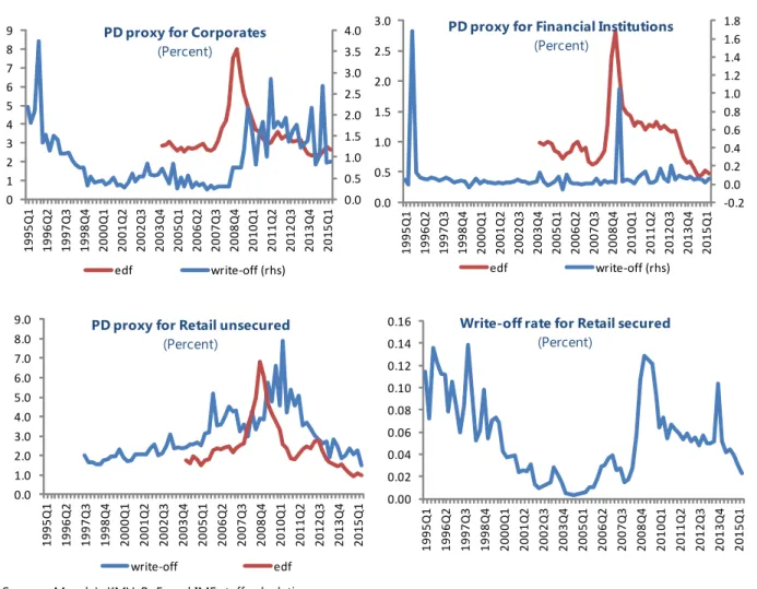
23. For U.K. exposures, the FSAP team applied two different PD proxies to forecast
expected losses. The first PD proxy was obtained from Moody’s Analytics using the average one-year
expected default frequency (EDF) for the corporate group, the financials group, and the consumer nondurables and services group. These categories were mapped to corporate exposures, exposures to institutions,19 and retail unsecured exposures, respectively. The PD proxy for exposures to sovereign and central banks was extracted from sovereign yields. The second PD proxy was sourced from the BoE using write-off rates on U.K. exposures, mainly booked in the U.K., by main asset class.20 Although the write-off rate is the closest measure to estimated portfolio loss ratio, write-off rates tend to lag defaults as defaulted exposures, and loan loss provisions remain on the books for up to about 24 months. Figure 5 shows the difference in the loss distribution across EDFs and write-off rates for selected portfolios.21 While the write-off rate distribution shows positive skew, the EDF distribution is more neutral, with a higher spike and lower persistence, reflecting shifts to expectations at the time of deteriorating economies’ conditions. Appendix I Table 1 summarizes the key variables used to inform PD projections for U.K. exposures.
24. For overseas exposures, the FSAP team applied a market-based PD proxy. The BoE
publishes aggregate write-off rates for U.K. banks’ domestic exposures, but similar data for
18 Data on write-offs by asset class were provided by the BoE on U.K. exposures, which are mainly booked in the U.K.
19 In the IRB advanced approach, almost all exposures to institutions are exposures to financial institutions. See, for
instance, Table 25 in HSBC Holdings plc’s 2014 Pillar 3 disclosures.
20 The PRA considers the write-off rate to be a suitable proxy for the loss rate pending the availability of annual loss
rates collected on a uniform basis through Common Reporting (COREP).
border exposures at the portfolio level are not available. Instead, the FSAP team used Moody’s Analytics one-year EDF for the corporate group, the financials group, the consumer nondurables and services group, and the construction group for Canada, China, France, Germany, Hong Kong SAR, India, Ireland, Italy, Korea, the Netherlands, Singapore, South Africa, Spain, and the U.S.22
25. An integrated credit risk approach drawing on bilateral and multivariate vector
autoregressive (VAR) estimation techniques and nonlinear principal component analysis (PCA)
was used to project conditional PDs. The simultaneous behavior of credit risk, macroeconomic
conditions, financial conditions, and real estate conditions was modeled explicitly in the econometric specification. In addition, global conditions and spillovers from relevant geographies were included as a factor, given the size and prominence of major U.K. banks in international markets.
26. A battery of over 900 credit risk specifications was run to obtain PD projections. The
FSAP team ran a comprehensive set of over 700 bilateral VARs for all pairs of credit risk by PD proxy, asset class, and geography against each variable forecast in the macroeconomic scenario. In addition, 150 PCA analyses were conducted for each factor, PD proxy, asset class, and geography, which fed into 50 multivariate VARs for each PD proxy, asset class, and geography.23 Appendix I gives the details of the econometric approach used to project credit risk.
27. Credit risk in U.K. exposures is mainly driven by financial conditions. Figure 6 shows that
rising spreads across money and equity markets (PC1_fin), and tight corporate credit markets (PC1_fin_c) contribute to rising corporate EDFs with a peak reached in 2017:Q2 at 5.4 percent.
Whereas macro conditions are not statistically significant, an abrupt correction in the commercial real estate (CRE) market is also a driver of heightened credit risk. Write-off rates in U.K. mortgages
increase with deteriorating financial conditions in secured lending markets (PC1_fin_m). Deteriorating macroeconomic conditions are also relevant to explain losses in banks’ mortgage books, whereas movements in housing prices are not statistically significant.
22 Brazil has some materiality mainly for HSBC Holdings plc. However, on August 3, 2015, HSBC Holdings plc
announced that it is selling its entire business in Brazil, comprising HSBC Bank Brazil S.A., to Bradesco for a
consideration of USD 5.2 billion. The sale of HSBC Brazil represents a significant step in HSBC Holding plc’s stated goal to optimize its global network and reduce complexity.
23 For the U.K., over 170 bilateral VARs were estimated linking 2 PD proxies (i.e., EDF and write-off rate) over 4 asset
classes and 24 key variables. For each overseas exposure over 14 countries, 40 bilateral VARs were estimated regressing EDFs over 3 asset classes and 14 variables (7 country-specific, 7 global variables). In addition, 24 PCAs for the United Kingdom (3 factors, 4 asset classes, 2 proxies) and 126 PCAs for overseas exposures (14 geographies, 3 factors, 3 asset classes) were conducted, and a total of 50 multivariate VARs were run.
Figure 4. United Kingdom: Credit Risk and Risk Weights for the U.K. Banking System
Credit risk represents the largest regulatory capital
requirement of U.K. banks…. …most of the credit risk exposures follow the IRB approach for all banks.
While exposures to sovereign and central banks are significant, most of the STA exposures are to the private sector…
…with a 74 percent asset-weighted risk density relative to 5 percent risk density for sovereign and central bank STA exposures.
Asset quality has improved as shown by lower NPL ratios while coverage ratios have edged up…
…reflected in lower market-based measures of bank risk (CDS) while regulatory risk density has increased relative to the crisis period.
Sources: Pillar 3 Disclosures, Bloomberg, and IMF staff calculations.
Note: The bottom two charts show asset-weighted averages for the largest five U.K. banks. 0 100 200 300 400 500 600 700 800 900 RWAs (bn GBP)
Operational risk Market risk CCR Credit risk 0 200 400 600 800 1,000 1,200 1,400
1,600 Credit risk EAD
(bn GBP) STA IRB 0 50 100 150 200 250 300 350 400 EAD STA (bn GBP) other gov&cb 0% 20% 40% 60% 80% 100% HSBC Barclays RBS SC Lloyds Nationwide
Risk weight density STA (in percent) other gov&cb 0.0 10.0 20.0 30.0 40.0 50.0 60.0 70.0 80.0 90.0 0.0 1.0 2.0 3.0 4.0 5.0 6.0 7.0 Asset quality (in percent) npl cov (rhs) 0 50 100 150 200 250 300 0.0 5.0 10.0 15.0 20.0 25.0 30.0 35.0 40.0 45.0 2005Q 1 2005Q 4 2006Q 3 2007Q 2 2008Q 1 2008Q 4 2009Q 3 2010Q 2 2011Q 1 2011Q 4 2012Q 3 2013Q 2 2014Q 1 2014Q 4
Risk of bank assets
Figure 5. United Kingdom: Probability of Default and Credit Loss Rate Across Asset Classes
(In percent)
Sources: Moody's KMV, BoE, and IMF staff calculations.
28. The determinants of credit risk in overseas exposures differ across geographies.
Figure 7 shows the key PD drivers for selected corporate exposures in France and China. While domestic macroeconomic conditions and real estate prices are drivers of corporate credit risk in France,24 global financial conditions, particularly related to FX shocks and the steepening of the yield curve—as well as developments in oil markets—are the most significant drivers of corporate credit risk in China.
24 Although they are not statistically significant at the 5 percent level.
0.0 0.5 1.0 1.5 2.0 2.5 3.0 3.5 4.0 0 1 2 3 4 5 6 7 8 9 1995Q 1 1996Q 2 1997Q 3 1998Q 4 2000Q 1 2001Q 2 2002Q 3 2003Q 4 2005Q 1 2006Q 2 2007Q 3 2008Q 4 2010Q 1 2011Q 2 2012Q 3 2013Q 4 2015Q 1
PD proxy for Corporates
(Percent) edf write-off (rhs) 0.0 1.0 2.0 3.0 4.0 5.0 6.0 7.0 8.0 9.0 1995Q 1 1996Q 2 1997Q 3 1998Q 4 2000Q 1 2001Q 2 2002Q 3 2003Q 4 2005Q 1 2006Q 2 2007Q 3 2008Q 4 2010Q 1 2011Q 2 2012Q 3 2013Q 4 2015Q 1
PD proxy for Retail unsecured
(Percent) write-off edf 0.00 0.02 0.04 0.06 0.08 0.10 0.12 0.14 0.16 1995Q 1 1996Q 2 1997Q 3 1998Q 4 2000Q 1 2001Q 2 2002Q 3 2003Q 4 2005Q 1 2006Q 2 2007Q 3 2008Q 4 2010Q 1 2011Q 2 2012Q 3 2013Q 4 2015Q 1
Write-off rate for Retail secured
(Percent) -0.2 0.0 0.2 0.4 0.6 0.8 1.0 1.2 1.4 1.6 1.8 0.0 0.5 1.0 1.5 2.0 2.5 3.0 1995Q 1 1996Q 2 1997Q 3 1998Q 4 2000Q 1 2001Q 2 2002Q 3 2003Q 4 2005Q 1 2006Q 2 2007Q 3 2008Q 4 2010Q 1 2011Q 2 2012Q 3 2013Q 4 2015Q 1
PD proxy for Financial Institutions
(Percent)
Figure 6. United Kingdom: Aggregate PD Proxy Projections—Selected U.K. Exposures
The first principal component (PC1_Macro) reflects a deteriorating macroeconomic environment characterized by low growth, high inflation, and high unemployment.
The first principal component (PC1_Fin) captures financial turmoil, featuring rising LIBOR rates, GBP depreciation, and a U.K. stock market correction.
U.K. corporate EDF (first column) rises with deteriorating macroeconomic conditions, financial turmoil, and a correction in the CRE segment.
Write-off rates for U.K. mortgages (first column) increase with adverse macroeconomic conditions and tight credit conditions; but are less sensitive to a housing price correction.
Projections of U.K. corporate EDF peak in 2017:Q2 at
5.4 percent… …while write-off rates for U.K. mortgages peak in 2017:Q1 at 0.08 percent, twofold baseline rate levels.
Source: IMF staff estimates.
Cumulative Cumulative Number Value Difference Proportion Value Proportion
1 1.899 1.217 0.633 1.899 0.633
2 0.682 0.263 0.227 2.581 0.860
3 0.419 --- 0.140 3.000 1.000
Eigenvectors (loadings):
Variable PC 1_Macro PC 2 _Macro PC 3 _Macro
UK_G -0.512 0.858 0.049
UK_INF 0.612 0.323 0.722
UK_U 0.604 0.399 -0.690
Cumulative Cumulative Number Value Difference Proportion Value Proportion
1 1.428 0.338 0.476 1.428 0.476
2 1.089 0.607 0.363 2.517 0.839
3 0.483 --- 0.161 3.000 1.000
Eigenvectors (loadings):
Variable PC 1_Fin PC 2_Fin PC 3_Fin LIBOR_GBP 0.079 0.918 0.389
UK_FX 0.691 -0.331 0.643
UK_EQUITY -0.719 -0.218 0.660
EDF_CORP PC1_MACRO PC1_FIN PC1_FIN_c UK_CRE EDF_CORP(-1) 0.572 0.148 0.084 -0.172 2.936 [ 4.286] [ 1.151] [ 0.871] [-0.718] [ 2.913] PC1_MACRO(-1) 0.087 0.913 -0.093 0.100 -1.559 [ 1.201] [ 13.036] [-1.763] [ 0.769] [-2.840] PC1_FIN(-1) 0.114 0.105 0.943 0.133 -1.028 [ 2.912] [ 2.805] [ 33.269] [ 1.894] [-3.489] PC1_FIN_c(-1) 0.125 -0.143 -0.158 0.876 -2.830 [ 1.55] [-1.854] [-2.709] [ 6.076] [-4.666] UK_CRE(-1) -0.024 -0.013 0.008 -0.003 0.881 [-2.152] [-1.246] [ 1.029] [-0.133] [ 10.656] C 1.481 -0.440 -0.340 0.586 -9.452 [ 3.226] [-0.994] [-1.019] [ 0.711] [-2.725] R-squared 0.874 0.925 0.976 0.692 0.929 Adj. R-squared 0.859 0.916 0.973 0.653 0.920
W_MOR PC1_MACRO PC1_FIN_m UK_HOUSING W_MOR(-1) 0.426 -31.173 -84.643 257.798 [ 4.644] [-2.381] [-3.706] [ 2.945] PC1_MACRO(-1) 0.002 0.897 0.203 -0.317 [ 3.372] [ 11.121] [ 1.444] [-0.587] PC1_FIN_m(-1) 0.001 -0.038 0.864 0.177 [ 2.631] [-0.806] [ 10.542] [ 0.562] UK_HOUSING(-1) 0.000 -0.041 -0.027 1.067 [-1.272] [-3.443] [-1.311] [ 13.495] C 0.006 0.604 0.971 -3.022 [ 5.307] [ 3.735] [ 3.443] [-2.795] R-squared 0.868 0.936 0.753 0.913 Adj. R-squared 0.857 0.931 0.734 0.906 0.0 1.0 2.0 3.0 4.0 5.0 6.0 7.0 8.0 9.0 2004Q 1 2005Q 1 2006Q 1 2007Q 1 2008Q 1 2009Q 1 2010Q 1 2011Q 1 2012Q 1 2013Q 1 2014Q 1 2015Q 1 2016Q 1 2017Q 1 2018Q 1 2019Q 1 2020Q 1 edf_corp_b edf_corp_a 0.00 0.02 0.04 0.06 0.08 0.10 0.12 0.14 0.16 1995Q 1 1996Q 3 1998Q 1 1999Q 3 2001Q 1 2002Q 3 2004Q 1 2005Q 3 2007Q 1 2008Q 3 2010Q 1 2011Q 3 2013Q 1 2014Q 3 2016Q 1 2017Q 3 2019Q 1 2020Q 3 baseline adverse
Figure 7. United Kingdom: Aggregate PD Proxy Projections—Selected Cross-Border Exposures
In France, favorable financial conditions transmitted through the current account channel, (low short-term rates, currency depreciation, and upward sloping yield curve) are captured by a high value of PC1_FRA…
…whereas, in China, distress in debt markets transmitted through the capital account channel (duration shocks, depreciation) are reflected in a low value of PC1_CHI.
France corporate EDF (first column) rises with deteriorating macroeconomic conditions, tight financial conditions, and a correction in real estate markets.
China corporate EDF (first column) rises with deteriorating
macroeconomic conditions, stress in the capital account, a correction in U.S. equity markets, and rising oil prices.
Projections of France corporate EDF peak in 2017:Q3 at
6.4 percent… …while China corporate EDF peaks in 2018:Q1 at 8.0 percent.
Source: IMF staff estimates.
Cumulative Cumulative Number Value Difference Proportion Value Proportion
1 1.878 0.942 0.626 1.878 0.626
2 0.936 0.749 0.312 2.814 0.938
3 0.186 --- 0.062 3.000 1.000
Eigenvectors (loadings):
Variable PC 1 _FRA PC 2 _FRA PC 3 _FRA FRA_FX 0.263 0.964 -0.031 FRA_SLOPE 0.685 -0.163 0.710 FRA_ST -0.680 0.208 0.703
Cumulative Cumulative
Number Value Difference Proportion Value Proportion
1 1.505 0.461 0.502 1.505 0.502
2 1.044 0.592 0.348 2.548 0.850
3 0.452 --- 0.151 3.000 1.000
Eigenvectors (loadings):
Variable PC 1 _CHI PC 2_CHI PC 3_CHI
CHI_SLOPE 0.661 -0.385 0.644
CHI_FX 0.214 0.919 0.331
CHI_ST -0.719 -0.081 0.690
FRA_CORP FRA_MACRO FRA_FIN FRA_RE US_EQUITY FRA_CORP(-1) 0.797 0.090 -0.039 0.158 0.880 [ 10.958] [ 1.3458] [-0.830] [ 3.011] [ 0.77714] FRA_MACRO(-1) 0.163 0.855 0.053 -0.193 -3.659 [ 1.772] [ 10.084] [ 0.902] [-2.906] [-2.560] FRA_FIN(-1) -0.130 -0.099 0.909 0.015 0.194 [-1.305] [-1.075] [ 14.323] [ 0.204] [ 0.126] FRA_RE(-1) -0.133 0.074 -0.160 0.984 0.226 [-1.608] [ 0.970] [-3.038] [ 16.529] [ 0.176] US_EQUITY(-1) 0.000 0.015 -0.005 0.019 0.781 [ 0.027] [ 2.423] [-1.246] [ 3.975] [ 7.661] C 0.541 -0.340 0.179 -0.545 0.484 [ 2.066] [-1.408] [ 1.069] [-2.886] [ 0.119] R-squared 0.883 0.870 0.936 0.937 0.760
CHI_CORP CHI_MACRO CHI_FIN US_EQUITY OIL_G CHI_CORP(-1) 0.729 -0.048 0.038 -2.346 -4.767 [ 7.089] [-1.268] [ 0.625] [-1.280] [-2.176] CHI_MACRO(-1) 0.311 0.874 -0.195 -5.175 4.193 [ 1.595] [ 12.25] [-1.720] [-1.491] [ 1.011] CHI_FIN(-1) 0.237 -0.068 0.876 -0.855 -0.765 [ 2.291] [-1.803] [ 14.52] [-0.464] [-0.347] US_EQUITY(-1) -0.008 0.004 0.002 0.829 0.192 [-1.331] [ 1.835] [ 0.432] [ 7.506] [ 1.452] OIL_G(-1) 0.008 -0.002 -0.004 -0.110 0.836 [ 2.169] [-1.708] [-1.933] [-1.640] [ 10.46] C 0.756 0.027 -0.084 5.996 10.971 [ 2.665] [ 0.261] [-0.506] [ 1.186] [ 1.816] R-squared 0.689 0.899 0.948 0.750 0.844 0 1 2 3 4 5 6 7 8 9 2002Q 2 2003Q 2 2004Q 2 2005Q 2 2006Q 2 2007Q 2 2008Q 2 2009Q 2 2010Q 2 2011Q 2 2012Q 2 2013Q 2 2014Q 2 2015Q 2 2016Q 2 2017Q 2 2018Q 2 2019Q 2 2020Q 2 FRA_CORP_b FRA_CORP_a 0 1 2 3 4 5 6 7 8 9 2002Q 2 2003Q 2 2004Q 2 2005Q 2 2006Q 2 2007Q 2 2008Q 2 2009Q 2 2010Q 2 2011Q 2 2012Q 2 2013Q 2 2014Q 2 2015Q 2 2016Q 2 2017Q 2 2018Q 2 2019Q 2 2020Q 2 CHI_CORP_b CHI_CORP_a
29. To avoid a structural shift at the cut-off date between banks’ estimated PDs and FSAP team’s PD projections, an econometric approach drawing on banks’ Pillar 3 disclosures was
used. Table 1 shows an extract from HSBC Holdings plc’s Pillar 3 disclosures. The choice of HSBC is
motivated by the size of the firm’s balance sheet (HSBC Holdings plc accounts for one-third of U.K. major banks’ assets), its broad product base, and its geographic footprint. Notwithstanding caveats related to changes in the composition of the underlying portfolios, the peak of bank estimated PDs stood at 4 percent for European unsecured retail exposures, 15 percent for the U.S. mortgage portfolio,25 and 3 percent for both European mortgage exposures and global corporate exposures. On the other hand, PDs for exposures to institutions (mainly financial) stood at 0.5 percent at the height of the financial crisis, whereas the average PD for sovereign exposures peaked at 0.2 percent in 2008.
30. The forecast path of conditional PD proxies under the macroeconomic scenario is
transformed using information embedded in bank estimated PDs, adjusting for point-in-time
(PiT) parameters. There are two key reasons PD proxies and bank-specific PDs are likely to differ.
First, PD proxies are calculated for the aggregate market portfolio, and hence do not necessarily reflect the underlying risk profile of banks’ portfolios. Second, forecast PD proxies are either market-based (using the Merton approach) or approximate the ex post realization of credit losses (write-off rates). By contrast, bank-estimated PDs are ex ante measures computed using banks’ approved IRB models for the calculation of capital requirements. For consistency with the PRA regulatory regime, the time series of bank-specific PDs by asset class and geography is regressed on the historical series of EDFs and write-off rates. The estimated coefficients were used to forecast bank-specific PDs over the stress test horizon. Figure 8 shows the aggregate PD proxies and bank-estimated PDs for selected U.K. portfolios. To compute expected losses, an adjustment to bank-specific PD projections is performed to account for the cyclicality of PiT parameters under the adverse scenario.
where j
t i
PD
, is bank i blended PD for portfolio j (that is, including both defaulted and non-defaulted counterparties) at time t, and jt PD
is the aggregate PD shift for portfolio j at time t.
25 HSBC Holdings plc's has a significant exposure to the U.S. subprime market followed by its acquisition of U.S.
lender Household Finance.
j j j t t i t i
PD
PD
PD
1 , ,Table 1. United Kingdom: Bank-Estimated PDs for IRB Exposures
Source: HSBC Holdings plc Pillar 3 disclosures over 2008–15 and IMF staff calculations. Note: For 2013–15, the data is for Asia (no split between HK and Rest of Asia).
Approach to LGD
Calculation of LGD for U.K. mortgages
31. The FSAP team applied a
fair-value option approach to compute LGDs
for mortgages. The estimated LGD on
mortgages has option-like features
conditional on the original LTV distribution and housing prices at default. LGD is a highly nonlinear function of the house price at the time of default VT and the original LTVt ratio (priced at the time of origination t) of the mortgage loan (see chart). This
warrants the estimation of the initial distribution of LTV by vintage repriced at stressed house prices rather than relying on original LTV ratios. VT LGDT LTVt=100% LTVt=80% LTVt=60% 100 80 60 60 80 100
LGD and House Prices
LGDTshows the LGD at the time of default T, LTVt reflects the original LTV distribution at time t, and VT denotes the house price at the time of default T.
2008 2009 2010 2011 2012 2013 2014 2015
Retail (by region) Europe PD mortgages 1.51 1.67 1.53 1.00 0.92 3.08 0.98 1.43 PD unsecured 3.91 4.01 3.47 2.57 1.98 2.06 1.65 1.56 HK1 PD mortgages 1.15 0.81 0.76 0.75 0.50 3.06 1.00 0.99 PD unsecured 1.71 1.86 1.52 1.36 0.94 1.14 1.21 1.24 Rest of Asia PD mortgages 2.06 2.05 1.55 1.47 1.37 3.06 1.00 0.99 PD unsecured 0.50 0.60 0.50 0.50 0.50 1.14 1.21 1.24 North America PD mortgages 10.27 13.39 12.92 14.65 15.01 8.48 11.54 9.66 PD unsecured 10.48 9.18 6.28 4.90 5.72 3.30 5.37 4.38
Wholesale IRB Foundation
PD gov and central banks 0.20 0.16 0.11 0.11 0.13 0.17 0.17 0.14
PD institutions 0.47 0.49 0.36 0.46 0.39 0.46 0.36 0.18