The Longitudinal Study of Australian Children
Annual statistical report 2010
© Commonwealth of Australia 2011
This work is copyright. Apart from any use as permitted under the Copyright Act 1968, no part may be reproduced by any process without prior written permission from the Commonwealth Copyright Administration, Attorney-General’s Department, 3–5 National Circuit, Barton ACT 2600 or posted at <www.ag.gov.au/cca>.
The Australian Institute of Family Studies is committed to the creation and dissemination of research-based information on family functioning and wellbeing. Views expressed in its publications are those of individual authors and may not reflect those of the Australian Institute of Family Studies. Growing Up in Australia: The Longitudinal Study of Australian Children is conducted in partnership between the Australian Government Department of Families, Housing, Community Services and Indigenous Affairs (FaHCSIA), the Australian Institute of Family Studies (AIFS) and the Australian Bureau of Statistics (ABS), with advice provided by a consortium of leading researchers from research institutions and universities throughout Australia. Australian Institute of Family Studies. (2011). The Longitudinal Study of Australian Children Annual Statistical Report 2010
Bibliography. Edited by Brigit Maguire
Copyedited by Kelly Robinson and Lan Wang Typeset by Lan Wang
Foreword xi
Acknowledgements xiii
Glossary of LSAC terms
xv
1 Introduction
1
1.1 About the study 2
1.2 Analyses presented in this report 4
1.3 Notes 4
1.4 Further reading 5
1.5 References 5
2 Characteristics of the children and their families
7
Brigit Maguire, Australian Institute of Family Studies
2.1 The children 8
2.2 Parent characteristics 8
2.3 Family characteristics 11
2.4 Family cultural and language background 14
2.5 Further reading 17
2.6 References 17
3 How family composition changes across waves
19
Brigit Maguire, Australian Institute of Family Studies
3.1 Children’s parents 19
3.2 Children’s families 24
3.3 Change in the residents of children’s households 26
3.4 Summary 26
3.5 Further reading 27
3.6 References 27
4 Parents and the labour market
29
Matthew Gray and Jennifer Baxter, Australian Institute of Family Studies
4.1 Parental employment 29
4.2 Children growing up in jobless families or families with part-time only employment 32 4.3 Relationship between parental joblessness and child wellbeing 35
4.4 Parental employment and family wellbeing 37
4.5 Summary 39
4.6 Further reading 40
4.7 References 41
5 Parenting practices and behaviours
43
Nina Lucas, Murdoch Childrens Research Institute
Jan M. Nicholson, Murdoch Childrens Research Institute and the Parenting Research Centre Brigit Maguire, Australian Institute of Family Studies
5.1 Parenting measures 44 5.2 Descriptive statistics 46 5.3 Sub-group analyses 48 5.4 Summary 54 5.5 Further reading 54 5.6 References 55
6 Children’s experiences of child care
57
Linda J. Harrison, Charles Sturt University6.1 Definitions 57
6.2 How many 0–1 year olds and 2–3 year olds received child care? Why was care used
or why not? 58
6.3 Type(s) of child care experienced by 0–1 year olds and 2–3 year olds 59 6.4 Quantity of child care experienced by 0–1 year olds and 2–3 year olds 60 6.5 Multiplicity of child care experienced by 0–1 year olds and 2–3 year olds 60 6.6 Types of child care experienced by 0–1 year olds and 2–3 year olds in different family
circumstances 61
6.7 Summary 67
6.8 Further reading 68
6.9 References 68
7 Family education environment
71
Suzanne MacLaren, Australian Institute of Family Studies
7.1 Helping with homework 72
7.2 Involvement in class activities 72
7.3 Mother’s expectations of child’s future educational achievements 74
7.4 Reading to child 76
7.5 Number of children’s books in the home 76
7.6 Television in child’s bedroom 77
7.7 Time spent watching television 78
7.8 Summary 78
7.9 Further reading 79
7.10 References 79
8 A longitudinal view of children living in disadvantaged neighbourhoods
81
Ben Edwards, Australian Institute of Family Studies8.1 Neighbourhood socio-demographic characteristics 82
8.2 Children’s experiences over time of living in disadvantaged neighbourhoods 83 8.3 Changes in neighbourhood socio-economic status over the waves: Changes in the
neighbourhood or residential mobility? 85
8.4 Summary 87
8.5 Further reading 88
8.6 References 88
9 How young children are faring: Behaviour problems and competencies
91
Diana Smart, Australian Institute of Family Studies9.1 Prevalence of behaviour problems at 2–3 years 92
9.2 Competencies at 2–3 years 96
9.3 Summary of trends at 2–3 years 98
9.4 Prevalence of behaviour problems at 4–5 years 99
9.5 Competencies at 4–5 years 104
9.6 Summary of trends at 4–5 years 105
9.7 Summary 106
9.8 Further reading 106
Brigit Maguire, Australian Institute of Family Studies
Stephen R. Zubrick, Curtin Health Innovation Research Institute and the Telethon Institute for Child Health Research
10.1 Language assessments: Waves 1–3 107
10.2 B cohort 108
10.3 K cohort 115
10.4 Key findings and future opportunities 121
10.5 Further reading 121
10.6 References 121
11 Children’s pre- and perinatal health experiences
123
Brigit Maguire, Australian Institute of Family Studies
11.1 Who provides mothers with medical care during their pregnancy? 124
11.2 What medications do mothers take during pregnancy? 125
11.3 What medical conditions do mothers experience during pregnancy? 127 11.4 How many mothers report drinking alcohol or smoking cigarettes during pregnancy? 128 11.5 Which mothers had a pre-term birth or a child with a low birth weight? 130
11.6 Summary 131
11.7 Further reading 132
List of figures
Figure 2.1 Distribution of B cohort, by child’s age, Wave 1 8 Figure 2.2 Distribution of K cohort, by child’s age, Wave 1 8 Figure 2.3 Distribution of age of biological mothers at birth of study child, B and K cohorts 9 Figure 2.4 Distribution of age of biological fathers at birth of study child, B and K cohorts 9 Figure 2.5 Education levels of children’s mothers, B and K cohorts, Wave 1 10 Figure 2.6 Highest level of education between children’s parents, B and K cohort, Wave 1 11 Figure 2.7 Distribution of children, mothers and fathers who identified as Aboriginal or Torres
Strait Islander, B and K cohorts, Wave 1 17 Figure 3.1 Distribution of age of lone mothers at birth of study child, as a proportion of all
mothers in age group, B and K cohorts, Waves 1–3 22 Figure 3.2 Children with a new sibling born since the previous wave, B and K cohorts, Waves 2 and 3 25 Figure 3.3 Distribution of children who had a change in the household since the previous wave,
B and K cohorts, Waves 2 and 3 27
Figure 4.1 Total weekly hours worked by parents in two-parent families, by age of youngest child,
B and K cohorts, Waves 1–3 32
Figure 4.2 Child outcome indices at Wave 3, by joblessness over Waves 1–3, B cohort 36 Figure 4.3 Child outcome indices at Wave 3, by joblessness over Waves 1–3, K cohort 36 Figure 4.4 Mothers feeling rushed or pressed for time, by age of youngest child and weekly work
hours, B and K cohorts, Waves 1–3 38
Figure 4.5 Employed mothers missing out on family activities due to work, by age of youngest
child and weekly work hours, B and K cohorts, Waves 1–3 38 Figure 4.6 Fathers feeling rushed or pressed for time, by age of youngest child and weekly work
hours, B and K cohorts, Waves 1–3 39
Figure 4.7 Employed fathers missing out on family activities due to work, by age of youngest
child and weekly work hours, B and K cohorts, Waves 1–3 39 Figure 4.8 Difficulty of life at present for mothers and fathers, by weekly work hours,
B and K cohorts, Waves 1–3 40
Figure 7.1 Average weekly hours spent watching television, K cohort Wave 1 and B cohort Wave 3 78 Figure 8.1 Between-wave neighbourhood mobility, by neighbourhood disadvantage in the
previous wave, B and K cohorts, Waves 1–3 87 Figure 9.1 Comparison of 2–3 year old subgroups on total behaviour problems, BITSEA scale
(mothers’ reports), B cohort, Wave 2 94 Figure 9.2 Comparison of 2–3 year old sub-groups on the total number of competencies, BITSEA
scale (mothers’ reports), B cohort, Wave 2 97 Figure 9.3 Cohort mean scores on SDQ behaviour problem scales (mothers’ reports), B cohort, Wave 3 99 Figure 9.4 Comparison of boys and girls on SDQ behaviour problem scales at 4–5 years
(mothers’ reports), B cohort, Wave 3 101 Figure 9.5 Comparison of children from families differing on socio-economic position on SDQ
behaviour problem scales at 4–5 years (mothers’ reports), B cohort, Wave 3 103 Figure 9.6 Comparison of 4–5 year old children with differing numbers of siblings on SDQ
behaviour problem scales (mothers’ reports), B cohort, Wave 3 103 Figure 9.7 Comparison of 4–5 year old children from metropolitan and regional areas on SDQ
behaviour problem scales (mothers’ reports), B cohort, Wave 2 103 Figure 9.8 Comparison of 4–5 year old subgroups on SDQ prosocial behaviour scale (mothers’
reports), B cohort, Wave 3 105
Figure 11.1 Mothers who reported taking prescription medications during pregnancy (n = 5,097),
B cohort, Wave 1 126
Figure 11.2 Mothers who reported taking over-the-counter medications during pregnancy
Table 1.1 Number of children, B and K cohorts, Waves 1–3 2 Table 1.2 Response rates, B and K cohorts, Waves 1–3 4 Table 2.1 Characteristics and categories of subpopulation groups 7 Table 2.2 Distribution of mothers and fathers working full-time, part-time or not currently
working, B and K cohorts, Waves 1–3 11 Table 2.3 Distribution of children, by whether living in two-parent or lone-mother families,
B and K cohorts, Waves 1–3 12
Table 2.4 Distribution of children by Australian state/territory, B and K cohorts, Waves 1–3 12 Table 2.5 Distribution of children, by metropolitan and regional areas, B and K cohorts, Waves 1–3 12 Table 2.6 Distribution of weighted data across SEP categories, B and K cohorts, Waves 1–3 13 Table 2.7 Distribution of children with no, one, two or three or more siblings in the home,
B and K cohorts, Waves 1–3 14
Table 2.8 Distribution of country/region of birth, by study child, their mother and their father,
B and K cohorts 14
Table 2.9 Ten most common countries of birth, by mothers and fathers, B and K cohorts 15 Table 2.10 Distribution of age on arrival in Australia, children’s parents, B and K cohorts 15 Table 2.11 Main language spoken at home, by study child, their mother and their father,
B and K cohorts, Wave 1 16
Table 2.12 Main language spoken at home (English or non-English), by study child, their mother
and their father, B and K cohorts, Waves 1–3 16 Table 3.1 Distribution of children living in three major family types, B and K cohorts, Waves 1–3 20 Table 3.2 Change in family type, B cohort, Waves 1 and 3 21 Table 3.3 Change in family type, K cohort, Waves 1 and 3 22 Table 3.4 Parents’ relationship status, B and K cohorts, Waves 1–3 23 Table 3.5 Change in parents’ relationship status, B cohort, Waves 1 and 3 24 Table 3.6 Change in parents’ relationship status, K cohort, Waves 1 and 3 24 Table 3.7 Distribution of children living with different types of siblings, B and K cohorts, Waves 1–3 25 Table 3.8 Distribution of parents with children living elsewhere, B and K cohorts, Waves 1–3 26 Table 4.1 Paid employment of mothers with an infant aged 3–14 months old, B cohort, Wave 1 30 Table 4.2 Mother’s employment status and hours of paid work, by age of youngest child, B and
K cohorts, Waves 1–3 30
Table 4.3 Fathers’ employment status and hours of paid work, by age of youngest child,
B and K cohorts, Waves 1–3 31
Table 4.4 Family labour supply in lone- and two-parent families, by age of youngest child,
B and K cohorts, Waves 1–3 33
Table 4.5 Persistence of joblessness, by family type, B and K cohorts, Waves 1–3 34 Table 4.6 Proportion of mothers and fathers with low level of educational attainment
(incomplete secondary education), by family joblessness and family type, K cohort,
Waves 1–3 35
Table 5.1 Descriptive statistics of parenting scores at each wave, B cohort, Waves 1–3 47 Table 5.2 Descriptive statistics of parenting scores at each wave, K cohort, Waves 1–3 47 Table 5.3 Poor parenting outcomes, by population subgroups, B cohort mothers, Waves 1–3 50 Table 5.4 Poor parenting outcomes, by population subgroups, B cohort fathers, Waves 1–3 51 Table 5.5 Poor parenting outcomes, by population subgroups, K cohort mothers, Waves 1–3 52 Table 5.6 Poor parenting outcomes, by population subgroups, K cohort fathers, Waves 1–3 53 Table 6.1 Type of child care received (0–1 year olds and 2–3 year olds), B cohort, Waves 1 and 2 59 Table 6.2 Type of child care, by weekly hours (quantity) of care (for children receiving care),
B cohort, Waves 1 and 2 60
Table 6.3 Type of child care, by number of weekly care arrangements (for children receiving
Table 6.4 Type and quantity of child care received, by family socio-economic position (for all
children), B cohort, Waves 1 and 2 62 Table 6.5 Type and quantity of child care received, by mothers’ work hours (full-time, part-time,
not currently working), B cohort, Waves 1 and 2 64 Table 6.6 Type and quantity of child care received, by geographic location, B cohort, Waves 1 and 2 65 Table 6.7 Type and quantity of child care received, by language spoken at home, B cohort,
Waves 1 and 2 65
Table 6.8 Type and quantity of child care received, by number of children in the household,
B cohort, Waves 1 and 2 66
Table 7.1 Frequency with which mothers helped children with homework, by family
socio-economic position, K cohort, Waves 2 and 3 72 Table 7.2 Frequency with which mothers helped children with homework, by family type,
K cohort, Waves 2 and 3 73
Table 7.3 Mother’s involvement in class activities during the previous school term, by family
socio-economic position, K cohort, Waves 2 and 3 73 Table 7.4 Mothers’ involvement in class activities during the previous school term, by main
language spoken at home by mother, K cohort, Waves 2 and 3 73 Table 7.5 Mothers’ expectations of child’s educational achievements, by highest level of
parental education, K cohort, Waves 2 and 3 74 Table 7.6 Mothers’ expectations of child’s educational achievements, by mother’s age at birth of
child, K cohort, Waves 2 and 3 75
Table 7.7 Frequency with which child is read to, by highest level of parental education (both
Parent 1 and Parent 2), K cohort Wave 1 and B cohort Wave 3 76 Table 7.8 Frequency with which child is read to, by mother’s age at birth of child, K cohort Wave
1 and B cohort Wave 3 77
Table 7.9 Number of children’s books in the home, by family socio-economic position, K cohort,
Wave 2 77
Table 7.10 Whether child has a television in their bedroom, by family socio-economic position,
K cohort, Wave 2 78
Table 8.1 Neighbourhood social and demographic variables, B and K cohorts, Waves 1–3 82 Table 8.2 Children living in advantaged and disadvantaged neighbourhoods, B and K cohorts,
Waves 1–3 83
Table 8.3 Transitions into and out of living in a disadvantaged neighbourhood, B cohort, Wave 1
to Wave 2 83
Table 8.4 Transitions into and out of living in a disadvantaged neighbourhood, B cohort, Wave 2
to Wave 3 84
Table 8.5 Transitions into and out of living in a disadvantaged neighbourhood, K cohort, Wave 1
to Wave 2 84
Table 8.6 Transitions into and out of living in a disadvantaged neighbourhood, K cohort, Wave 2
to Wave 3 85
Table 8.7 Mobility out of neighbourhood of residence in the previous wave, B and K cohorts,
Waves 1–3 85
Table 8.8 Transitions into and out of living in a disadvantaged neighbourhood between waves
and neighbourhood mobility, B cohort, Waves 1–3 86 Table 8.9 Transitions into and out of living in a disadvantaged neighbourhood between waves
and neighbourhood mobility, K cohort, Waves 1–3 87 Table 9.1 Percentage of children showing differing types of behaviour problems at 2–3 years,
BITSEA scale (mothers’ reports), B cohort, Wave 2 93 Table 9.2 Percentage of children showing differing types of competencies at 2–3 years,
BITSEA scale (mothers’ reports), B cohort, Wave 2 96 Table 9.3 Percentage of children showing differing types of behaviour problems at 4–5 years,
SDQ (mothers’ reports), B cohort, Wave 3 100 Table 9.4 Percentage of children showing prosocial behaviour at 4–5 years, SDQ (mothers’
reports), B cohort, Wave 3 104
groups, B cohort, Wave 1 110 Table 10.4 Percentage of children scoring above and below the 15th percentile for the whole
cohort on the CSBS DP Infant–Toddler Checklist, B cohort, Wave 1 112 Table 10.5 Percentage of parents with concerns about their child’s expressive and receptive
language abilities (PEDS), B cohort, Wave 1 112 Table 10.6 Percentage of children scoring above and below the 15th percentile for the whole
cohort on the Macarthur CDI–3, B cohort, Wave 2 113 Table 10.7 Percentage of parents with concerns about their child’s expressive and receptive
language abilities (PEDS), B cohort, Wave 2 113 Table 10.8 Percentage of children who scored above and below the 15th percentile for the
whole cohort on the Adapted PPVT–lll, B cohort, Wave 3 114 Table 10.9 Teacher ratings of children’s expressive and receptive language skills in relation to
other children of the same age, B cohort, Wave 3 114 Table 10.10 Percentage of children who scored above and below the 15th percentile for the
whole cohort on the PPVT–lll, K cohort, Wave 1 115 Table 10.11 Teacher ratings of children’s expressive and receptive language skills in relation to
other children the same age, K cohort, Wave 1 116 Table 10.12 Percentage of parents with concerns about their child’s expressive and receptive
language abilities (PEDS), K cohort, Wave 1 116 Table 10.13 Percentage of children who scored above and below the 15th percentile for the
whole cohort on the PPVT–lll, K cohort, Wave 2 117 Table 10.14 Percentage of children who scored above and below the 15th percentile on the
CCC-2, K cohort, Wave 2 117
Table 10.15 Teacher ratings of children’s language and literacy skills in relation to other children
of the same age on the ARS: Language and Literacy Scale, K cohort, Wave 2 118 Table 10.16 Percentage of parents with concerns about their child’s expressive and receptive
language abilities (PEDS), K cohort, Wave 2 119 Table 10.17 Percentage of children who scored above and below the 15th percentile for the
whole cohort on the PPVT–lll, K cohort, Wave 3 119 Table 10.18 Teacher ratings of children’s language and literacy skills in relation to other children
of the same age on the ARS: Language and Literacy Scale, K cohort, Wave 3 120 Table 10.19 Teacher ratings of children’s language and literacy skills and academic achievement in
relation to other children at the same grade level, K cohort, Wave 3 121 Table 11.1 Use of antenatal care providers by maternal age at birth, by family SEP and by
residence in metropolitan/regional area, B cohort, Wave 1 125 Table 11.2 Use of prescription and over-the-counter medications during pregnancy, by maternal
age at birth and by family socio-economic position, B cohort, Wave 1 127 Table 11.3 Medical conditions experienced during pregnancy, by maternal age at birth and by
family socio-economic position, B cohort, Wave 1 128 Table 11.4 Percentage of mothers who reported drinking alcohol/smoking cigarettes during
pregnancy, B and K cohorts, Wave 1 129 Table 11.5 Drinking alcohol and cigarette smoking, by maternal age at birth and by family
socio-economic position, B cohort, Wave 1 130 Table 11.6 Gestational age and low birth weight, by maternal age at birth and by family
I am pleased to introduce the first of the Annual Statistical Report series for Growing Up in Australia: The Longitudinal Study of Australian Children (LSAC). This is a new series of reports produced by the Australian Institute of Family Studies that will provide policy-makers, researchers, practitioners and others with a valuable introduction to the wealth of information collected by the study. This report examines the multiple facets of children’s lives that influence their wellbeing, including their family characteristics and their experiences of the broader social environment. Children’s early development is an important precursor for their outcomes in later childhood, adolescence and adulthood. Children’s families form the predominant environment in which early development takes place, and characteristics of their families influence many aspects of their lives. Their experiences within the broader environmental context also interact with their family environments and their developmental outcomes to influence their wellbeing.
Using data from children aged 0–9 years, chapters in the report make use of the study’s longitudinal nature to investigate children’s experiences over time. This provides insight into the experience of prolonged disadvantage and the critical points of transition in children’s lives. Sections of the report examine how experiences and developmental outcomes vary for different demographic groups of children, including children from different socioeconomic backgrounds and different family structures.
The results presented in this report provide a foundation for further research and information that can inform government policies and programs that support the wellbeing of children and their families.
Alan Hayes Director
Australian Institute of Family Studies
Acknowledgements
The Australian Institute of Family Studies thanks the Australian Government Department of Families, Housing, Community Services and Indigenous Affairs (FaHCSIA) for funding this report, and the FaHCSIA LSAC Team for their contributions.
We are also grateful to the following reviewers for their comments on earlier versions of specific chapters:
■ Professor Donna Berthelsen, School of Early Childhood, Queensland University of Technology; ■ Professor Deborah Brennan, Social Policy Research Centre, University of New South Wales; ■ Associate Professor Boyd Hunter, Centre for Aboriginal Economic Policy Research, Australian
National University;
■ Professor Ariel Kalil, Harris School of Public Policy Studies, University of Chicago; ■ Dr Gehan Roberts, Centre for Community Child Health, The Royal Children’s Hospital; ■ Professor Peter Whiteford, Social Policy Research Centre, University of New South Wales; and ■ employees of the Australian Institute of Family Studies, the Australian Institute of Health and
Welfare, the Department of Education, Employment and Workplace Relations, the Department of Health and Ageing, and the Department of Families, Housing, Community Services and Indigenous Affairs.
For more information about the study, see <www.aifs.gov.au/growingup>.
This report uses unit record data from Growing Up in Australia: The Longitudinal Study of Australian Children. The study is conducted in partnership between the Department of Families, Housing, Community Services and Indigenous Affairs, Australian Institute of Family Studies (AIFS), and Australian Bureau of Statistics (ABS). The findings and views reported in this report are those of the individual authors and should not be attributed to FaHCSIA, AIFS or the ABS.
B cohort The younger group (“baby” cohort) of study children. Aged 0–1 in Wave 1 (2004)
Aged 2–3 in Wave 2 (2006) Aged 4–5 in Wave 3 (2008)
K cohort The older group (“kindergarten” cohort) of study children. Aged 4–5 in Wave 1 (2004)
Aged 6–7 in Wave 2 (2006) Aged 8–9 in Wave 3 (2008)
LSAC Growing Up in Australia: The Longitudinal Study of Australian Children. A nationally representative longitudinal study of child development, which commenced in 2004. Data is collected from study children, their parents, carers and teachers, and through linkage with other national datasets.
Parent 1 The child’s primary parent, defined as the child’s primary caregiver, or the parent who knows the child best. In the majority of cases, this is the child’s biological mother, but can also be the father or another guardian.
Parent 2 The child’s second parent, usually the partner of the primary parent. In most cases, this is the child’s biological father, but can also be the mother, another partner of the primary parent, or another guardian.
Study child (or child)
The sampling unit for LSAC is the study child, so “child” refers to the child selected for inclusion in the study. Data collected and reported relates to this child.
Wave Periods of data collection.
Wave 1 occurred in 2004 (B cohort were 0–1 years, K cohort were 4–5 years) Wave 2 occurred in 2006 (B cohort were 2–3 years, K cohort were 6–7 years) Wave 3 occurred in 2008 (B cohort were 4–5 years, K cohort were 8–9 years)
Chapter 1: Introduction
1
Introduction
C
hildren born in the early years of this millennium are growing up in an Australian society different to that experienced by any previous generation. In order to ensure that children growing up in Australia have every chance to experience a happy and healthy start to life, it is essential that policy-makers and researchers have access to quality data about children’s development in the current economic, social and cultural environment. Growing Up in Australia: The Longitudinal Study of Australian Children (LSAC) is Australia’s first nationally representative longitudinal study of child development. The study provides valuable data on children, their families and their wider environments, and enables researchers and policy-makers to understand how these change and interact as children grow up.This is the first volume in the LSAC Annual Statistical Report series. The purpose of these reports is to provide an overview of the data from the study and thereby describe aspects of Australian children’s lives and development. The reports will also be able to provide longitudinal statistics to describe the dynamics of change as children develop, and how their families and lives change as they grow older.
This report is structured around six themes (covering the two broad domains of
children’s environments and children’s development), with chapters as follows: 1. Introduction
Families
2. Characteristics of the children and their families 3. How family composition changes across waves 4. Parents and the labour market
5. Parenting practices and behaviours
Education
6. Children’s experiences of child care 7. Family education environment
Housing, neighbourhood and community
8. A longitudinal view of children living in disadvantaged neighbourhoods
Socio-emotional development
9. How young children are faring: Behaviour problems and competencies
Cognitive development and learning
10. Children’s language development
Physical development and health
Each chapter concludes with a list of “further reading” for those interested in other LSAC work undertaken on particular topics.
The first section of this introductory chapter provides a brief overview of LSAC and the second section describes the analytical approaches used throughout the main chapters.
1.1 About the study
Growing Up in Australia: The Longitudinal Study of Australian Children is Australia’s first nationally representative longitudinal study of child development. The purpose of the study is to provide data that enable a comprehensive understanding of children’s development within Australia’s current social, economic and cultural environment (Department of Families, Housing, Community Services and Indigenous Affairs [FaHCSIA] LSAC Team, 2009). The longitudinal nature of the study enables researchers to examine the dynamics of change as children develop, and to go beyond the static pictures provided by cross-sectional statistics.
The study was initiated and is funded by the Australian Government Department of Families, Housing, Community Services and Indigenous Affairs and is conducted in partnership with the Australian Institute of Family Studies (AIFS) and the Australian Bureau of Statistics (ABS). A consortium of leading researchers and experts from universities and research agencies provide advice to the study.
Study design
The study has an accelerated cross-sequential design, with two cohorts of children:
■ the B (“baby”) cohort, who were aged 0–1 years at the beginning of the study (born from March 2003 to February 2004); and
■ the K (“kindergarten”) cohort, who were aged 4–5 years at the beginning of the study (born from March 1999 to February 2000).
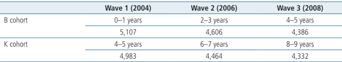
The first wave of data collection was in 2004, with subsequent main waves every two years. Table 1.1 summarises the ages and sample sizes for the two cohorts across the first three waves of the study.
This design means that from the third wave of the study, the children’s ages overlap. That is, children are aged 4–5 years in the first wave for the K cohort and in the third wave for the B cohort. In covering the first three waves of the study, this report includes data on children between the ages of 0 and 9 years.
Table 1.1 Number of children, B and K cohorts, Waves 1–3
Wave 1 (2004) Wave 2 (2006) Wave 3 (2008)
B cohort 0–1 years 2–3 years 4–5 years
5,107 4,606 4,386
K cohort 4–5 years 6–7 years 8–9 years
4,983 4,464 4,332
Respondents and collection methods
A unique feature of LSAC is its use of multiple respondents. This provides a rich picture of children’s lives and development, as responses can be compared between different respondents (e.g., parents and teachers) to provide an insight into children’s behaviour in different contexts. The use of multiple respondents also helps to reduce the effects of respondent bias. In the first three waves of the study, data were collected from:
■ parents of the study child:
– the primary parent (not necessarily a biological parent) (Parent 1)—defined as the person who knows most about the child;
– a parent living elsewhere (PLE)—a parent who lives apart from the child but who has contact with the child);
■ the study child;
■ carers/teachers (depending on child’s age); and ■ interviewer observations.
In the first three waves of the study, the primary respondent was the child’s primary carer. In the majority of cases, this was the child’s biological mother, but may also have been someone else who knew the most about the child.
A variety of data collection methods have been used in the study, including: ■ face-to-face interviews;
■ self-complete questionnaires:
– during interview:
• on paper;
• by computer-assisted interview (CAI); and
• by computed-assisted self-interview (CASI);
– leave-behind (paper); and
– mail-out;
■ physical measurements of the child, including height, weight, girth, body fat, blood pressure; ■ time use diaries;
■ computer-assisted telephone interviews; and ■ linked administrative data (e.g., Medicare).
The interviews and questionnaires include validated scales appropriate to the children’s ages.
Sampling and survey design
The sampling unit for LSAC is the study child. The sampling frame for the study was the Medicare Australia (formerly the Health Insurance Commission) enrolments database, which is the most comprehensive database of Australia’s population, particularly of young children. In 2004, approximately 18,800 children were sampled from this database, using a two-stage clustered design. In the first stage, 311 postcodes were randomly selected (very remote postcodes were excluded due to the high cost of collecting data from these areas). In the second stage, children were randomly selected within each postcode, with the two cohorts sampled from the same postcodes. A process of stratification was used to ensure that the numbers of children selected were roughly proportionate to the total numbers of children within each state/territory, and within the capital city statistical districts and the rest of each state. The method of postcode selection took into account the number of children in the postcode; hence, all the potential participants in the study Australia-wide had an approximately equal chance of selection (about one in 25).1
Response rates
The 18,800 families selected were then invited to participate in the study. Of these, 54% of families agreed to take part in the study (57% of B cohort families and 50% of K cohort families). About 35% of families refused to participate (33% of B cohort families and 38% of K cohort families), and 11% of families could not be contacted (e.g., because the address was out of date, or only a post office box address was provided) (10% of B cohort families and 12% of K cohort families). This resulted in a nationally representative sample of 5,107 0–1 year olds and 4,983 4–5 year olds who were Australian citizens or permanent residents. Table 1.2 presents the response rates for each of the three waves2.
1 See Soloff, Lawrence, & Johnstone (2005) for more information about the study design.
2 The sample size reported in analyses using more than one wave may be lower than shown in Table 1.2 because it includes only those responding to all waves. (Note that some of the families responding in Wave 3 did not respond in Wave 2.)
1.2 Analyses presented in this report
This report includes data from the first three waves of the study. Analyses for the two cohorts (B and K) are presented separately throughout this report.
Given the breadth and depth of topics included in the study, chapters in this report do not necessarily use data from all three waves and/or cohorts. For example, under the Education theme, this report focuses on the first two waves of the study, looking at family child care arrangements. Further examination of later education will be continued in future reports.
Two general approaches are taken to the analyses in this report:
■ comparisons between certain subpopulation groups (introduced in Chapter 2) on the various aspects of children’s environments and development—for example, comparison of parenting behaviours for mothers of different ages; and
■ examination of trends across waves (as children get older)—for example, examination of how patterns of child care change as children get older; or examination of individual transitions into and out of disadvantaged neighbourhoods between waves.
Weighting and survey analysis
Sample weights (for the study children) are produced for the study dataset in order to reduce the impact of bias in sample selection and participant non-response (Misson & Sipthorp, 2007; Sipthorp & Misson, 2009; Soloff, Lawrence, & Johnstone, 2005; Soloff, Lawrence, Misson, & Johnstone, 2006). This gives greater weight to population groups that are under-represented in the sample, and less weight to groups that are over-represented in the sample. Weighting therefore ensures that the study sample more accurately represents the sampled population.
These sample weights are used in analyses presented throughout this report. Cross-sectional or longitudinal weights are used when examining data from more than one wave. Analysis was conducted using Stata® svy (survey) commands, which take into account the clusters and strata used in the study design when producing measures of the reliability of estimates.
1.3 Notes
■ Information was collected from the children’s primary and secondary parents (Parent 1 and Parent 2 respectively). The majority of primary parents were mothers (i.e., at all waves, more than 96% of the Parent 1 group were women) and the majority of secondary parents were fathers. In some chapters, data collected from the Parent 1 group are reported for mothers only, and data from the Parent 2 group are reported for fathers only.
Table 1.2 Response rates, B and K cohorts, Waves 1–3
Wave 1 Wave 2 Wave 3
B cohort
Number 5,107 4,606 4,386
Response rate of Wave 1 100% 90.2% 85.9%
Response rate of available sample a – 91.2% 88.2%
K cohort
Number 4,983 4,464 4,332
Response rate of Wave 1 100% 89.6% 86.9%
Response rate of available sample a – 90.9% 89.7%
Total
Number 10,090 9,070 8,718
Response rate of Wave 1 100% 89.9% 86.4%
Response rate of available sample a – 91.1% 89.0%
■ Some chapters compare responses to particular questions between waves. In some cases, these questions were collected using different methods in different waves (e.g., by interview in one wave and by self-complete in another).
■ Unless specifically noted, all references to the child’s “household” or “family” are to those of their primary parent (Parent 1), and do not include any other household or family they may have with a parent living elsewhere. Similarly, references to “parents” is to Parent 1 and Parent 2, not to parents living elsewhere.
■ Statistics are rounded to one decimal place, so totals may not sum to 100%.
1.4 Further reading
Australian Institute of Family Studies. (2009). Longitudinal Study of Australian Children data user guide. Melbourne: AIFS.
Gray, M., & Smart, D. (2008). Growing Up in Australia: The Longitudinal Study of Australian Children is now walking and talking. Family Matters, 79, 5–13.
Gray, M., & Smart, D. (2009). Growing Up in Australia: The Longitudinal Study of Australian Children: A valuable new data source for economists. Australian Economic Review, 42(3), 367–376.
Sanson, A. (2003). Growing Up in Australia: The first 12 months of a landmark study. Family Matters, 64, 40–47. Sanson, A., Nicholson, J., Ungerer, J., Zubrick, S. R., & Wilson, K. (2002). Introducing the Longitudinal Study of Australian Children (Discussion Paper No. 1). Melbourne: Australian Institute of Family Studies.
Soloff, C., Sanson, A., Millward, C., & Consortium Advisory Group. (2003). Proposed study design and Wave 1 data collection (Discussion Paper No. 2). Melbourne: Australian Institute of Family Studies.
1.5 References
Department of Families, Housing, Community Services and Indigenous Affairs LSAC Team. (2009). Longitudinal Study of Australian Children: Key research questions. Melbourne: Australian Institute of Family Studies. Retrieved from <www.aifs.gov.au/growingup/pubs/reports/krq2009/KeyResearchQuestionsJuly09.pdf>.
Misson, S., & Sipthorp, M. (2007). Wave 2 weighting and non-response (Technical Paper No. 5). Melbourne: Australian Institute of Family Studies.
Sipthorp, M., & Misson, S. (2009). Wave 3 weighting and non-response (Technical Paper No. 6). Melbourne: Australian Institute of Family Studies.
Soloff, C., Lawrence, D., & Johnstone, R. (2005). LSAC sample design (Technical Paper No. 1). Melbourne: Australian Institute of Family Studies.
Soloff, C., Lawrence, D., Misson, S., & Johnstone, R. (2006). Wave 1 weighting and non-response. Melbourne: Australian Institute of Family Studies.
Chapter 2: Characteristics of the children and their families
2
Brigit Maguire
Australian Institute of Family Studies
Characteristics of the
children and their families
T
hroughout this report, comparisons are made between different subpopulation groups on the various aspects of children’s environments and development that are explored using the data from Growing Up in Australia: The Longitudinal Study of Australian Children (LSAC). For example, Chapter 5 examines how reported parenting behaviours differ for mothers of different ages. The subpopulations used in the comparisons are those identified as priority groups for policy interventions or those that are expected (based on previous research) to differ in terms of their experiences or outcomes.This chapter includes a description of how each of these subpopulation groups is defined, and reports the percentages of children in each subpopulation group for the two cohorts. The chapter also includes some additional details about the children and their families to further describe the study sample. Table 2.1 lists all the characteristics studied in this report, with those that are only discussed in this chapter marked with an asterisk.
Table 2.1 Characteristics and categories of subpopulation groups
Characteristics Categories
Children
Age*
Gender male; female
Parents
Biological mother’s age at the birth of the study child under 25; 25–29; 30–34; 35–39; 40 or older Biological father’s age at the birth of the study child* under 25; 25–29; 30–34; 35–39; 40 or older Parents’ education for:
Mother lower than Year 12; lower than Year 12 and diploma/ certificate/other; Year 12; Year 12 and diploma/certificate/ other; tertiary
Parents highest level of education between Parent 1 and Parent 2 Parents’ working hours for:
Mother employed full-time; employed part-time; not currently working
Father
Family
Type of family** two-parent family; lone-mother family Where families live (geographic location): states/territories*
metropolitan areas, regional areas
Family socio-economic position (SEP) bottom 25%; middle 50%; top 25%; or quintiles Number of children in the household number of siblings in the household: none, one, two, three
(or more)
number of children in the household: one, two, three or more
Family cultural and language background
Country of birth and arrival in Australia* Mother
Father Child
Main language spoken at home for: Mother
English; not English Father*
Child
Aboriginal or Torres Strait Islander background*
Notes: * These characteristics are discussed in this chapter but not in the rest of the report. ** There are very few lone father families in the study (less than 1% for each cohort), so comparisons are not made with these families.
All data presented are weighted to represent the general population and to account for sample attrition.
2.1 The children
Between 7% and 9% of B cohort children were born in each of the months between March 2003 and February 2004. Between 8% and 9% of K cohort children were born in each of the months between March 1999 and February 2000.
Roughly equal numbers of boys (51% for both cohorts) and girls (49% for both cohorts) took part in the first wave of the study. At the first wave of the study, B cohort infants ranged in age from 3 to 19 months, as shown in Figure 2.1 (the median age was 9 months).1 Figure 2.2 shows the
distribution of ages for the K cohort children; ages ranged from 51 months (4 years, 3 months) to 67 months (5 years, 7 months), with a median age of 57 months (4 years, 9 months).
2.2 Parent characteristics
How old were the parents when their study child was born?
This section looks at the ages of the parents when the study child was born. Parents’ ages were derived using details of the mother’s and father’s relationship to the child and the reported dates
1 Note that children within each cohort were interviewed over a period of approximately 9 months, so the distribution of ages at the time of interview is different to the distribution of ages within the cohort.
0 2 4 6 8 10 12 14 16 18 3 4 5 6 7 8 9 10 12 13 14 15 16 17 18 19 Percentage of children
Child’s age (months)
11
Figure 2.1 Distribution of B cohort, by child’s age, Wave 1
0 2 4 6 8 10 12 14 16 18 51 52 53 54 55 56 57 58 59 60 61 62 63 64 65 66 67 Percentage of children
Child’s age (months)
of birth for the mother/father and the child. Only parents who were the biological mother/father of the study child, and who lived in the household with the study child at Wave 1 are included in these results (5,087 mothers and 4,600 fathers in the B cohort, and 4,912 mothers and 4,166 fathers in the K cohort).
Figure 2.3 shows the percentages of biological mothers in each of five age groups (which are then compared in other chapters in the report). The figure shows that the most common age for mothers to have their child was at 30–34 years (37% of B cohort mothers, 33% of K cohort mothers). B cohort mothers tended to be slightly older when they had their child compared to K cohort mothers.
16.9 25.6 36.5 16.9 4.1 16.5 32.1 33.1 15.3 3.0 0 5 10 15 20 25 30 35 40 45 Under 25 25–29 30–34 35–39 40 or older
Age of biological mother at birth of child (years)
Percentage of mothers
B cohort K cohort
Figure 2.3 Distribution of age of biological mothers at birth of study child, B and K cohorts Figure 2.4 shows the percentages of biological fathers in each of five age groups. The figure shows that while the 30–34 age group was again the largest, fathers tended to be older than mothers when their child was born. Seven per cent were under 25 when the child was born, compared to 17% of mothers. Between 12% and 14% of fathers were 40 or older, compared to 3–4% of mothers. As for mothers, the B cohort fathers tended to be slightly older than K cohort fathers when their child was born.
6.9 20.3 35.5 23.6 13.7 6.5 23.4 35.1 23.1 11.9 0 5 10 15 20 25 30 35 40 45 Under 25 25–29 30–34 35–39 40 or older
Age of biological father at birth of child (years)
Percentage of fathers
B cohort K cohort
Figure 2.4 Distribution of age of biological fathers at birth of study child, B and K cohorts
Parents’ education
Parents were asked to report their highest level of schooling and their highest qualification (certificate, advanced diploma/diploma, bachelor degree, graduate diploma/certificate, postgraduate degree, other). Five education categories were constructed from these responses:
■ lower than Year 12;
■ lower than Year 12 and diploma/certificate/other; ■ Year 12;
■ Year 12 and diploma/certificate/other; and ■ tertiary.
Education data from only the first wave of the study were used for comparisons in this report, although some parents increased their educational qualifications during the three waves (between 8% and 13% of mothers and fathers were studying at each of the waves for both cohorts). Figure 2.5 shows the percentage of children’s mothers in each of the five education categories at the first wave of the study, for the two cohorts (for 5,098 mothers in the B cohort, and 4,940 mothers in the K cohort). For the B and K cohorts respectively, 22% and 27% of mothers had not completed Year 12 or any further education at Wave 1, and 24% and 29% of mothers were tertiary-educated. B cohort mothers were slightly more likely to be tertiary-educated.
0 5 10 15 20 25 30 35 40 29.1 24.3 Tertiary 17.3 14.2 Year 12 and diploma/ certificate/other 12.5 12.4 Year 12 19.622.5 < Year 12 and diploma/ certificate/other 21.5 26.5 < Year 12 Mother's education Percentage of mothers B cohort K cohort
Figure 2.5 Education levels of children’s mothers, B and K cohorts, Wave 1
Parents’ education was also classified according to the highest level of education between the child’s two parents (i.e., Parent 1 and Parent 2) (5,104 observations in the B cohort, 4,979 observations in the K cohort).2 Figure 2.6 shows that when the education of both parents is taken into account, the
percentage who had not completed Year 12 or any further education was, for the B and K cohorts respectively, 10% and 13%, and the percentage who were tertiary-educated was 38% and 34%. Again, B cohort parents were more likely to be tertiary-educated than K cohort parents.
Parents’ working hours
Information about parents’ current working hours were summarised into three categories: ■ full-time (35 or more hours per week);
■ part-time (fewer than 35 hours per week); and
■ not currently working (includes those on maternity leave, unemployed and looking for work, and not in the labour force).
Table 2.2 shows that fathers’ working hours were consistent regardless of the age of the child (between 82% and 85% of fathers worked full-time across all waves and both cohorts). The percentage of mothers who worked (full-time or part-time) increased with the age of the child.
2 If there was no Parent 2 present, Parent 1’s level of education was used. Note that these are not necessarily the child’s biological parents, and may include parents who have only recently started living with the child (e.g., step-parents).
Over sixty per cent of mothers were not working when their child was 0–1 years old (B cohort), but this declined to 35% by the time the K cohort children were 8–9 years old.
Table 2.2 Distribution of mothers and fathers working full-time, part-time or not currently
working, B and K cohorts, Waves 1–3
B cohort K cohort
Wave 1 Wave 2 Wave 3 Wave 1 Wave 2 Wave 3
% %
Father
Full-time (35+ hours/week) 82.2 82.6 82.9 82.4 82.8 84.7
Part-time (< 35 hours/week) 6.5 6.1 6.1 6.2 5.9 5.3
Not currently working 11.3 11.3 10.9 11.4 11.3 10.0
Total 100.0 100.0 100.0 100.0 100.0 100.0
No. of observations 4,578 4,106 3,896 4,286 3,834 3,738
Mother
Full-time (35+ hours/week) 7.3 11.8 14.6 14.0 17.0 21.4
Part-time (< 35 hours/week) 28.5 36.6 40.5 37.1 41.0 44.1
Not currently working 64.2 51.6 44.9 48.9 41.9 34.5
Total 100.0 100.0 100.0 100.0 100.0 100.0
No. of observations 5,085 4,589 4,372 4,926 4,423 4,286
Note: Percentages may not total 100% due to rounding.
2.3 Family characteristics
Types of families
Information about the parents with whom the children lived was used to derive a measure of the family type:
■ Two-parent family—child lived with two parents in their primary household. This includes children living with biological and/or non-biological parents, children living with same-sex couple parents, and children living in other two-parent family types (e.g., with their mother and their grandmother).
■ Lone-mother family—child lived with one female parent only (who is not necessarily the child’s biological mother). Where children had shared parenting arrangements, the family type was defined according to the child’s primary household, as identified by the study family.
11.5 11.7 0 5 10 15 20 25 30 35 40
Highest level of education between Parent 1 and Parent 2
Percentage of parents B cohort K cohort 37.5 33.9 Tertiary 22.2 17.9 Year 12 and diploma/ certificate/other Year 12 18.4 23.3 < Year 12 and diploma/ certificate/other 10.413.1 < Year 12
There were very few lone-father families (less than 1% for each cohort) so these were excluded from analyses comparing different family types.
Table 2.3 shows that the percentages of children in two-parent families declined as children got older. Just under 90% of B cohort children were in two-parent families in Wave 1, and this declined to 86% by Wave 3. Of the K cohort children, 86% were in two-parent families in Wave 1, declining to 84% in Waves 2 and 3. Further details about the range of different family arrangements, and how they change, are included in Chapter 3.
Table 2.3 Distribution of children, by whether living in two-parent or lone-mother families,
B and K cohorts, Waves 1–3
B cohort K cohort
Wave 1 Wave 2 Wave 3 Wave 1 Wave 2 Wave 3
% %
Two-parent family 89.5 87.0 86.0 85.6 83.9 84.0
Lone-mother family 10.5 13.0 14.0 14.4 16.1 16.0
Total 100.0 100.0 100.0 100.0 100.0 100.0
No. of observations 5,104 4,593 4,375 4,946 4,426 4,288
Where do families live?
Table 2.4 shows the percentage of children living in each of the states and territories. Because of the study design and the use of sample weights, these roughly reflect the percentages in the Australian population; New South Wales had the highest proportion of children in the study, and the Northern Territory had the lowest.
Table 2.4 Distribution of children by Australian state/territory, B and K cohorts, Waves 1–3
B cohort K cohort
Wave 1 Wave 2 Wave 3 Wave 1 Wave 2 Wave 3
% %
New South Wales 33.7 33.4 32.7 34.2 33.5 33.5
Victoria 25.4 24.6 25.4 24.5 25.1 24.1
Queensland 19.1 20.8 20.2 19.6 19.7 20.6
Western Australia 9.6 9.9 9.7 9.6 9.8 9.8
South Australia 7.0 6.5 6.9 7.1 6.7 7.0
Tasmania 2.4 2.5 2.4 2.5 2.5 2.7
Australian Capital Territory 1.7 1.7 1.9 1.6 1.7 1.7
Northern Territory 1.1 0.8 0.8 0.9 1.0 0.8
Total 100.0 100.0 100.0 100.0 100.0 100.0
Note: Percentages may not total 100% due to rounding.
Families’ postcodes were used to link to ABS Census data, which identified whether they lived in metropolitan (capital city statistical divisions) or regional areas (the rest of the state outside the capital city statistical divisions). The percentages of families living in each area are shown in Table 2.5. Approximately two-thirds of LSAC families lived in metropolitan areas, and one-third lived in regional areas.
Table 2.5 Distribution of children, by metropolitan and regional areas, B and K cohorts,
Waves 1–3
B cohort K cohort
Wave 1 Wave 2 Wave 3 Wave 1 Wave 2 Wave 3
% %
Metropolitan 66.5 62.6 64.9 63.7 65.9 62.9
Regional 33.5 37.4 35.1 36.3 34.1 37.1
Family socio-economic position
Blakemore, Strazdins, and Gibbings (2009) developed a measure of socio-economic position (SEP) for families in LSAC. This measure uses information about combined annual family income, educational attainment of parents and parent occupational status to summarise the social and economic resources to which families have access. Previous literature has shown that family SEP has an important influence on the health, safety and development of children (Blakemore et al., 2009). For the purposes of this report, the standardised socio-economic position scores have been divided into groups as follows:
■ five groups based on quintiles (lowest 20%, second lowest 20%, middle 20%, etc.); and ■ three groups based on quartiles (lowest 25%, middle 50%, top 25%).
These categories were derived using unweighted data, and sample weights are applied to the analyses presented throughout this report. Because the percentages of respondents in each category change when the weights are used, the weighted distributions are shown in Table 2.6. The sample weights are designed to give greater weight to groups that had low response rates to the survey. Low levels of school completion among parents was one of the factors found to be related to low response rates (Soloff, Lawrence, Misson, & Johnstone, 2006). As education level is a key component of the measure of SEP, the weighting increases the proportion of respondents in the lower SEP categories and decreases the proportion in the higher SEP categories.
Table 2.6 Distribution of weighted data across SEP categories, B and K cohorts, Waves 1–3
B cohort K cohort
Wave 1 Wave 2 Wave 3 Wave 1 Wave 2 Wave 3
% % Quartiles Lowest 25% 28.6 31.2 31.5 28.6 30.3 31.5 Middle 50% 48.9 47.9 47.8 50.0 48.8 48.8 Highest 25% 22.5 20.9 20.7 21.4 20.9 19.7 Total 100.0 100.0 100.0 100.0 100.0 100.0 Quintiles Lowest 20% 23.2 25.5 26.2 23.1 24.8 25.8 Second lowest 20% 20.8 21.0 20.9 21.5 21.0 21.5 Middle 20% 19.4 19.2 19.2 19.9 19.5 19.3 Second highest 20% 18.6 17.5 17.1 18.6 18.2 17.8 Highest 20% 18.0 16.7 16.5 17.0 16.5 15.6 Total 100.0 100.0 100.0 100.0 100.0 100.0 No. of observations 5,092 4,602 4,382 4,965 4,458 4,327
Note: Percentages may not total 100% due to rounding.
Number of siblings in the household
The number of siblings of the study child (including biological, adopted, step- and half-siblings) in the child’s main household (Parent 1’s residence) were summarised into four categories, as shown in Table 2.7.3 As expected, older children were more likely to have one or more siblings.
3 In some chapters, comparisons are made based on the number of children in the household (one, two, three or more), because of the particular focus of those chapters (e.g., how child care arrangements used by parents vary with the number of children in the family). This is equivalent to the data shown here, as the number of siblings of the study child plus the study child.
Table 2.7 Distribution of children with no, one, two or three or more siblings in the home, B and K cohorts, Waves 1–3
B cohort K cohort
Wave 1 Wave 2 Wave 3 Wave 1 Wave 2 Wave 3
% % None 39.1 19.9 11.4 11.5 9.6 8.6 One 36.4 47.3 46.3 47.5 43.9 42.5 Two 16.4 22.5 28.7 26.8 30.2 30.7 Three or more 8.1 10.3 13.6 14.2 16.3 18.2 Total 100.0 100.0 100.0 100.0 100.0 100.0 No. of observations 5,107 4,606 4,386 4,983 4,464 4,331
2.4 Family cultural and language background
Study participants (usually the primary parent in the face-to-face interview) were asked to report details of all household members, including details about their country of birth, arrival in Australia, languages spoken at home, and identification as Aboriginal or Torres Strait Islander.
Country of birth and arrival in Australia
Study participants’ country of birth details are coded according to the Standard Australian Classification of Countries (Australian Bureau of Statistics [ABS], 2008). Table 2.8 shows the percentages of children, mothers and fathers (not necessarily biological parents) born in each of the broad groups (with Australia removed from the Oceania and Antarctica group and reported separately).
The table shows that fathers were slightly more likely to have been born overseas compared to mothers and children. The higher percentage of K cohort children, mothers and fathers born overseas is expected because these children were 4–5 years old when the study began (compared to the B cohort, who were 0–1 years old) and therefore had more time to immigrate to Australia.
Table 2.8 Distribution of country/region of birth, by study child, their mother and their father,
B and K cohorts
Child Mother Father
B cohort K cohort B cohort K cohort B cohort K cohort
% % %
Australia 99.6 95.8 76.7 74.0 74.4 72.1
Oceania and Antarctica
(excluding Australia) – 0.8 4.4 3.8 4.5 4.3
North-west Europe – 0.6 4.9 6.4 6.7 8.0
Southern and eastern Europe – – 0.7 0.9 1.1 1.7
North Africa and the Middle
East – – 2.0 2.1 2.9 2.3
South-east Asia – 0.2 4.0 3.9 2.8 2.7
North-east Asia – 0.2 1.4 2.1 1.1 1.8
Southern and central Asia – 0.2 1.8 2.0 1.9 2.3
Americas – 0.2 1.0 0.8 1.1 0.9
Sub-Saharan Africa – 0.3 0.8 1.0 0.8 1.2
Other (confidentialised) a 0.4 1.6 2.3 2.8 2.8 2.6
Total 100.0 100.0 100.0 100.0 100.0 100.0
No. of observations 5,107 4,983 5,104 4,945 4,626 4,318
Notes: a The “Other (confidentialised)” category includes those countries for which there were fewer than 5 responses. These
responses are not identified in the dataset so cannot be assigned to the broader regions. Percentages may not total 100% due to rounding.
Table 2.9 shows the ten most common countries of birth for mothers and fathers in the two cohorts. The two most common countries after Australia were the United Kingdom (including the Channel Islands and the Isle of Man) and New Zealand.
Table 2.9 Ten most common countries of birth, by mothers and fathers, B and K cohorts
Mothers Fathers
Country of birth % Country of birth %
B cohort Australia 76.7 Australia 74.4
United Kingdom, Channel Islands and
Isle of Man 3.8 United Kingdom, Channel Islands and Isle of Man 5.9
New Zealand 3.2 New Zealand 3.3
Vietnam 1.5 Vietnam 1.4
Philippines 1.1 Lebanon 1.1
Chinese Asia (includes Mongolia) 1.0 India 1.0
India 0.9 Chinese Asia (includes Mongolia) 0.9
Lebanon 0.6 South Africa 0.7
Iraq 0.5 Iraq 0.6
South Africa 0.5 Philippines 0.6
No. of observations a 5,104 No. of observations a 4,626
K cohort Australia 74.0 Australia 72.1
United Kingdom, Channel Islands and Isle of Man
5.2 United Kingdom, Channel Islands and Isle of Man
6.3
New Zealand 2.5 New Zealand 2.9
Chinese Asia (includes Mongolia) 1.6 Chinese Asia (includes Mongolia) 1.6
Vietnam 1.4 Lebanon 1.3
Lebanon 1.3 Vietnam 1.2
Philippines 1.1 India 1.1
India 0.9 Sri Lanka 0.8
Sri Lanka 1.7 Malaysia 0.6
Malaysia 0.5 South Africa 0.6
No. of observations a 4,945 No. of observations a 4,318
Note: a Includes parents from countries not listed in this table.
Table 2.10 shows the ages at which mothers and fathers who were born overseas arrived in Australia. Both mothers and fathers were most likely to have arrived in Australia while in their 20s.
Table 2.10 Distribution of age on arrival in Australia, children’s parents, B and K cohorts
Mothers Fathers
B cohort K cohort B cohort K cohort
% %
Under 10 years 25.8 24.9 24.3 22.6
10–19 years 22.4 17.2 18.8 18.8
20–29 years 37.6 38.6 37.0 33.5
30 years and older 14.3 19.3 19.9 25.1
Total 100.0 100.0 100.0 100.0
No. of observations 1,100 1,219 1,070 1,128
Note: Percentages may not total 100% due to rounding.
Language spoken at home
Study participants were asked whether each household member mainly spoke a language other than English at home. Languages were classified according to the Australian Standard Classification
of Languages (ABS, 2005). Languages spoken are presented in detail for the first wave of the study in Table 2.11 and summarised into English/non-English in Table 2.12 for the waves that followed. Table 2.11 shows the percentage of children, mothers and fathers who spoke languages in each of the broad language groups (with English removed from the Northern European Languages category and reported separately). The most commonly spoken languages were southern European languages and south-west and central Asian languages.
Table 2.11 Main language spoken at home, by study child, their mother and their father, B and K cohorts, Wave 1
Child Mother Father
B cohort K cohort B cohort K cohort B cohort K cohort
English 87.2 86.0 83.0 82.4 84.2 82.3
Northern European languages
(excluding English) 0.5 0.2 0.6 0.6 0.5 0.8
Southern European languages 2.0 2.5 3.1 3.6 2.8 3.8
Eastern European languages 0.7 0.7 1.2 0.9 1.0 0.9
South-west and central Asian
languages 2.7 2.1 3.1 2.5 3.6 2.8
South Asian languages 1.0 1.4 1.4 1.7 1.4 2.0
South-east Asian languages 1.9 1.6 2.9 2.1 2.0 1.7
East Asian languages 1.3 2.4 1.6 2.8 1.6 2.8
Other languages 2.7 3.1 3.1 3.3 3.0 3.0
Total 100.0 100.0 100.0 100.0 100.0 100.0
No. of observations 5,104 4,983 5,104 4,946 4,627 4,318
Note: Percentages may not total 100% due to rounding.
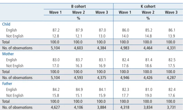
Table 2.12 shows the percentage of children, mothers and fathers who spoke English and non-English languages at each of the first three waves of the study. Children were less likely than their parents to mainly speak a language other than English at home.
Table 2.12 Main language spoken at home (English or non-English), by study child, their mother and their father, B and K cohorts, Waves 1–3
B cohort K cohort
Wave 1 Wave 2 Wave 3 Wave 1 Wave 2 Wave 3
% % Child English 87.2 87.9 87.0 86.0 85.2 86.1 Not English 12.8 12.1 13.0 14.0 14.8 13.9 Total 100.0 100.0 100.0 100.0 100.0 100.0 No. of observations 5,104 4,603 4,384 4,983 4,464 4,331 Mother English 83.0 83.7 83.1 82.4 81.4 82.5 Not English 17.0 16.3 16.9 17.6 18.6 17.5 Total 100.0 100.0 100.0 100.0 100.0 100.0 No. of observations 5,104 4,593 4,375 4,946 4,426 4,287 Father English 84.2 84.9 84.1 82.3 81.0 82.4 Not English 15.8 15.1 15.9 17.7 19.0 17.6 Total 100.0 100.0 100.0 100.0 100.0 100.0 No. of observations 4,627 4,106 3,884 4,318 3,834 3,731
Identification as Aboriginal and Torres Strait Islander
Study participants were asked whether the study child and/or their parent(s) identified as Aboriginal or Torres Strait Islander. There were 5,107 child observations, 5,104 mother observations and 4,627 father observations in the B cohort. There were 4,981 child observations, 4,944 mother observations and 4,316 father observations in the K cohort. Figure 2.7 shows that B cohort families were slightly more likely to identify as Indigenous. For the B and K cohort respectively, 5% and 4% of children identified as Indigenous, and 4% and 3% of mothers did so, as did 2% of fathers in both cohorts.
4.9 3.5 2.2 3.9 2.8 1.9 0 1 2 3 4 5 6
Child Mother Father
Percentage identified as Indigenous
B cohort K cohort
Figure 2.7 Distribution of children, mothers and fathers who identified as Aboriginal or Torres Strait Islander, B and K cohorts, Wave 1
Families who identified as Aboriginal or Torres Strait Islanders were not used as a comparison subpopulation throughout the report due to the small size of this subpopulation, and because of concerns about the representativeness of the group (Hunter, 2008).
2.5 Further reading
Gray, M., & Sanson, A. (2005). Growing Up in Australia: The Longitudinal Study of Australian Children. Family Matters, 72, 4–9.
Qu, L., Soriano, G., & Weston, R. (2006). Starting early, starting late: Socio-demographic characteristics and parenting of new mothers of different ages. Family Matters, 73, 52–59.
Sanson, A., Johnstone, R., LSAC Research Consortium, & FaCS LSAC Project Team. (2004). Growing Up in Australia takes its first steps. Family Matters, 67, 46–52.
Soloff, C., Lawrence, D., & Johnstone, D. (2005) LSAC sample design (Technical Paper No. 1). Melbourne: Australian Institute of Family Studies.
2.6 References
Australian Bureau of Statistics. (2005). Australian Standard Classification of Languages (ASCL) 2005–06 (Cat. No. 1267.0). Canberra: ABS.
Australian Bureau of Statistics. (2008). Standard Australian Classification of Countries (SACC) (2nd Ed.) (Cat No. 1269.0). Canberra: ABS.
Blakemore, T., Strazdins, L., & Gibbings, J. (2009). Measuring family socioeconomic position. Australian Social Policy, 8, 121–168.
Hunter, B. (2008). Benchmarking the Indigenous sub-sample of the Longitudinal Study of Australian Children. Australian Social Policy, 7, 61–84.
Soloff, C., Lawrence, D., Misson, S., & Johnstone, R. (2006). Wave 1 weighting and non-response (Technical Paper No. 3). Melbourne: Australian Institute of Family Studies.
Chapter 3: How family composition changes across waves
3
Brigit Maguire
Australian Institute of Family Studies
How family composition
changes across waves
C
hildren grow up in many different kinds of families, and children’s family environments often change as they move through childhood. These family environments and the changes children experience can greatly influence their development and outcomes (de Vaus & Gray, 2003; Pryor & Rodgers, 2001). Growing Up in Australia: The Longitudinal Study of Australian Children (LSAC) provides an opportunity to examine changing family composition and characteristics over time.This chapter presents analyses using the first three waves of the study to explore changes in family characteristics, focusing on children’s parents and siblings.1 The first section looks at the
types of families in which children live (e.g., whether children live with one or both of their biological parents), the characteristics of lone parents, and parents’ relationship status. The second section focuses on children’s siblings, parents with other children living elsewhere, and children experiencing changes in the residents of their households.
Throughout this chapter, the terms “family” and “household” both refer to the child’s main household; that is, the household in which the child lives with their primary parent (Parent 1). The characteristics of children’s secondary households (i.e., with a parent living elsewhere after parental separation) will be examined in future reports. The relationships between parents and children reported throughout this chapter are derived using the study respondents’ description of the relationships between the study child, primary parent, secondary parent, and other household members. The different descriptions of children’s parents used throughout this chapter are explained in Box 3.1.
3.1 Children’s parents
Family type: With how many and which parents do children live?
The majority of Australian children live in one of three major family types: with two biological parents, with one biological parent only, or with a biological parent and a step-parent.2 This sectionexamines the percentages of children living in these three types of families,3 and how children’s
family structures change across the first three waves.
Table 3.1 shows the percentages of children in the three major family types at each wave. The majority of children in both cohorts lived with both biological parents at all three waves. However,
1 A small percentage of children lived with other people in addition to their parents or siblings, such as grandparents, other relatives, boarders or housemates. These percentages were similar for the B and K cohorts across the first three waves of the study, ranging from 8% to 10%.
2 Same-sex couple parents are not distinguished from other parents throughout this chapter. There were fewer than ten families with two mothers and no families with two fathers at each of the first three waves, so these families cannot be analysed separately. In most of these same-sex couple families, the child was described as having a biological mother and a step-mother or adoptive mother, and the parents’ relationship was classified as de facto. 3 While the majority of children lived in one of the three major family types, a small percentage (fewer than 1%) lived with different types of parents at each of the first three waves of the study. These children lived only with non-biological parents (e.g., foster parents, grandparents, other relatives), or with one biological parent and another non-biological parent who was n