Performance Analysis: Data,
Dependence and Extremes
Fei He
Submitted in partial fulfillment of the requirements for the degree
of Doctor of Philosophy
in the Graduate School of Arts and Sciences
COLUMBIA UNIVERSITY
Fei He All Rights Reserved
Distributionally Robust Performance Analysis:
Data, Dependence and Extremes
Fei He
This dissertation focuses on distributionally robust performance analysis, which is an area of applied probability whose aim is to quantify the impact of model errors. Stochas-tic models are built to describe phenomena of interest with the intent of gaining insights or making informed decisions. Typically, however, the fidelity of these models (i.e. how closely they describe the underlying reality) may be compromised due to either the lack of information available or tractability considerations. The goal of distributionally robust performance analysis is then to quantify, and potentially mitigate, the impact of errors or model misspecifications. As such, distributionally robust performance analysis affects virtually any area in which stochastic modelling is used for analysis or decision making.
This dissertation studies various aspects of distributionally robust performance analysis. For example, we are concerned with quantifying the impact of model error in tail estimation using extreme value theory. We are also concerned with the impact of the dependence structure in risk analysis when marginal distributions of risk factors are known. In addition, we also are interested in connections recently found to machine learning and other statistical estimators which are based on distributionally robust optimization.
The first problem that we consider consists in studying the impact of model specifica-tion in the context of extreme quantiles and tail probabilities. There is a rich statistical theory that allows to extrapolate tail behavior based on limited information. This body of theory is known as extreme value theory and it has been successfully applied to a wide range of settings, including building physical infrastructure to withstand extreme environ-mental events and also guiding the capital requirements of insurance companies to ensure their financial solvency. Not surprisingly, attempting to extrapolate out into the tail of a
of models (known as generalized extreme value distributions) can be used to perform tail estimation. Because such assumptions are so difficult (or impossible) to be verified, we use distributionally robust optimization to enhance extreme value statistical analysis. Our approach results in a procedure which can be easily applied in conjunction with standard extreme value analysis and we show that our estimators enjoy correct coverage even in settings in which the assumptions imposed by extreme value theory fail to hold.
In addition to extreme value estimation, which is associated to risk analysis via extreme events, another feature which often plays a role in the risk analysis is the impact of de-pendence structure among risk factors. In the second chapter we study the question of evaluating the worst-case expected cost involving two sources of uncertainty, each of them with a specific marginal probability distribution. The worst-case expectation is optimized over all joint probability distributions which are consistent with the marginal distributions specified for each source of uncertainty. So, our formulation allows to capture the impact of the dependence structure of the risk factors. This formulation is equivalent to the so-called Monge-Kantorovich problem studied in optimal transport theory, whose theoretical prop-erties have been studied in the literature substantially. However, rates of convergence of computational algorithms for this problem have been studied only recently. We show that if one of the random variables takes finitely many values, a direct Monte Carlo approach al-lows to evaluate such worst case expectation withO(n−1/2) convergence rate as the number of Monte Carlo samples, n, increases to infinity.
Next, we continue our investigation of worst-case expectations in the context of multiple risk factors, not only two of them, assuming that their marginal probability distributions are fixed. This problem does not fit the mold of standard optimal transport (or Monge-Kantorovich) problems. We consider, however, cost functions which are separable in the sense of being a sum of functions which depend on adjacent pairs of risk factors (think of the factors indexed by time). In this setting, we are able to reduce the problem to the study of several separate Monge-Kantorovich problems. Moreover, we explain how we can even include martingale constraints which are often natural to consider in settings such as
in the later parts of the dissertation we take a broader view by studying decisions which are made based on empirical observations. So, we focus on so-called distributionally robust optimization formulations. We use optimal transport theory to model the degree of distri-butional uncertainty or model misspecification. Distridistri-butionally robust optimization based on optimal transport has been a very active research topic in recent years, our contribution consists in studying how to specify the optimal transport metric in a data-driven way. We explain our procedure in the context of classification, which is of substantial importance in machine learning applications.
List of Figures iv
List of Tables v
1 Introduction 1
2 On Distributionally Robust Extreme Value Analysis 11
2.1 Introduction . . . 11
2.1.1 Motivation and Standard Approach . . . 12
2.1.2 Proposed Approach Based on Infinite Dimensional Optimization . . 13
2.1.3 Choosing Discrepancy and Consistency Results . . . 14
2.1.4 The Final Estimation Procedure . . . 16
2.2 Generalized extreme value distributions . . . 16
2.2.1 Frechet, Gumbel and Weibull types . . . 17
2.2.2 On model errors and robustness . . . 19
2.3 A non-parametric framework for addressing model errors . . . 20
2.3.1 Divergence measures . . . 20
2.3.2 Robust bounds via maximization of convex integral functionals . . . 21
2.4 Asymptotic analysis of robust estimates of tail probabilities . . . 24
2.5 Robust estimation of VaR . . . 27
2.5.1 On specifying the parameterδ. . . 30
2.5.2 On specifying the parameterα. . . 31
2.5.3 Numerical examples . . . 34
3 Dependence with two sources of uncertainty: Computing Worst-case
Ex-pectations Given Marginals via Simulation 46
3.1 Algorithmic Description . . . 49
3.2 Convergence Analysis . . . 49
3.2.1 Proof of Theorem 3.1 . . . 50
3.3 Additional Discussion and Extensions . . . 55
4 Dependence with several sources of uncertainty: Martingale Optimal Transport with the Markov Property 57 4.1 Introduction . . . 57
4.2 Optimal Transport Problems with Two Marginal Distributions and Minimum Cost Problems . . . 59
4.2.1 Problem Definition . . . 59
4.2.2 Quantization and Discretization . . . 60
4.3 Optimal Transport Problems with d-Marginals . . . 61
4.3.1 Discretization and Complexity . . . 62
4.4 Martingale Optimal Transport Problems with Separable Cost Functions and the Markov Property . . . 63
4.4.1 Applications in Pricing Exotic Options . . . 66
4.5 A Numerical Experiment . . . 68
5 Data-driven choice of the aspects over which to robustify: Data-driven Optimal Transport Cost Selection and Doubly Robust Distributionally Robust Optimization 70 5.1 Introduction . . . 70
5.2 Data-Driven DRO: Intuition and Interpretations . . . 75
5.3 Background on Optimal Transport and Metric Learning Procedures . . . . 77
5.3.1 Defining Optimal Transport Distances and Discrepancies . . . 77
5.3.2 On Metric Learning Procedures . . . 78
5.6 Robust Metric Learning . . . 86
5.6.1 Robust Optimization for Relative Metric Learning . . . 86
5.6.2 Robust Optimization for Absolute Metric Learning . . . 88
5.7 Numerical Experiments . . . 91
5.7.1 Numerical Experiments for DD-DRO . . . 91
5.7.2 Numerical Experiments for DD-R-DRO . . . 92
5.8 Conclusion and Discussion . . . 93
5.9 Proof of Main Results . . . 94
5.9.1 Proof of Theorem 5.1 . . . 94
5.9.2 Proof of Lemma 5.1 . . . 97
Bibliography 98
2.1 Comparison of ¯Fα,δ(x) for different GEV models: The solid curves represents the reference modelGγref(x) forγref = 1/3 (top left figure),γref = 0 (top right
figure) and γref = −1/3 (bottom figure). Computations of corresponding ¯
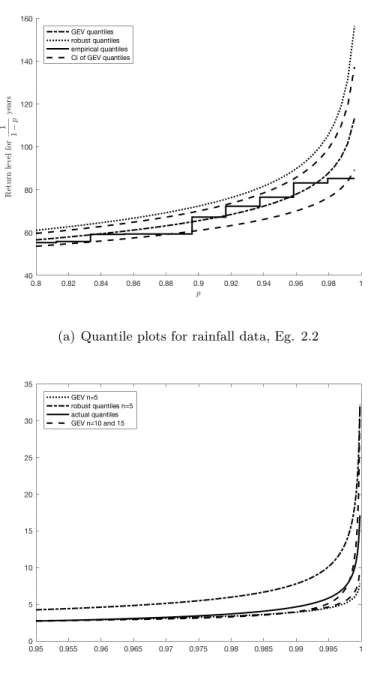
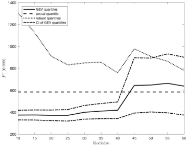
Fα,δ(x) are done for α = 1 (the dotted curves), and α = 5 (the dash-dot curves) with δ fixed at 0.1. The dotted curves (corresponding to α = 1, the KL-divergence case) conform with our reasoning that ¯Fα,δ(x) have vastly different tail behaviours from the reference models when KL-divergence is used. 29 2.2 Plots for Examples 2.2 and 2.3 . . . 35 2.3 Plot for Example 2.4, instability in estimated quantile F←(0.999) . . . 37 5.1 Four diagrams illustrating information on robustness. . . 75 5.2 Stylized examples illustrating the need for data-driven cost function. . . . 76
2.1 A summary of domains of attraction ofFα,δ(x) = 1−F¯α,δ(x) for GEV models. Throughout the paper, γ∗ := αα−1γref
. . . 28
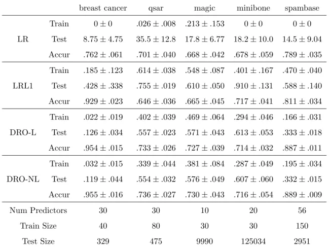
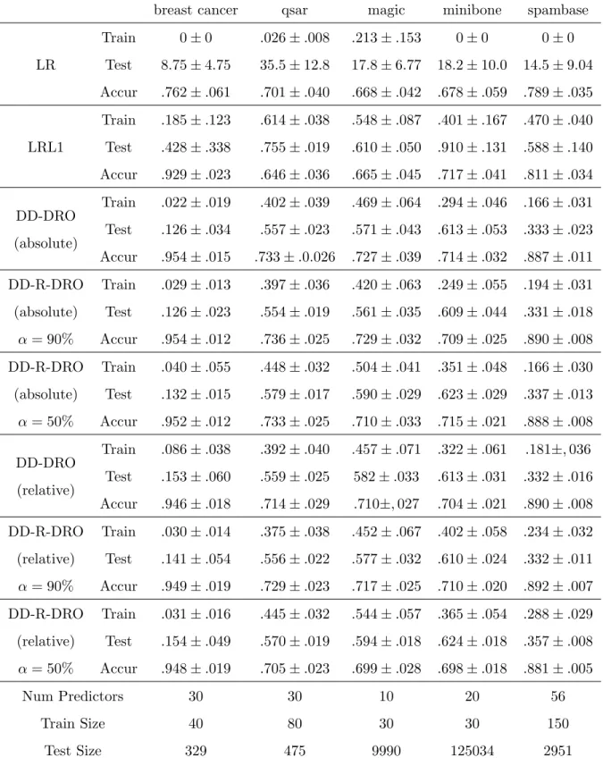
5.1 Numerical Results for DD-DRO on Real Data Sets. . . 92 5.2 Numerical Results for DD-R-DRO on Real Data Sets with Side Information
Generated byk-NN Method. . . 99
First and foremost, I would like to thank my advisor, Professor Jose Blanchet, for his continued generous support. His broad knowledge, great insight and unwavering dedication to research have always encouraged and inspired me to pursue interesting research topics and helped me overcome many challenges and difficulties.
Besides my advisor, I would like to thank the rest of my committee members: Prof. David Yao, Prof. Karl Sigman, Prof. Henry Lam and Prof. Jing Dong, for offering their invaluable insight and expertise to improve my dissertation. I have learned much from Prof. Yao and Prof. Sigman’s probability courses. Henry and Jing are also my research collaborators and I really appreciate their guidance and patience during the collaboration. I am also grateful to many IEOR professors, especially Prof. Garud Iyengar, Prof. Martin Haugh, Prof. Agostino Capponi, Prof. Jay Sethuraman, Prof. Tim Leung and Prof. Marcel Nutz, as well as many doctoral students and friends, especially Zhipeng Liu, Yanan Pei, Anran Li, Yang Kang, Kartheyek Murthy, Ni Ma, Xinshang Wang, Mingxian Zhong, Chaoxu Zhou, Francois Fagan, Octavio Ruiz Lacedelli, Di Xiao, Kevin Guo, Brian Ward, Bin Qi, Yang Zhang, Yangbin Li, Xin Li, Zheng Wang, Jianshu Wu, Linan Yang, Juan Li, Yin Lu, Yunhao Tang, Fan Zhang, Fengpei Li and Raghav Singal.
I would also like to thank Prof. Mark Podolskij, Prof. Rainer Dahlhaus, Prof. Tilmann Gneiting, Yu Hao, Stefan Richter, Brandon Williams, Yuhong Dai, Nopporn Thamrongrat, Cike Peng, Julie Yuan Merten, Shuxin Chen and Claudio Heinrich for their support and help during my study in Germany. I am also much obliged to many friends in China: Chengbin Peng, Hao Zhang, Junhui Zhang, Lu Chen, Huajie Mao, Hongyu Zhu, Wei Lin, Minjie Zhang, Fang Lv, Hongyu Zhu, Bo Zhang, Wei Shi, Xiyuan Chen, Dingsheng Lin and Yu Shi.
Last but not least, I am deeply indebted to my parents and Chris for their unconditional
Chapter 1
Introduction
This dissertation focuses on distributionally robust performance analysis, which is an area of applied probability whose aim is to quantify the impact of model errors. Stochastic models are built to describe phenomena of interest with the intent of gaining insights or making informed decisions. Typically, however, the fidelity of these models (i.e. how closely they describe the underlying reality) may be compromised by either the lack of information available or by tractability considerations. The goal of distributionally robust performance analysis is then to quantify, and potentially mitigate, the impact of errors or model mis-specifications. As such, distributionally robust performance analysis affects virtually any area in which stochastic modelling is used for analysis or decision making.
More specifically, in a stochastic model, the performance evaluation can be represented asEP[h(X)] for a given probability measure P, a random variable X and a function h. A modeler faces the task of choosing a probability model P which is not only close to the reality but is also tractable. However, this procedure will often suffer from model errors, either due to the lack of data or due to the estimation errors.
A popular approach to address this problem is by considering the distributionally robust bound as the optimal value of the optimization problem
sup P∈UEP
[h(X)],
over a family of plausible alternative probability models U. A natural way to specify the familyU is by defining an uncertainty neighborhood{P :d(P, Pref)≤δ}, wherePref is the
chosen reference model and δ is a tolerance level. Here d is a metric which measures the discrepancy between two probability measures. Popular choices fordare the KL-divergence (Breuer and Csiszar (2013a), H.Lam (2013), Glasserman and Xu (2014a)) and the Wasser-stein distances (Esfahani and Kuhn (2015), Wozabal (2012), Blanchet and Murthy (2016)) to quantify the model uncertainty. Despite the fact that KL-divergence is not a true metric, KL-divergence is a popular choice due to its tractability. This approach provides a bound for the performance evaluation regardless of the probability measure used as long as such measures stay within a prescribed toleranceδ of an appropriate reference model.
In Chapter 2 we study the distributional robustness in the context of the extreme value theory (EVT). Our focus is closer in spirit to distributionally robust optimizations as in, for instance, Dupuiset al. (2000), Hansen and Sargent (2001), Ben-Talet al. (2013), Breuer and Csisz´ar (2013b). However, in contrast to the literature on robust optimization, the emphasis here is on understanding the implications of distributional uncertainty regions in the context of EVT. As far as we know this is the first paper that studies distributional robustness in the context of EVT. Here, our objective is to provide a robust bound for the estimate of the value at risk of a risk factor X,
VaRp(X) =F←(p) := inf{x:P{X≤x} ≥p}, forp∈(0,1).
EVT provides reasonable statistical principles which can be used to extrapolate tail distri-butions and then estimate this extreme quantiles. In particular, we focus on the classical block maxima approach for the extrapolation, that is, we divide the i.i.d. data Xi into several blocks, where each block containsn data points. Then we pick the maximum value Mn from each block. The Fisher-Tippett-Gnedenko theorem ensures that under certain assumptions of the underlying distribution of the Xi, the maximum Mn has some types of limiting distribution PGEV, the so-called generalized extreme value distribution, and produces PGEV−1 (pn) as an estimate for the quantile VaR
p(X). However, as with any form for extrapolation, extreme value analysis rests on assumptions that are rather difficult (or impossible) to verify. Therefore, it makes sense to provide a mechanism to robustify the inference obtained via EVT. Similarly we formulate the robust estimate through an un-certainty neighborhood of the limiting distribution with radius δ and then give a robust
estimate of VaRp(X) by
sup{G←(pn) :d(G, PGEV)≤δ}.
Here, we choose d as the R´enyi divergence, also called the α-divergence, which includes KL-divergence as a special case forα = 1. We show that using KL-divergence to form the uncertainty set around PGEV would include a probability measure whose tail probabilities decay at an unrealistically slow rate and the parameter α gives modeler the freedom to tune the uncertainty set and include distributions with tails are heavier than the reference model but not prohibitively heavy. We give concrete algorithms to calculate this robust estimate and we also provide some practical ways to specify the hyperparametersαand the radius of the uncertainty set δ. We also give some examples where the standard EVT can significantly underestimate the quantiles of interest while our estimator is quite robust and at the same time not too conservative.
In addition to extreme value estimation, which is associated to risk analysis via extreme events, another feature which often plays a role in the risk analysis is the impact of de-pendence structure among risk factors. Chapter 3 and Chapter 4 are devoted to find the lower or upper bounds among any dependence structure with two sources of uncertainty or multiple sources of uncertainty, that is, measuring the impact of the joint distribution with two or multiple fixed marginals.
In Chapter 3 we study a direct Monte-Carlo-based approach for computing lower and upper bounds among any dependence structure for a function of two random vectors whose marginal distributions are assumed to be known.
More precisely, suppose that X ∈ Rd follows distribution µ and Y ∈
Rl follows dis-tribution ν. We define Π (µ, ν) to be the set of joint distributions π in Rd×l such that the marginal of the first d entries coincides with µ and the marginal of the last l entries coincides withν. In other words, for any probability measure π inRd×l (endowed with the Borel σ-field), if we let πX(A) = π A×Rl for any Borel measurable set A ∈ Rd, and πY (B) =π Rd×B for any Borel measurable setB ∈Rl, then π∈Π (µ, ν) if and only if πX =µ andπY =ν. We are interested in the quantity (focusing on minimization)
wherec(·,·)∈Ris some cost function. Formulation (1.1) is well-defined as the class Π (µ, ν) is non-empty, because the product measure π =µ×ν belongs to Π (µ, ν). The worst-case expectation is optimized over all joint probability distributions which are consistent with the marginal distributions specified for each source of uncertainty. So, our formulation allows to capture the impact of the dependence structure of the risk factors. This formulation is equivalent to the so-called Monge-Kantorovich problem studied in optimal transport theory, whose theoretical properties have been studied in the literature substantially (Villani (2003), Villani (2008)).
We focus on the setting where one of the marginals, say Y, has a distribution ν with finite support{y1, ..., ym} ⊂Rl and another, sayX, has a multi-dimensional distributionµ that can be continuous. Suppose we can i.i.d. sampleXi, i= 1, . . . , nfrom the distribution µthen we approximate V by
Vn= min{Eπ[c(X, Y)] :π ∈Π (µn, ν)} (1.2) whereµn is the empirical distribution of X constructed from theXi’s, i.e.,
µn(A) = 1 n n X i=1 I(Xi ∈A) for any Borel measurableA.
Our main result shows that the error of our procedure isO(n−1/2) wherenis the sample size, independent of the dimension dorl. We also identify the limiting distribution in the associated CLT. The closest work to our results, as far as we know, is the recent work of Sommerfeld and Munk (2016), which derives a CLT when both marginal distributions are finitely discrete.
On the other hand, it is difficult to further generalize our procedure to the case when bothXandY are continuous. The study on the rate of convergence in Wasserstein distance of the empirical measure gives ideas that in this general case the convergence rate fail to retainO(n−1/2) (Fournier and Guillin (2015)). For instance, suppose bothX, Y ∼U[0,1]d, i.e. µ = ν are d-dim uniform distributions, and c(x, y) = kx−yk, the optimal value V corresponds to the Wasserstein distance (of order 1) between X and Y, which is of course 0. It is well-known that sampling X and keeping Y continuous will give, for d ≥ 3, an
expected optimal value of Vn= min{Eπ[c(X, Y)] :π∈Π (µn, µ)} µn(·) := 1 n n X i=1 I(Xi ∈ ·)
is of ordern−1/d, i.e.,C1n−1/d≤EVn≤C2n−1/d for all nfor some C1, C2 >0 (see e.g.van
Handel (2014)).
In Chapter 4 we study a discretization approach for computing lower and upper bounds among any dependence structure for a function of multiple random vectors whose marginal distributions are assumed to be known. Givendmarginal distributionsµ1, . . . , µd on a common compact metric spaceX, we focus on the lower bound
inf π∈Π(µ1,...,µd)
Eπ[c(X1, . . . , Xd)], (1.3) where Π(µ1, . . . , µd) is the set of all joint distributions with marginalsX1 ∼µ1, . . . , Xd∼µd, and c is a cost function. Note that when d= 2, the problem (1.3) is the standard optimal transport problem. Ford >2, this problem has been studied by Gangbo and Swiech (1998) and G.Carlier et al. (2008). Such problems often arise from risk management, where the performance depends ondrisk factors, and the marginal distributions of each risk factor is known but the dependence structure is ambiguous.
We approach this problem by first create a partition of the compact spaceX withX = Pn
k=1Ak such that the diameter of everyAk does not exceedδ, withδ =O(n−1). Then we choose a representativexk∈Ak for eachkand form a discrete setXδ={xk :k= 1, . . . , n} with an associated quantization map
T :X →Xδ x7→ n X k=1 xkI(x∈Ak). In addition, we define the corresponding quantized measures as
Then the discretized approximate version of the problem is as follows: min π n X i1,···,id=1 c(xi1,· · · , xid)π(xi1,· · · , xid) s.t. n X i2=1,···,id=1 π(xi1,· · · , xid) =µ1,δ(xi1), i1 = 1,· · ·, n, · · · n X i1=1,···,id−1=1 π(xi1,· · ·, xid) =µd,δ(xid), id= 1,· · · , n, n X i1=1,···,id=1 π(xi1,· · ·, xid) = 1, π(xi1,· · ·, xid)≥0,
Ford= 2, it is an assignment problem, which can be solved by various network algorithms that are much faster than the general LP algorithms. For instance, with the successive shortest path algorithm (see R.K.Ahuja et al. (2000) p.320) one can achieveO(n2log(n)). We will also quantify the error bounds for the difference between the true optimal value and the optimal value of the discretized version. Ford >2 we can in general not transform it to assignment problems except when the cost function cis separable, that is,ctakes the form of c(X1,· · ·, Xd) =
Pd−1
k=1ct(Xt, Xt+1), where ct, t = 1,· · ·, d−1 are cost functions depending only on the two adjacent marginals Xt and Xt+1. Then the above discretized
version can be decomposed intod−1 assignment problems and hence can be solved efficiently by using network algorithms. In fact, with this separable cost function, we can apply this discretization approach to the so-called martingale optimal transport problem, which is first studied by Beiglbock et al. (2013) and Galichon et al. (2014). A general form of the martingale optimal transport problem looks as follows:
inf π∈M(µ1,...,µd)
Eπ[c(X1, . . . , Xd)], (1.5) where M(µ1, . . . , µd) is the set of all martingale measures, i.e. the underlying process (Xt)t=1,...,d satisfiesXt∼µt,Eπ[Xt|Ft−1] =Xt−1. The martingale optimal transport
prob-lem is different from the previous one in that in general there exists no easy way to convert it to the discretized version due to the martingale constraint, but we can show that when
the cost function c is separable, then the problem can still be discretized to d−1 linear programming problems.
A major application of martingale optimal transport problem is in mathematical finance, where it is important to choose a pricing model when evaluating an exotic option; such a model is characterized by a martingale measure while the marginal distributions are the daily underlying prices. Instead of postulating a model, we use (1.5) to give a model-free lower bound for the price of exotics, whose payoff function c depends on the d-marginal distributions of a certain underlying X, indexed by time t= 1,· · ·, d. Similarly, by maxi-mization instead of minimaxi-mization we also obtain an upper bound for the price. This price range is robust against model errors and it complies with market prices of vanilla options, which are liquid and suitable hedging instruments. We provide some examples of financial derivatives whose model-free price ranges can be obtained by our method.
While in the previous chapters we focused on the impact of tail modeling or dependence, in the later parts of the dissertation we take a broader view by studying decisions which are made based on empirical observations. We focus on so-called distributionally robust opti-mization formulations. The objective of distributionally robust optiopti-mization is to choose a decision β that minimizes the worst-case expected loss supP∈UEP[l(X, β)], where the worst-case is taken over an uncertainty neighborhood U of an unknown true distribution P∗. Though the true distribution P∗ is unknown, we usually have some information or properties about P∗, such as the empirical measure Pn, so in practice we often form the uncertainty neighborhood around Pn. Distributionally robust optimization has two main advantages: one is to improve the out-of-sample performance of stochastic programmings and the other one is that distributionally robust models are often tractable even though the corresponding stochastic models are NP-hard. A good choice of uncertainty neighborhood U should be rich enough to include the true distribution with high confidence while at the same time it should be small enough to exclude uninteresting distributions so as to avoid too conservative decisions. Previous works usually use moment constraints (J.Goh and M.Sim (2010), Wieseman et al. (2014)) and KL-divergence (Breuer and Csiszar (2013a), H.Lam (2013), Glasserman and Xu (2014a)) to quantify model misspecification and model
uncer-tainty. Despite the fact that KL-divergence is not a true metric, it is a popular choice due to its tractability. However, many of these earlier works also acknowledge the shortcom-ings of KL-divergence, as the absolute continuity requirement rules out many interesting settings. For instance, all the probability measures in the neighborhood of an empirical measure defined by the KL-divergence are just re-weighting of this empirical measure; the neighborhood fails to include any continuous measures. Recently, people start applying Wasserstein distance to distributionally robust optimization and quantify model misspeci-fication (Wozabal (2012), Esfahani and Kuhn (2015), Blanchet and Murthy (2016)). When the cost function c is a metric, i.e. c(x, y) = d(x, y), then the optimal transport problem actually induces a metric called the Wasserstein distance or the optimal transport metric, which characterizes a distance between the two probability measures µand ν, and in turn we can use it to define a neighborhood of a measure and apply it to the distributionally robust problems. The uncertainty set contains both continuous and discrete distributions that are close to the measure of interest (e.g. the empirical measure) with respect to the Wasserstein distance, which makes it possible to incorporate many tractable surrogate mod-els and offers better out-of-sample performance. However, distributionally robust modmod-els with Wasserstein uncertainty neighborhood are generally harder in computations and they are still attractive topics in research.
Chapter 5 uses optimal transport theory to model the degree of distributional uncer-tainty or model misspecification, and extends the following distributionally robust optimiza-tion (DRO) model proposed by Blanchet et al. (2016a), where they reveal that the DRO models links to several machine learning algorithms such as regularized logistic regression for classification, min β P∈Umaxδ(Pn) EP[l(X, Y, β)] = min β EPn[l(X, Y, β)] +δkβkp , (1.6)
where l is some loss function, andUδ(Pn) ={P :Dc(P, Pn)≤δ} is a neighborhood of the empirical measure Pn defined by the optimal transport distance
Dc(P, Pn) = inf π
Eπ[c(P, Pn)] :π is a joint distribution ofP and Pn} and the optimal transport cost function
c((x, y),(x0, y0)) =x−x0 2 qI(y=y 0 ) +∞ ·I(y6=y0),
where p−1 +q−1 = 1 for p ∈ [1,∞), and EPn[l(X, Y, β)] :=
1
n Pn
i=1l(Xi, Yi, β). We can
interpret the DRO problem on the left hand side of (1.6) as we choose a decision β for minimization, while the adversarial player selects a modelP, a perturbation of the dataPn, fromUδ(Pn). This interpretation has applications in adversarial training of neural networks, see e.g. Sinhaet al.(2017). Note that theshapeofUδ(Pn) is determined by the cost function c(·) in the definition of the optimal transport discrepancyDc(P, Pn), but so far it has been taken as a given`q-norm, but not chosen in a data-driven way; this is the starting point of this project to improve the DRO method.
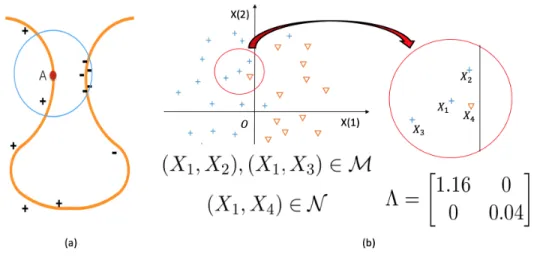
Our contribution consists in studying how to specify the optimal transport metric in a data-driven way. We would propose a data-driven DRO (DD-DRO) model with the cost functioncΛdefined by a local metricdΛ(x, x0) :=
p
(x−x0)TΛ(x)(x−x0), where the matrix
Λ(x) is trained by metric learning methods, see, e.g. Belletet al.(2013). Note that when we use a data-driven cost function, we may no longer have correspondence as (1.6) but we can still directly solve the DRO problem on the left hand side. We expect that DD-DRO is able to improve the generalization property compared to many other state-of-the-art classifiers on a large number of data sets from UCI machine learning database, because it exploits the side information (the information about the intrinsic metric, the “shape”) of the data.
The main methodologies and contributions of this project are the followings:
• We would use DRO as a link that combines k-NN methods with logistic regressions for classification. We use k-NN method to generate the side information of the data and then form the shape of the distributional uncertainty neighborhood by learning a metric from this side information.
• The DD-DRO is able to recover adaptive regularized ridge regression estimator. The DD-DRO provides a novel and interpretable way to select hyper-parameters in adap-tive regularized ridge regression (see e.g.Zou (2006)) from a metric learning perspec-tive.
• We would use an approximation algorithm based on stochastic gradient descent to solve DD-DRO. We would reformulate the DRO problem by using the duality repre-sentation given in Blanchet and Murthy (2016) and then solve it by smooth
approxi-mation and stochastic gradient descend algorithms.
• We would employ the robust metric learning to deal with the noisiness of side infor-mation. Since the side information is usually noisy, we borrow the idea from robust optimization (see e.g. Ben-Talet al.(2009)) and build a doubly robust data-driven dis-tributionally robust optimization (DD-R-DRO) model on top of the DD-DRO model to achieve robust metric learning.
Chapter 2
On Distributionally Robust
Extreme Value Analysis
2.1
Introduction
Extreme Value Theory (EVT) provides reasonable statistical principles which can be used to extrapolate tail distributions, and, consequently, estimate extreme quantiles. However, as with any form for extrapolation, extreme value analysis rests on assumptions that are rather difficult (or impossible) to verify. Therefore, it makes sense to provide a mechanism to robustify the inference obtained via EVT.
The goal of this paper is to study non-parametric distributional robustness (i.e. find-ing the worst case distribution within some discrepancy of a natural baseline model) in the context of EVT. We ultimately provide a data-driven method for estimating extreme quantiles in a manner that is robust against possibly incorrect model assumptions. Our objective here is different from standard statistical robustness which is concerned with data contamination only (not model error); see, for example, Tsaiet al. (2010), for this type of analysis in the setting of EVT.
Our focus in this paper is closer in spirit to distributionally robust optimization as in, for instance, Dupuiset al.(2000), Hansen and Sargent (2001), Ben-Talet al.(2013), Breuer and Csisz´ar (2013b). However, in contrast to the literature on robust optimization, the emphasis here is on understanding the implications of distributional uncertainty regions in
the context of EVT. As far as we know this is the first paper that studies distributional robustness in the context of EVT.
We now describe the content of the paper, following the logic which motivates the use of EVT.
2.1.1 Motivation and Standard Approach
In order to provide a more detailed description of the content of this paper, its motivations, the specific contributions, and the methods involved, let us invoke a couple of typical ex-amples which motivate the use of extreme value theory. As a first example, consider the problem of forecasting the necessary strength that is required for a skyscraper in New York City to withstand a wind speed that gets exceeded only about once in 1000 years, using wind speed data that is observed only over the last 200 years. In another instance, given the losses observed during the last few decades, a reinsurance firm may want to compute, as required by Solvency II standard, a capital requirement that is needed to withstand all but about one loss in 200 years.
These tasks, and many others in practice, present a common challenge of extrapolating tail distributions over regions involving unobserved evidence from available observations. There are many reasonable ways of doing these types of extrapolations. One might take advantage of physical principles and additional information, if available, in the windspeed setting; or use economic principles in the reinsurance setting. In the absence of any funda-mental principles which inform tail extrapolation of a random variable X, one may opt to use purely statistical considerations.
One such statistical approach entails the application of the popular extremal types theorem (see Section 2.2) to model the distribution of block maxima of a modestly large number of samples of X, by a generalized extreme value (GEV) distribution. Once we have a satisfactory model for the distribution of Mn = max{X1, . . . , Xn}, evaluation of any desired quantile of X is straighforward because of the relationship that P(Mn≤x) = (P(X ≤ x))n for any x ∈ R. Another common approach is to use samples that exceed a certain threshold to model conditional distribution of X exceeding the threshold. The standard texts in extreme value theory (see, for example, Leadbetteret al. (1983),de Haan
and Ferreira (2006),Resnick (2008)) provide a comprehensive account of such standard statistical approaches.
Regardless of the technique used, various assumptions underlying an application of a result similar to the extremal types theorem might be subject to model error. Consequently, it has been widely accepted that tail risk measures, particularly for high confidence levels, can only be estimated with considerable statistical as well as model uncertainty (see, for example, Jorion (2006)). The following remark due to Coles (2001) holds significance in this discussion: “Though the GEV model is supported by mathematical argument, its use in extrapolation is based on unverifiable assumptions, and measures of uncertainty on return levels should properly be regarded aslower boundsthat could be much greater if uncertainty due to model correctness were taken into account.”
Despite these difficulties, however, EVT is widely used (see, for example, de Haan and Ferreira (2006)) and regarded as a reasonable way of extrapolation to estimate extreme quantiles.
2.1.2 Proposed Approach Based on Infinite Dimensional Optimization
We share the point of view that EVT is a reasonable approach, so we propose a procedure that builds on the use of EVT to provide upper bounds which attempts to address the types of errors discussed in the remark above from Coles (2001). For large values of n, under the assumptions of EVT, the distribution of Mn lies close to, and appears like, a GEV distribution. Therefore, instead of considering only the GEV distribution as a candidate model, we propose a non-parametric approach. In particular, we consider a family of probability models, all of which lie in a “neighborhood” of a GEV model, and compute a conservative worst-case estimate of Value at risk (VaR) over all of these candidate models. For p∈[0,1],the value at risk VaRp(X) is defined as
VaRp(X) =F←(p) := inf{x:P{X ≤x} ≥p}.
Mathematically, given a reference model, Pref, which we consider to be obtained using EVT (using a procedure such as the one outlined in the previous subsection), we consider
the optimization problem sup P{X > x}: d(P, Pref)≤δ . (2.1)
Note that the previous problem proposes optimizing over all probability measures that are within a tolerance level δ (in terms of a suitable discrepancy measure d) from the chosen baseline reference modelPref.
There is a wealth of literature that pursues this line of thought (see Dupuiset al.(2000), Hansen and Sargent (2001), Ahmadi-Javid (2012), Ben-Talet al.(2013),Breuer and Csisz´ar (2013b),Glasserman and Xu (2014b)), but, no study has been carried out in the context of EVT. Moreover, while the solvability of problems as in (2.1) have understandably received a great deal of attention, the qualitative differences that arise by using various choices of discrepancy measures,d, has not been explored, and this is an important contribution of this paper. For tractability reasons, the usual choice for discrepancydin the literature has been KL-divergence. In Section 2.3 we study the solution to infinite dimensional optimization problems such as (2.1) for a large class of discrepancies that includes KL-divergence as a special case, and discuss how such problems can be solved at no significant computational cost.
2.1.3 Choosing Discrepancy and Consistency Results
One of our main contributions in this paper is to systematically demonstrate the qualitative differences that arise by using different choices of discrepancy measures d in (2.1). Since our interest in the paper is limited to robust tail modeling via EVT, this narrow scope, in turn, lets us analyse the qualitative differences that may arise because of different choices of d.
As mentioned earlier, the KL-divergence1 is the most popular choice for d. In Section 2.4 we show that for any divergence neighborhood P, defined using d = KL-divergence around a baseline reference Pref, there exists a probability measure P in P that has tails
as heavy as
P(x,∞)≥clog−2Pref(x,∞),
for a suitable constantc, and all large enoughx.This means, irrespective of how smallδ is (smaller δ corresponds to smaller neighborhood P), a KL-divergence neighborhood around a commonly used distribution (such as exponential, (or) Weibull (or) Pareto) typically contains tail distributions that have infinite mean or variance, and whose tail probabilities decay at an unrealistically slow rate (even logarithmically slow, like log−2x, in the case of reference models that behave like a power-law or Pareto distribution). As a result, computations such as worst-case expected short-fall2 may turn out to be infinite. Such worst-case analyses are neither useful nor interesting.
For our purposes, we also consider a general family of divergence measures Dα that includes KL-divergence as a special case (when α = 1). It turns out that for any α > 1, the divergence neighborhoods defined as in {P :Dα(P, Pref)≤δ} consists of tails that are
heavier thanPref, but not prohibitively heavy. More importantly, we prove a “consistency” result in the sense that if the baseline reference model belongs to the maximum domain of attraction of a GEV distribution with shape parameter γref, then the corresponding worst-case tail distribution,
¯
Fα(x) := sup{P(x,∞) :Dα(P, Pref)≤δ}, (2.2)
belongs to the maximum domain of attraction of a GEV distribution with shape parameter γ∗ = (1−α−1)−1γref (if it exists).
Since our robustification approach is built resting on EVT principles, we see this consis-tency result as desirable. If a modeler who is familiar with certain type of data expects the EVT inference to result in an estimated shape parameter which is positive, then the robus-tification procedure should preserve this qualitative property. An analysis of the maximum domain of attraction of the distribution ¯Fα(x), depending on α and γref, is presented in
Section 2.4, along with a summary of the results in Table 1.
Note that the smaller the value ofα, the larger the absolute value of shape parameterγ∗, and consecutively, heavier the corresponding worst-case tail is. This indicates a gradation in the rate of decay of worst-case tail probabilities as parameter α decreases to 1, with
2
Similar to VaR, expected shortfall (or) conditional value at risk (referred as CVaR) is another widely recognized risk measure.
the case α = 1 (corresponding to KL-divergence) representing the extreme heavy-tailed behaviour. This gradation, as we shall see, offers a great deal of flexibility in modeling by letting us incorporate domain knowledge (or) expert opinions on the tail behaviour. If a modeler is suspicious about the EVT inference he/she could opt to selectα= 1, but, as we have mentioned earlier, this selection may result in pessimistic estimates.
The relevance of these results shall become more evident as we introduce the required terminology in the forthcoming sections. Meanwhile, Table 2.1 and Figure 2.1 offer illus-trative comparisons of ¯Fα(x) for various choices ofα.
2.1.4 The Final Estimation Procedure
The framework outlined in the previous subsections yields a data driven procedure for estimating VaR which is presented in Section 2.5. A summary of the overall procedure is given in Algorithm 2. The procedure is applied to various data sets, resulting in different reference models, and we emphasize the choice of different discrepancy measures via the parameter α. The numerical studies expose the salient points discussed in the previous subsections and rigorously studied via our theorems. For instance, Example 3 shows how the use of the KL divergence might lead to rather pessimistic estimates. Moreover, Example 4 illustrates how the direct application of EVT can severely underestimate the quantile of interest, while the procedure that we advocate provides correct coverage for the extreme quantile of interest.
The very last section of the paper, Section 2.6, contains technical proofs of various results invoked in the development.
2.2
Generalized extreme value distributions
The objective of this section is to mainly fix notation and review properties of generalized extreme value (GEV) distributions that are relevant for introducing and proving our main results in Section 2.4. For a thorough introduction to GEV distributions and their applica-tions to modeling extreme quantiles, we refer the readers to the wealth of literature that is available (see, for example, Leadbetter et al.(1983), Embrechts et al.(1997), de Haan and
Ferreira (2006), Resnick (2008) and references therein).
If we use Mn to denote the maxima of n independent copies of a random variable X with cumulative distribution funtion F(·),then extremal types theorem identifies all non-degenerate distributions G(·) that may occur in the limiting relationship,
lim n→∞P Mn−bn an ≤x = lim n→∞F n(a nx+bn) =G(x), (2.3) for every continuity pointxof G(·),withanand bnrepresenting suitable scaling constants. All such distributions G(x) that occur in the right-hand side of (2.3) are called extreme value distributions.
Extremal types theorem (Fisher and Tippet (1928), Gnedenko (1943)). The class of extreme value distributions is Gγ(ax+b) witha >0, b, γ∈R,and
Gγ(x) := exp
−(1 +γx)−1/γ
, 1 +γx >0. (2.4) Ifγ = 0,the right-hand side is interpreted as exp(−exp(−x)).
The extremal types theorem asserts that any G(x) that occurs in the right-hand side of (2.3) must be of the form Gγ(ax+b).As a convention, any probability distribution F(x) that gives rise to the limiting distribution G(x) =Gγ(ax+b) in (2.3) is said to belong to the maximum domain of attraction of Gγ(x). In short, it is written as F ∈ D(Gγ). The parametersγ, a >0 andbare, respectively, called the shape, scale and location parameters. From the above we have
P(Mn≤x) =P Mn−bn an ≤ x−bn an ≈Gγ0 x−bn an =:Gγ0(a0x+b0),
where γ0, an, bn are estimated by a parameter estimation technique such as maximum likelihood and a0 := 1/an, b0 := −bn/an. We will use PGEV to denote the distribution Gγ0(a0x+b0).
2.2.1 Frechet, Gumbel and Weibull types
Though the limiting distributionsGγ(ax+b) seem to constitute a simple parametric family, they include a wide-range of tail behaviours in their maximum domains of attraction, as
discussed below: For a distribution F,let ¯F(x) = 1−F(x) denote the corresponding tail probabilities, andx∗
F = sup{x:F(x)<1} denote the right endpoint of its support.
1) The Frechet Case (γ > 0).A distribution F ∈ D(Gγ) for some γ >0, if and only if right endpoint x∗F is unbounded, and its tail probabilities satisfy
¯
F(x) = L(x)
x1/γ, x >0 (2.5)
for a functionL(·) slowly varying at∞3. As a consequence, moments greater than or
equal to 1/γ do not exist. Any distribution F(x) that lies in D(Gγ) for some γ >0 is also said to belong to the maximum domain of attraction of a Frechet distribution with parameter 1/γ.The Pareto distribution 1−F(x) =x−α∧1 is an example for a distribution that belongs toD(G1/α).
2) The Weibull case (γ < 0).Unlike the Frechet case, a distribution F ∈ D(Gγ) for some γ < 0, if and only if its right endpoint x∗F is finite, and its tail probabilities satisfy ¯ F(x∗F −) =−1/γL 1 , >0 (2.6)
for a function L(·) slowly varying at ∞. A distribution that belongs to D(Gγ) for some γ < 0 is also said to belong to the maximum domain of attraction of Weibull family. The uniform distribution on the interval [0,1] is an example that belongs to this class of extreme value distributions.
3) The Gumbel case (γ = 0).A distribution F ∈ D(G0) if and only if
lim t↑x∗ F ¯ F(t+xf(t)) ¯ F(t) = exp(−x), x∈R (2.7)
for a suitable positive function f(·). In general, the members of G0 have
exponen-tially decaying tails, and consequently, all moments exist. Probability distributions F(·) that give rise to limiting distributionsG0(ax+b) are also said to belong to the
Gumbel domain of attraction. Common examples that belong to the Gumbel domain of attraction include exponential and normal distributions.
3
A functionL:R→Ris said to be slowly varying at infinity if limx→∞L(tx)/L(x) = 1 for everyt >0.
Given a distribution functionF,Proposition 2.1 is useful to test to determine its domain of attraction:
Proposition 2.1. SupposeF00(x) exists andF0(x) is positive for all x in some left neigh-borhood of x∗F.If lim x↑x∗ F 1−F F0 0 (x) =γ, (2.8)
thenF belongs to the domain of attraction ofGγ.
The proof of Proposition 2.1 and further details on the classification of extreme value distributions can be found in any standard text on extreme value theory (see, for example, Leadbetteret al. (1983) or de Haan and Ferreira (2006)).
2.2.2 On model errors and robustness
After identifying a suitable GEV model PGEV for the distribution of block maxima Mn, it
is common to utilize the relationship P{Mn ≤ x} = P{X ≤ x}n, to compute a desired extreme quantile of X. It is useful to remember that PGEV(−∞, x] is only an
approxi-mation for P{Mn ≤ x}, and the quality of the approximation is, in turn, dependent on the unknown distribution function F (see Resnick (2008),de Haan and Ferreira (2006)). Therefore, in practice, one does not know the block-size nfor which the GEV modelPGEV well-approximates the distribution ofMn.Even if a good choice ofnis known, one cannot often employ it in practice, because larger n means smaller m, and consequentially, the inferential errors could be large. Due to the arbitrariness in the estimation procedures and the nature of applications (calculating wind speeds for building sky-scrapers, building dykes for preventing floods, etc.), it is desirable to have, in addition, a data-driven procedure that yields a conservative upper bound for xp that is robust against model errors. To accom-plish this, one can form a collection of competing probability modelsP,all of which appear plausible as the distribution of Mn, and compute the maximum of pn-th quantile over all the plausible models in P.This is indeed the objective of the sections that follow.
2.3
A non-parametric framework for addressing model errors
Let (Ω,F) be a measurable space and M1(F) denote the set of probability measures on
(Ω,F). Let us assume that a reference probability model Pref ∈ M1(F) is inferred by
suitable modelling and estimation procedures from historical data. Naturally, this model is not the same as the distribution from which the data has been generated, and is expected only to be close to the data generating distribution. In the context of Section 2.2, the model Pref corresponds to PGEV, and the data generating model corresponds to the true distribution ofMn.With slight perturbations in data, we would, in turn, be working with a slightly different reference model. Therefore, it has been of recent interest to consider a family of probability models P, all of which are plausible, and perform computations over all the models in that family. Following the rich literature of robust optimization, where it is common to describe the set of plausible models using distance measures (see Ben-Tal et al.(2013)), we consider the set of plausible models to be of the form
P =
P ∈M1(F) :d P, Pref
≤δ
for some distance functional d : M1(F)×M1(F) → R+∪ {+∞}, and a suitable δ > 0.
Since d(Pref, Pref) = 0 for any reasonable distance functional,Pref lies inP.Therefore, for
any random variableX, along with the conventional computation ofEP
ref[X],one aims to
provide “robust” bounds,
inf
P∈PEP[X]≤EPref[X]≤Psup∈PEP[X].
Here, we follow the notation that EP[X] = RXdP for any P ∈ M1(F). Since the
state-space Ω is uncountable, evaluation of the above sup and inf-bounds, in general, are infinite-dimensional problems. However, as it has been shown in the recent works Breuer and Csisz´ar (2013b),Glasserman and Xu (2014b), it is indeed possible to evaluate these robust bounds for carefully chosen distance functionals d.
2.3.1 Divergence measures
Consider two probability measures P and Q on (Ω,F) such that P is absolutely continu-ous with respect to Q. The Radon-Nikodym derivative dP/dQ is then well-defined. The
Kullback-Liebler divergence (or KL-divergence) of P from Qis defined as D1(P, Q) :=EQ dP dQlog dP dQ . (2.9)
This quantity, also referred to as relative entropy (or) information divergence, arises in various contexts in probability theory. For our purposes, it will be useful to consider a general class of divergence measures that includes KL-divergence as a special case. For any α >1,the R´enyi divergence of degreeα is defined as:
Dα(P, Q) := 1 α−1logEQ dP dQ α . (2.10)
It is easy to verify that for every α, Dα(P, Q) = 0, if and only if P = Q. Additionally, the mapα 7→ Dα is nondecreasing, and continuous from the left. Letting α → 1 in (2.10) yields the formula for KL-divergenceD1(P, Q).Thus KL-divergence is a special case of the
family of R´enyi divergences, when the parameterα equals 1.If the probability measure P is not absolutely continuous with respect toQ, thenDα(P, Q) is taken as∞.Though none of these divergence measures form a metric on the space of probability measures, they have been used in a variety of scientific disciplines to discriminate between probability measures. For more details on the divergences Dα,see R´enyi (1961),Liese and Vajda (1987).
2.3.2 Robust bounds via maximization of convex integral functionals
Recall thatPref is the reference probability measure obtained via standard estimation
pro-cedures. Since the modelPref could be misspecified, we consider all models that are not far from Pref in the sense quantified by divergence Dα, for any fixed α ≥1. Given a random
variableX, we consider optimization problems of form Vα(δ) := sup
EP[X] :Dα(P, Pref)≤δ . (2.11)
Though KL-divergence has been a popular choice in defining sets of plausible probability measures as above, use of divergences Dα, α 6= 1 is not new altogether: see Atar et al. (2015),Glasserman and Xu (2014b). Due to the Radon-Nikodym theorem, Vα(δ) can be alternatively written as,
Vα(δ) = sup n EP ref[LX] :EPref[φα(L)]≤ ¯ δ, EP ref[L] = 1, L≥0 o , (2.12)
whereL=dP/dPref and φα(x) = xα ifα >1, xlogx ifα= 1 and δ¯= exp ((α−1)δ) ifα >1, δ ifα= 1. (2.13)
A standard approach for solving optimization problems of the above form is to write the corresponding dual problem as below:
Vα(δ)≤ inf λ>0, µ sup L≥0 EP ref LX−λ φα(L)−¯δ +µ(L−1) .
The above dual problem can, in turn, be relaxed by taking the sup inside the expectation:
Vα(δ)≤ inf λ>0, µ ( λδ¯−µ+λEP ref " sup L≥0 (X+µ) λ L−φα(L) #) . (2.14)
By first order condition the inner supremum is solved by
L∗α(c1, c2) := c1exp(c2X), ifα= 1, (c1+c2X)1/(α −1) + , ifα >1, (2.15)
for some suitable constants c1 ∈ R, c2 > 0 when α > 1; and c1 ∈ (0,1) and c2 > 0 when
α= 1. Then the following theorem is intuitive:
Theorem 2.2. Fix any α≥1.For L∗α(c1, c2) defined as in (2.15), if there exists constants
c1 and c2 such that
L∗α(c1, c2)≥0, EP ref [L ∗ α(c1, c2)] = 1 andEP ref [φα(L ∗ α(c1, c2))] = ¯δ,
thenL∗α(c1, c2) solves the optimization problem (2.12). The corresponding optimal value is
Vα(δ) =EP ref [L
∗
α(c1, c2)X]. (2.16)
Proof. Under the specified assumptions, when we plugL∗α(c1, c2) into the right-hand-side of
inequality (2.14), it is simplified toEP ref [L ∗ α(c1, c2)X], so we haveVα(δ)≤EP ref [L ∗ α(c1, c2)X].
On the other hand, since L∗α(c1, c2) satisfies all the constraints in the problem (2.12), we
have Vα(δ)≥EP ref [L
∗
Remark 2.1. Let us say one can determine constantsc1 andc2 for givenX, αandδ.Then,
as a consequence of Theorem 2.2, the optimization problem (2.11) involving uncountably many measures can, in turn, be solved by simply simulating X from the original reference measure Pref,and multiplying by corresponding L∗α(c1, c2) to compute the expectation as
in (2.16).
A general theory for optimizing convex integral functionals of form (2.12), that includes a bigger class of general divergence measures, can be found in Breuer and Csisz´ar (2013b). If the random variable X above is an indicator function, then computation of bounds Vα(δ) turns out to be even simpler, as illustrated in the example below:
Example 2.1. LetPref be a probability measure on (R,B(R)).For a givenδ >0 andα≥ 1,let us say we are interested in evaluating the worst-case tail probabilities
¯
Fα,δ(x) := sup{P(x,∞) :Dα(P, Pref)≤δ}.
Consider the canonical mapping Z(ω) =ω, ω∈R.Then ¯ Fα,δ(x) = sup n EPref[L1(Z > x)] :EP ref [φα(L)] ≤δ, E¯ P ref[L] = 1, L ≥0o.
is an optimization problem of the form (2.11). Therefore, due to Theorem 2.2 and equation (2.15), the optimalL∗ has the form
L∗α(c1, c2) := c1exp(c21(Z > x)), ifα= 1, (c1+c21(Z > x)) 1/(α−1) + , ifα >1,
When we consider the two cases ofZ > xandZ ≤x, and combine the range information on c1, c2following equation (2.15), the above formulation ofL∗α(c1, c2) can further be simplified
to θ1(x,∞) + ˜θ1(−∞, x] for some constants θ > 1 and ˜θ ∈ (0,1). Substituting for L∗ = θ1(x,∞) + ˜θ1(−∞, x] in the constraints EP ref[φα(L ∗)] = ¯δ and E P ref[L ∗] = 1, we obtain
the following conclusion: Givenx >0,if there exists aθx>1 such that Pref(x,∞)φα(θx) +Pref(−∞, x]φα 1−θ xPref(x,∞) Pref(−∞, x] = ¯δ, (2.17) then ¯Fα,δ(x) =θxPref(x,∞).
2.4
Asymptotic analysis of robust estimates of tail
probabil-ities
In this section we study the asymptotic behaviour of ¯Fα,δ(x) := sup{P(x,∞) :Dα(P, Pref)≤
δ},for anyα≥1 andδ >0,asx→ ∞.We first verify in Proposition 2.3 below that ¯Fα,δ(x), viewed as a function of x,satisfies the properties of a tail distribution function. A proof of Proposition 2.3 is presented in Section 2.6.
Proposition 2.3. The function,Fα,δ(x) := 1−F¯α,δ(x),viewed as a function ofx,satisfies properties of cumulative distribution function of a real-valued random variable.
Thus from here onwards, we shall refer ¯Fα,δ(·) as theα-family worst-case tail distribution, and study its qualitative properties such as domain of attraction for the rest of this section. All the probability measures involved, unless explicitly specified, are taken to be defined on (R,B(R)).Since Dα(Pref, Pref) = 0, it is evident that the worst-case tail estimate ¯Fα,δ(x)
is at least as large as Pref(x,∞). While the overall objective has been to provide robust estimates that account for model perturbations, it is certainly not desirable that the worst-case tail distribution ¯Fα,δ(·),for example, has unrealistically slow logarithmic decaying tails. Seeing this, our interest in this section is to quantify how heavier the tails of ¯Fα,δ(·) are, when compared to that of the reference model.
The bigger the plausible family of measuresP :Dα(P, Pref)≤δ ,the slower the decay
of tail ¯Fα,δ(x) is, and vice versa. Hence it is conceivable that the parameter δ is influential in determining the rate of decay of ¯Fα,δ(·).However, as we shall see below in Theorem 2.5, it is the parameterα(along with the tail properties of the reference modelPref) that solely determines the domain of attraction, and hence the rate of decay, of ¯Fα,δ(·).
Since our primary interest in the paper is with respect to reference model Pref being a GEV model, we first state the result in this context:
Theorem 2.4. Let the reference GEV model PGEV have shape parameter γref. Then the
distribution F induced by PGEV satisfies the regularity assumptions of Proposition 2.1 with γ =γref. For any α >1, let F¯α,δ(x) := sup{P(x,∞) :Dα(P, PGEV)≤δ}, and
γ∗ := α α−1γref.
Then the distribution function Fα,δ(x) = 1−F¯α,δ(x) belongs to the domain of attraction of Gγ∗.
Theorem 2.4 is, however, a corollary of Theorem 2.5 below.
Theorem 2.5. Let the reference model Pref belong to the domain of attraction of Gγref.
In addition, let Pref induce a distribution F that satisfies the regularity assumptions of Proposition 2.1 with γ =γref. For any α >1, let F¯α,δ(x) := sup{P(x,∞) :Dα(P, Pref)≤
δ},and
γ∗ := α α−1γref.
Then the distribution function Fα,δ(x) = 1−F¯α,δ(x) belongs to the maximum domain of attraction of Gγ∗.
The special case corresponding toα = 1 is handled in Propositions 2.6 and 2.7. Proofs of Theorems 2.4 and 2.5 are presented in Section 2.6.
Remark 2.2. First, observe that P(x,∞) ≤ F¯α,δ(x), for every P in the neighborhood set of measures Pα,δ := {P : Dα(P, Pref) ≤ δ}. Therefore, for any α > 1, apart from
characterizing the domain of attraction of ¯Fα,δ,Theorem 2.5 offers the following insights on the neighborhoodPα,δ :
1) If the reference model belongs to the domain of attraction of a Frechet distribution (that is, γref > 0), and if P is a probability measure that lies in its neighborhood Pα,δ,thenP must satisfy that
P(x,∞) =O x− α−1 αγ ref+ , (2.18)
as x → ∞,for every >0.This conclusion is a consequence of (2.5): ¯Fα,δ is in the domain of attraction of Gγ∗, then by (2.5) we have
¯ Fα,δ(x) =L(x)x−1/γ ∗ =L(x)x− α−1 αγ ref ,
and the observation that P(x,∞)≤F¯α,δ(x).In addition, as in the proof of Theorem 2.5, one can exhibit a measureP ∈ Pα,δ such thatP(x,∞)≥cx−(α−1)/αγref for some
2) On the other hand, if the reference model belongs to the Gumbel domain of attraction (γref = 0), then everyP ∈ Pα,δ satisfiesP(x,∞) =o(x−),asx→ ∞,for every >0. 3) Now consider the case where Pref ∈ D(Gγref) for someγref <0 (that is, the reference
model belongs to the domain of attraction of a Weibull distribution). Let x∗F < ∞ denote the supremum of its bounded support. In that case, any probability measure P that belongs to the neighborhoodPα,δ must satisfy thatP(−∞, x∗
F) = 1 and P(x∗ F −, x ∗ F) =O − α−1 αγ ref −0 ,
as→0,for every 0 >0.In addition, one can exhibit a measureP ∈ Pα,δ such that P(x∗
F −, x ∗ F)≥c
−(α−1)/αγref
,for some positive constant c and all >0 sufficiently small.
It is important to remember that the above properties hold for all α > 1, and is not dependent on δ.
For a fixed reference model Pref,it is evident from Remark 2.2 that the neighborhoods Pα,δ = {P : Dα(P, Pref) ≤ δ} include probability distributions with heavier and heavier
tails asα approaches 1 from above. This is in line with the observation thatDα(P, Pref) is
a non-decreasing function inα,and hence larger neighborhoodsPα,δ for smaller values ofα. In particular, when α = 1 and shape parameterγref = 0,the quantity γ∗ =γrefα/(α−1) defined in Theorem 2.4 is not well-defined. This corresponds to the set of plausible measures {P :D1(P, G0)≤δ} defined using KL-divergence around the reference Gumbel modelG0.
The following result describes the tail behaviour of ¯Fα,δ in this case:
Proposition 2.6. Recall the definition of extreme value distributions Gγ in (2.4). Let ¯
F1,δ(x) = sup{P(x,∞) :D1(P, G0) ≤δ}, and F1,δ(x) = 1−F¯1,δ(x). Then F1,δ belongs to the domain of attraction of G1.
The following result, when contrasted with Remark 2.2, better illustrates the difference between the casesα >1 andα= 1.
Proposition 2.7. Recall the definition of Gγ as in (2.4). For every δ > 0, one can find a probability measure P in the neighborhood {P : D1(P, Gγref) ≤ δ}, along with positive
a) P(x,∞)≥c+log−3x for everyx > x+, if γref >0;
b) P(x,∞)≥c0x−1 for everyx > x0,if γref = 0;and
c) P(−∞, x∗ G) = 1 and P(x ∗ G −, x ∗ G) ≥ c3log −3 1
for every < −, if γref <0. Here,
the right endpoint x∗G = sup{x:Gγref(x)<1} is finite because γref <0.
In addition, it is useful to contrast these tail decay results for neighboring measures with that of the corresponding reference measure Gγref characterized in (2.5), (2.6) or (2.7).
It is evident from this comparison that the worst-case tail probabilities ¯Fα,δ(x) decay at a significantly slower rate than the reference measure when α = 1 (the KL-divergence case). Table 2.1 below summarizes the rates of decay of worst-case tail probabilities ¯Fα,δ(·) over different choices of α when the reference model is a GEV distribution. In addition, Figure 2.1, which compares the worst-case tail distributions ¯Fα,δ(x) for three different GEV example models, is illustrative. Proofs of Theorems 2.4 and 2.5, Propositions 2.6 and 2.7 are presented in Section 2.6.
2.5
Robust estimation of VaR
Given independent samples X1, . . . , XN from an unknown distribution F,we consider the problem of estimating F←(p) for values of p close to 1. In this section, we develop a data-driven algorithm for estimating robust upper bounds for these extreme quantiles by employing traditional extreme value theory in tandem with the insights derived in Sections 2.3 and 2.4. Our motivation has been to provide conservative estimates forF←(p) that are robust against incorrect model assumptions as well as calibration errors.
Naturally, the first step in the estimation procedure is to arrive at a reference model PGEV(−∞, x) = Gγ0(a0x+b0) for the distribution of block-maxima Mn. Once we have
a candidate model PGEV for Mn, the p
n-th quantile of the distribution P
GEV serves as an
estimator for F←(p).Instead, if we have a family of candidate models (as in Sections 2.3 and 2.4) for Mn, a corresponding robust alternative to this estimator is to compute the worst-case quantile estimate over all the candidate models as below:
ˆ
xp := sup
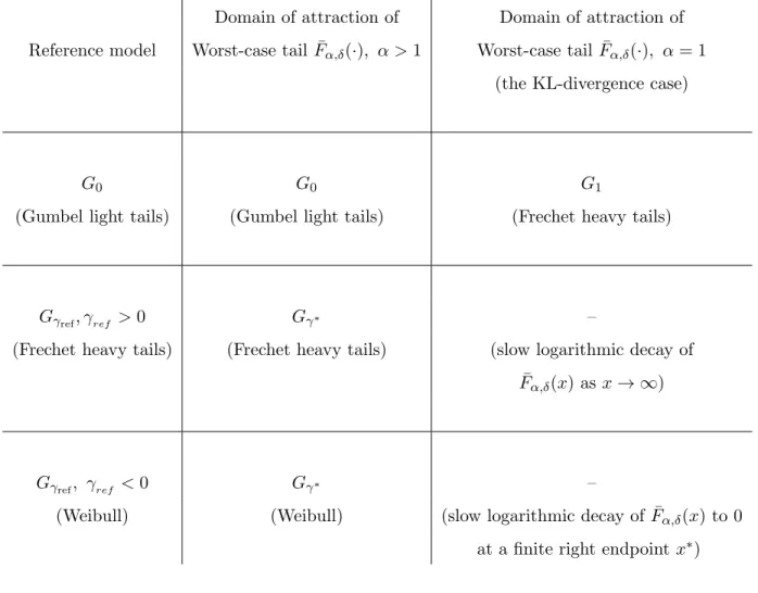
Table 2.1: A summary of domains of attraction of Fα,δ(x) = 1−F¯α,δ(x) for GEV models. Throughout the paper, γ∗ := αα−1γref
Domain of attraction of Domain of attraction of Reference model Worst-case tail ¯Fα,δ(·), α >1 Worst-case tail ¯Fα,δ(·), α= 1
(the KL-divergence case)
G0 G0 G1
(Gumbel light tails) (Gumbel light tails) (Frechet heavy tails)
Gγref, γref >0 Gγ∗ –
(Frechet heavy tails) (Frechet heavy tails) (slow logarithmic decay of ¯
Fα,δ(x) asx→ ∞)
Gγref, γref <0 Gγ∗ –
(Weibull) (Weibull) (slow logarithmic decay of ¯Fα,δ(x) to 0 at a finite right endpointx∗)
Here G← denotes the usual inverse function G←(u) = inf{x : G(x) ≥ u} with respect to distributionG.Since the framework of Section 2.3 is limited to optimization over objective functionals in the form of expectations (as in (2.11)), it is immediately not clear whether the supremum in (2.19) can be evaluated using tools developed in Section 2.3. Therefore, let us proceed with the following alternative: First, compute the worst-case tail distribution
¯
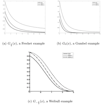
Figure 2.1: Comparison of ¯Fα,δ(x) for different GEV models: The solid curves represents the reference model Gγref(x) for γref = 1/3 (top left figure), γref = 0 (top right figure) and
γref = −1/3 (bottom figure). Computations of corresponding ¯Fα,δ(x) are done for α = 1
(the dotted curves), andα= 5 (the dash-dot curves) withδfixed at 0.1. The dotted curves (corresponding toα= 1,the KL-divergence case) conform with our reasoning that ¯Fα,δ(x) have vastly different tail behaviours from the reference models when KL-divergence is used.
(a)G1
3(x),a Frechet example (b) G0(x),a Gumbel example
(c) G−1
3(x),a Weibull example
over all candidate models, and compute the corresponding inverse
Fα,δ←(pn) := inf{x: 1−F¯α,δ(x)≥pn}.
The estimate ˆxp (defined as in (2.19)) is indeed equal to Fα,δ←(pn),and this is the content of Lemma 2.1.
Lemma 2.1. For every u∈(0,1), Fα,δ←(u) = sup{G←(u) :Dα(G, PGEV)≤δ}.
¯ Fα,δ(·) and Fα,δ←(·) that Fα,δ←(u) = inf x: sup G∈P G(x,∞)≤1−u = inf \ G∈P x:G(x,∞)≤1−u = inf \ G∈P G←(u),∞ = sup G∈P G←(u).
This completes the proof of Lemma 2.1.
Now that we know ˆxp =Fα,δ←(pn) is the desired upper bound, let us recall from Example 2.1 how to evaluate ¯Fα,δ(x) for any x of interest. Ifθx>1 solves
PGEV(x,∞)φα(θx) +PGEV(−∞, x)φα 1−θxPGEV(x,∞) PGEV(−∞, x) = ¯δ,
then ¯Fα,δ(x) = θxPGEV(x,∞). Though θx cannot be obtained in closed-form, given any
x >0,one can numerically solve forθx,and compute ¯Fα,δ(x) to a desired level of precision. On the other hand, given a level u ∈(0,1),it is similarly possible to compute Fα,δ←(u) by solving forx that satisfies PGEV(x,∞)<1−u and
PGEV(x,∞)φα 1−u PGEV(x,∞) +PGEV(−∞, x)φα u PGEV(−∞, x) = ¯δ. (2.20) Therefore, given α and δ, it is computationally not any more demanding to evaluate the robust estimatesFα,δ←(pn) for F←(p).
2.5.1 On specifying the parameter δ.
For a given choice of paramter α ≥ 1, there are several divergence estimation methods available in the literature to obtain an estimate ˆδ = Dα( ˆPMn, PGEV), where ˆPMn is the
empirical distribution of Mn. For our examples, we use the k-nearest neighbor (k-NN) algorithm of P´oczos and Schneider (2011) and Q.Wanget al.(2009). See also Nguyenet al. (2009),Nguyenet al. (2010),Gupta and Srivastava (2010) for similar divergence estimators. These divergence estimation procedures provide an empirical estimate of the divergence between sample maxima and the calibrated GEV model PGEV.
The specific details of thek-NN divergence estimation procedure we employ from P´oczos and Schneider (2011) and Q.Wanget al. (2009) are provided in Remark 2.3 below:
Remark 2.3. Suppose Mn,1, . . . , Mn,m are independent samples of Mn,andL1, . . . , Ll are samples from PGEV. Define ρk(i) to be the Euclidean distance between Mn,i and its k-th nearest neighbour among all Mn,1, . . . , Mn,m and similarly νk(i) the distance between Mn,i and itsk-th nearest neighbour among allL1, . . . , Ll. Thek-NN based density estimators are
ˆ
pk(Mn,i) =
k/(m−1)
|B(ρk(i))| and qˆk(Mn,i) =
k/l |B(νk(i))|,
where |B(ρk(i))| denotes the volume of a ball with radius ρk(i). Then, for a fixed α, the estimator for δ =Dα(PMn, PGEV) is given by
ˆ δ = 1 α−1log 1 m m X i=1 (m−1)ρk(i) lνk(i) 1−α · Γ(k) 2 Γ(k−α+ 1)Γ(k+α−1) , for α >1, where Γ denotes the gamma function, and
ˆ δ= 1 m m X i=1 log lνk(i) (m−1)ρk(i) , for α= 1.
For a fixed choice ofα ≥1 and desiredpclose to 1, theRob-Estimator(p, α) procedure in Algorithm 1 below provides a summary of the prescribed estimation procedure.
2.5.2 On specifying the parameter α.
To input to the estimation procedure Rob-Estimator(p, α) in Algorithm 1, one can
per-haps chooseα via one of the three approaches explained below:
1) Choose α so that the corresponding γ∗ =γ0α/(α−1) matches with an appropriate
confidence interval for the estimate γ0 : For example, if γ0 > 0 and the confidence
interval for γ0, estimated from data, is given by (γ0 −, γ0+), then we choose α
satisfying
γ0
α
α−1 =γ0+. (2.21)
See Examples 2.2 and 2.3 for demonstrations of choosing α following this approach. 2) Alternatively, one can choose α based on domain knowledge as well: For example,
In this instance, if a financial expert identifies the returns are instead heavy-tailed, then one can take α = 1 to account for the imperfect assumption of Gaussian tails. See Example 2.4 for a demonstration of choosingα based on this approach.
3) One can also adopt the following approach that mimicks the cross-validation
proce-Algorithm 1 To compute a robust upper bound ˆxp for VaRp(X)
Given: N independent samples X1, . . . , XN of X, a level p close to 1, and a fixed choice α≥1.
procedure Rob-Estimator(p, α)
Initialize n < N,and let m=bNnc.
Step 1 (Compute block-maxima): Partition X1, . . . , XN into blocks of size n, and compute the block maxima for each block to obtain samples Mn,1, . . . , Mn,m of maxima Mn.
Step 2 (Cali