Abstractions in Reasoning for Long-Term Autonomy

(1)

University of Massachusetts Amherst

ScholarWorks@UMass Amherst

Doctoral Dissertations

Dissertations and Theses

July 2019

Abstractions in Reasoning for Long-Term Autonomy

Kyle Hollins Wray

University of Massachusetts Amherst

Follow this and additional works at: https://scholarworks.umass.edu/dissertations_2

Part of the Artificial Intelligence and Robotics Commons

Recommended Citation

Wray, Kyle Hollins, "Abstractions in Reasoning for Long-Term Autonomy" (2019). Doctoral Dissertations. 1642.

https://scholarworks.umass.edu/dissertations_2/1642

This Open Access Dissertation is brought to you for free and open access by the Dissertations and Theses at ScholarWorks@UMass Amherst. It has been accepted for inclusion in Doctoral Dissertations by an authorized administrator of ScholarWorks@UMass Amherst. For more information, please contact

(2)

ABSTRACTIONS IN REASONING FOR LONG-TERM AUTONOMY

A Dissertation Presented by

KYLE HOLLINS WRAY

Submitted to the Graduate School of the

University of Massachusetts Amherst in partial fulfillment of the requirements for the degree of

DOCTOR OF PHILOSOPHY May 2019

(3)

c

(4)

ABSTRACTIONS IN REASONING FOR LONG-TERM AUTONOMY

A Dissertation Presented by

KYLE HOLLINS WRAY

Approved as to style and content by:

Shlomo Zilberstein, Chair

Joydeep Biswas, Member

Roderic A. Grupen, Member

Benjamin M. Marlin, Member

Weibo Gong, Member

Stefan J. Witwicki, Member

James Allan, Chair of the Faculty

(5)

ACKNOWLEDGMENTS

It is difficult for me to convey my gratitude to everyone that has contributed to my experience here in Amherst. I am grateful for the amazing experience it has been. I will always cherish the fond memories shared among friends, colleagues, and mentors. With much pleasure, I take this brief opportunity to thank many of the people who have helped shape my journey.

Shlomo Zilberstein, my advisor, has been a constant source of knowledge and inspiration. He has always encouraged me to pursue my own passions in research and has given me the freedom to do so, providing direction when it was needed. Through his guidance, conducting research has become an endlessly enjoyable and productive experience. I could not have asked for a better mentor. Thank you, Shlomo, for these great years.

I would also like to thank my committee members, who have all been very helpful. Joydeep Biswas provided insightful ideas on many occasions. He encouraged a high standard of work, which I always appreciate and respect. Rod Grupen has continually been a supportive teacher and collaborator who welcomed me into his lab and helped introduce me to robotics. Ben Marlin has been a fantastic teacher and mentor. I appreciated his thoughts on the graphical model presented in this dissertation. Weibo Gong provided great feedback throughout each stage of the dissertation process.

The team at the Nissan Research Center in Silicon Valley has been among the most supportive and fun groups I have had the privilege to work with. Stefan Witwicki, who also served on my committee, has been an amazing collaborator. I am fortunate and grateful to have worked with such a supportive and intelligent researcher. Thank you to everyone at Nissan, including director Maarten Sierhuis as well as Atsu Kobashi, Liam Pedersen, Kathy Sun, and Kelsie Zhao, who have contributed to actualizing my research on an autonomous vehicle.

Some of the most enjoyable moments during my time here have been with my fellow labmates in the Resource-Bounded Reasoning Lab. Luis Pineda and Sandhya Saisubramanian have been both productive collaborators and close friends. They have most certainly made me a better researcher and person. I will greatly miss our discussions. I am also thankful for the other fantastic members of RBR, including: Connor Basich, Rick Freedman, Shuwa Miura, John Peterson, Justin Svegliato, and Xiaojian Wu, all of whom were great colleagues and friends.

(6)

I would like to thank Michele Roberts for her support and professionalism in grant-related mat-ters, and Leeanne Leclerc for her exceptional work and advice over the years, without which I would not have navigated the complex graduate processes, nor would I have met many of my close friends. During my time here, I have met many wonderful friends and housemates. Dirk Ruiken, in particular, has been an exceptional friend, colleague, and housemate. It was only through his guidance that I was able to earnestly pursue robotics. My current housemates Matteo Brucato, Samer Nashed, and Justin Svegliato are also great colleagues and close friends. With these four housemates, I have shared countless hours of meals, games, road trips, laughs, and discussions. Thank all of you for the wonderful memories and heartfelt camaraderie at Gray Street.

Other wonderful friends with whom I have shared many great memories are: Garrett Bernstein, Su Lin Blodgett, Marc Cartright, Ilene Cartright, Orion Cartright, Sebastian Cartright, Kaleigh Clary, Joe Collard, Sally Craig, Hanifa Darwish, Francisco Garcia, Brendan Gavin, Tom Goldstein, Emily Harrington, Mitch Hebert, Tom Hooper, Sam Huston, Myungha Jang, Niri Karina, Yoonheui Kim, Li Yang Ku, Tina Kuksin, Mike Lanighan, Tiffany Liu, Katerina Marazopoulou, Jess McIver, Tamara Mercanti, Annamalai Natarajan, Pinar Ozisik, Sadegh Rabiee, Shiraj Sen, Takeshi Taka-hashi, Phil Thomas, John Vilk, Sofya Vorotnikova, and Kevin Winner. Thank all of you for making the past years memorable.

This dissertation would not have been possible without the support of my family who have always encouraged me to reach for my dreams. My parents, Robin Wray and Peter Wray, are among the most wisest, most loving, and talented people that I know. Thank you both so much for the values you have instilled in me and for your continued support throughout my life. My wife, Sajia Darwish, has brought a light to my life that I never knew possible. This dissertation was written with her by my side. Thank you Sajiajanem for your eternal love, care, and support. I look forward to our lifelong journey together.

(7)

ABSTRACT

ABSTRACTIONS IN REASONING FOR LONG-TERM AUTONOMY

MAY 2019

KYLE HOLLINS WRAY

B.S., THE PENNSYLVANIA STATE UNIVERSITY B.S., THE PENNSYLVANIA STATE UNIVERSITY M.S., THE PENNSYLVANIA STATE UNIVERSITY M.A., THE PENNSYLVANIA STATE UNIVERSITY M.S., UNIVERSITY OF MASSACHUSETTS AMHERST Ph.D., UNIVERSITY OF MASSACHUSETTS AMHERST

Directed by: Professor Shlomo Zilberstein

The path to build adaptive, robust, intelligent agents has led researchers to develop a suite of powerful models and algorithms for agents with a single objective. However, in recent years, attempts to use this monolithic approach for an ever-expanding set of real-world problems have illuminated its inability to scale, resulting in a fragmented collection of hierarchical and multi-objective models. This trend continues into the algorithms as well, as each approximates an optimal solution in a different manner for scalability. These models and algorithms represent an attempt to solve pieces of an overarching problem: how can an agent explicitly model and integrate the necessary aspects of reasoning required for long-term autonomy?

This thesis presents a general hierarchical and multi-objective model called apolicy network that unifies prior fragmented solutions into a single graphical decision-making structure. Additionally, the underlying notion of a policy, which is used by all algorithms to describe internal agent state and action, is generalized and unified in this thesis undercontroller family policies.

Policy networks are broadly useful to solve numerous real-world problems including: (1) an au-tonomous vehicle’s (AV) intersection decision-making, semi-auau-tonomous route planning with prov-able notations of safety, and capability to balance multiple objectives; and (2) a home healthcare

(8)

robot’s reasoning about multiple delivery and monitoring tasks. This thesis presents solutions to both of these distinct problems, with policy networks serving as their shared framework, each acting as part of the overall solution for rich, real-world, scalable decision-making in long-term autonomy. Reasoning about multiple objectives is common in many real-world domains due to necessary trade-offs among objectives such as solution cost, quality, and time. This thesis considers a general model oftopologically ordered objectives in decision-makingwith a preference ordering over objectives induced by a directed acyclic graph and a slack term—allowable deviation from optimal—for each objective. It is applied to AV route planning, which minimizes travel time with slack to improve time autonomous. Topologically ordered objectives in decision-making serve as a demonstration of policy constraints—multiple models, with identical state-action spaces, in a graph of constraints—within a policy network.

To achieve long-term autonomy deployed in the real world, periods of semi-autonomy will be necessary for safety and to expand the agent’s capabilities beyond what it can do autonomously. Thus, control will need to be safely transferred to a human for approval or even direct control. This thesis considers a formal framework for semi-autonomous systems that explicitly models varying levels of human or agent assistance and safely transfers control among them. It is applied to semi-autonomous vehicles for street-level route planning with proactive transfer of control, given only some of the roads are capable of autonomy, with provable notions of safety. Semi-autonomous systems serve as a demonstration of policy abstractions—multiple models, with differing state-action spaces, that transfer control among themselves—within a policy network.

Finally, a central challenge in long-term autonomy is the ability to manage multiple decision-making problems, perhaps simultaneously, that are unspecified a priori, each with differing state spaces and objectives. This thesis considers a solution for solvingmultiple online decision-components

with interacting actions (MODIA)with integrated learning to customize each decision-making

sce-nario over time for ever-improving performance. It is applied to an AV interacting with other vehicles and pedestrians at intersections and demonstrated on a fully operational AV prototype acting on real public roads. MODIA serves as a demonstration of an indefinite number of models—multiple models, with differing state spaces but identical action spaces, the quantity of which is finite but unknown a priori—within a policy network.

(9)

5. MULTI-OBJECTIVE DECISION-MAKING . . . .83 5.1 Introduction . . . 83 5.2 Topological MDP . . . 86 5.2.1 Optimality Criterion . . . 87 5.2.2 Lexicographic MDP . . . 89 5.2.3 Stationarity . . . 90 5.2.4 Graphical Representation . . . 90 5.3 Topological POMDP . . . 91 5.3.1 Optimality Criterion . . . 93 5.3.2 Lexicographic POMDP . . . 94 5.4 Algorithm . . . 95 5.4.1 Duality in Algorithms . . . 96 5.4.2 Infeasibility . . . 96 5.4.3 Optimal Algorithm . . . 97

5.4.4 Finite State Controller Algorithm . . . 98

5.4.5 Local Action Restriction Algorithm . . . 99

5.5 Application to Autonomous Vehicles . . . 100

5.5.1 Problem Definition . . . 101

5.5.2 Multi-Objective AV Route Planning Formulation . . . 101

5.6.1 Analysis of Algorithms . . . 105

5.6.2 Policy Network Representation of TMDPs . . . 111

5.7 Evaluation . . . 112 5.8 Conclusion . . . 115 6. SEMI-AUTONOMOUS SYSTEMS. . . .116 6.1 Introduction . . . 116 6.2 Semi-Autonomous Systems . . . 118 6.3 Transfer of Control . . . 121 6.3.1 Problem Definition . . . 121

6.3.2 Transfer of Control POMDP Formulation . . . 122

6.4.1 Problem Definition . . . 124

6.4.2 Semi-Autonomous Vehicle Formulation . . . 125

6.5.1 Policy Network Representation of SAS . . . 131

(12)

7. SCALABLE ONLINE DECISION-MAKING . . . .135

7.2 Multiple Online Decision-Components with Interacting Actions . . . 137

7.2.1 Decision-Making with MODIA . . . 137

7.2.2 The MODIA Executor . . . 139

7.2.3 The MODIA Objective . . . 139

7.2.4 LEAF for MODIA . . . 140

7.2.5 Risk-Sensitive MODIA . . . 141

7.4.1 Policy Network Representation of MODIA . . . 145

7.5.1 Experiments in an Industry-Standard Simulation Environment . . . 147

7.5.2 Experiments on a Fully Operational AV Prototype . . . 148

7.5.3 Discussion . . . 149 7.6 Conclusion . . . 150 8. CONCLUSION. . . .157 8.1 Future Work . . . 157 8.2 Final Thoughts . . . 159 BIBLIOGRAPHY . . . .160

(13)

LIST OF TABLES

Table Page

3.1 The problem sizes and run times for each model. . . 65 4.1 A general NLP formulation using an unconstrained controller family policy for

POMDPs. . . 72 4.2 Results using new policy form with same NLP algorithm and same number of FSC

nodes (|N|). Metrics: Time (seconds, 10 trials) and average discounted reward

(ADR, 100 trials). Bold indicates statistically significant improvement. . . 80 5.1 An NLP using an FSC to approximate_{SolveRelativeCMDP}(·) in

Algorithm 2. . . 98 5.2 LMDP problem domain sizes (|S|and|A|) and run times (CPU and GPU) for

autonomous vehicle LMDP experiments over 10 cities using real-world data from OpenStreetMap. . . 113 5.3 LPOMDP problem domain sizes (|S|,|A|, and |Ω|), the value following the policyπ

at initial beliefs ( ˆV_iπ(b0)), and run times (CPU and GPU) for autonomous vehicle LPOMDP experiments over 10 cities using real-world data from

OpenStreetMap. . . 114 6.1 Results for SAVE experiments on 10 cities for human driverλ, autonomous vehicle

ν, and the human semi-autonomous vehicle collaboration λ&ν drivers. Metrics: goal reachability ‘G’, autonomous driving percentage ‘%’, and travel time ‘T’

(seconds). . . 134 7.1 Results for 6 intersection problems described by the number of road segments (RS),

vehicles (V), pedestrians (P), and potential incidents (PI). Metrics: time to complete intersection (seconds) for MODIA AVM(including the number of

(14)

LIST OF FIGURES

Figure Page

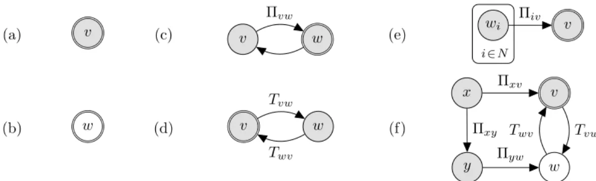
3.1 Basic examples of the graphical notation described in Section 3.4.1 that is used to represent policy networks, with eachv∈V following some model

v∼MDP(Sv, Av, Tv, Rv): (a) stationary vertex; (b) non-stationary vertex; (c) constraint edge; (d) transfer of control edges; (e) plate notation for a set ofN

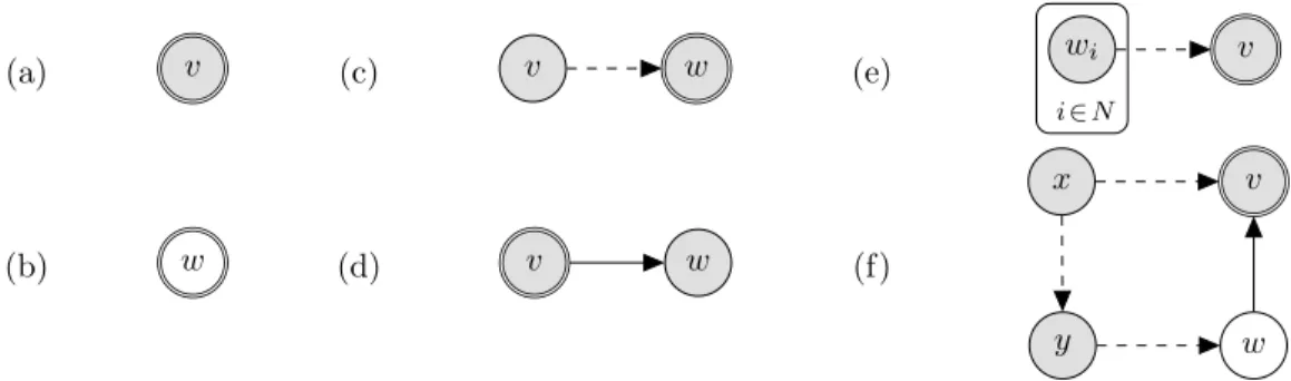
constraints; and (f) mixture of the concepts. . . 37 3.2 Similar basic examples as shown in Figure 3.1 of thealternate graphical notation

described in Section 3.4.2 that is used to more quickly represent policy networks. Eachv∈V follows some modelv∼MDP(Sv, Av, Tv, Rv): (a) stationary vertex; (b) non-stationary vertex; (c) constraint edge; (d) transfer of control edge; (e) plate notation for a set ofN constraints; and (f) mixture of the concepts.

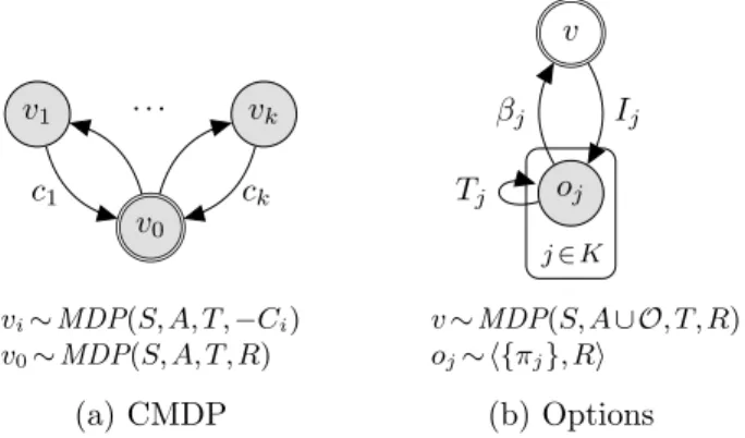
Conveniently this alternate form explicitly defines the dependency graph. . . 53 3.3 Two examples of policy networks: (a) a constrained MDP, traditionally for a

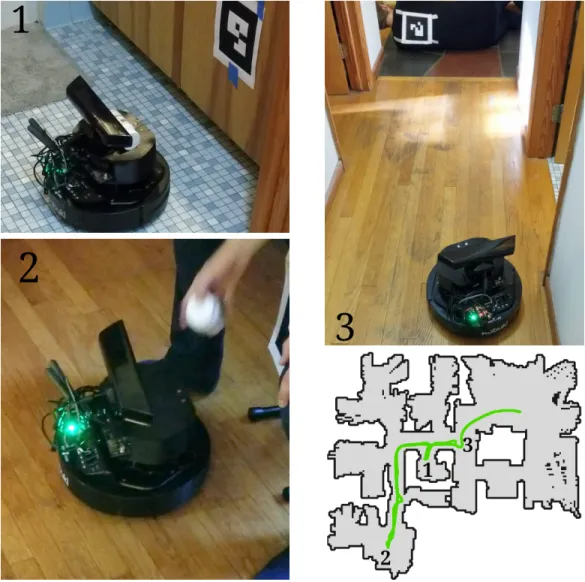
planning agent; and (b) the options framework, traditionally for a reinforcement learning agent. . . 59 3.4 The policy network for the home healthcare robot. . . 64 3.5 Experiments with the home healthcare robot using this policy network in the real

household shown above. Three highlights are shown: (1) medicine retrieval for taskt1, (2) medicine delivery completion with transfert1→h→t2, and (3)

interruption of cleaning taskt2 by detecting a fall with taskfi and calling for

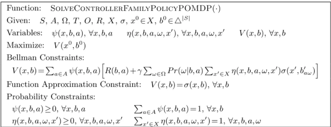
assistance. . . 68 4.1 Robot experiment. Path: FSC (blue), belief (green) actions. . . 81 5.1 Basic examples of the graphical notation that is used to represent a TMDP’s

topological constraints, for each reward vertexi∈K. The examples shown are: (a) an MDP before solving it; (b) an MDP after solving it; (c) a simple

two-reward LMDP; (d) a simple two-constraint CMDP; (e) plate notation for a set ofK0=K− {k}constraints; and (f) mixture of the concepts for a set of

K00=K− {1,2, k} constraints. . . 91

5.2 Examples of action restriction and slack affordance. The true value functions (gray dotted lines) are approximated by theα-vectors from below (black lines). The first value functionV1(left) is reduced up to the slackδ1to afford the second

value functionV2(right) to greatly increase its value. This example illustrates

LVI’s operation. . . 95 5.3 LMDP (left), CMDP (center), and an example tree graph TMDP (right)

(15)

5.4 Example LMDP policy for Denver (top), Austin (center), and San Francisco

(bottom) with driver attentive (left) and tired (right). . . 113 5.5 Example LPOMDP policy for Boston with driver belief 0.2 (left) and 0.8 (right). . . 114 6.1 SAS represented as a policy network. . . 132 6.2 Example SAVE policy with TOC in Boston (left) and a TOC POMDP in SAVE

simulator (right). . . 133 7.1 Example visualization of MODIA for AVs. Offline, the DPs (left) are solved:

vehicles (P1) and pedestrians (P2). Online, the AV approaches an intersection in

the environment (center). DCs (right) are instantiated from DPs based on 3 new observations: 2 vehicles (C1 andC2) and 1 pedestrian (C3). Each DC

recommends an action (¯a): 2 stops and 1 go. The executor decides: stop. The agent takes the action, resulting in regret forC2’s action inRt. New observations induce DC updates. . . 138 7.2 MODIA represented as a policy network. . . 146 7.3 Our fully-operational AV prototype at a 4-way stop intersection that implements

AV MODIA and LEAF. . . 150 7.4 Experiment3-Way Stop (Part 1 of 2) in Sunnyvale, California during 2017. This is

MODIA, as part of a policy network, interacting with real traffic on a public road. The left corner shows a visual of the high-level route plan. The right corner shows a visual of the mid-level MODIA decision-making; each row represents one DC. Images provided courtesy of Nissan Research Center - Silicon Valley. . . 151 7.5 Experiment3-Way Stop (Part 2 of 2) in Sunnyvale, California during 2017. This is

MODIA, as part of a policy network, interacting with real traffic on a public road. The left corner shows a visual of the high-level route plan. The right corner shows a visual of the mid-level MODIA decision-making; each row represents one DC. Images provided courtesy of Nissan Research Center - Silicon Valley. . . 152 7.6 Experiment4-Way Stopin Mountain View, California during 2017. This is MODIA,

as part of a policy network, interacting with real traffic (left vehicles) and one staged researcher (center vehicle). Images provided courtesy of Nissan Research Center - Silicon Valley. . . 153 7.7 ExperimentPartially Observable T-Intersection (Part 1 of 2) in Sunnyvale,

California during 2017. This is MODIA, as part of a policy network, acting on real public roads with one staged researcher (partially observable left vehicle). The left column shows the front view and the right column shows the side view. Images provided courtesy of Nissan Research Center - Silicon Valley. . . 154 7.8 ExperimentPartially Observable T-Intersection (Part 2 of 2) in Sunnyvale,

California during 2017. This is MODIA, as part of a policy network, acting on real public roads with one staged researcher (partially observable left vehicle). The left column shows the front view and the right column shows the side view. Images provided courtesy of Nissan Research Center - Silicon Valley. . . 155

(16)

7.9 Experiment4-Way Stop With Pedestrian in Mountain View, California during 2017. This is MODIA, as part of a policy network, interacting with two staged

researchers (vehicle and pedestrian). Images provided courtesy of Nissan

(17)

CHAPTER 1

INTRODUCTION

Autonomous systems have been successfully deployed in a wide variety of applications ranging from space exploration [147], water reservoir control [23], smart wheelchairs [116], energy conserva-tion [75], home healthcare robots [139], and autonomous vehicles [134]. Long-term autonomy (LTA) has arguably always been the goal of many of these autonomous robotic agents. Generally, LTA refers to an agent that is able to be “deployed for extended periods in real-world environments” [71] and “adapt to changes in the environment in order to remain autonomous” [11]. LTA solutions must provide a “tight integration of a number of autonomous components, including a symbiotic human-robot relationship” [11], such that “integrating state-of-the-art artificial intelligence and human-robotics research” will “increase their robustness” [54]. Consequently, “LTA systems inherently present an integration challenge, particularly when different AI abilities need to work together” [71]. This includes reasoning about “localisation and navigation; object and/or person perception; plus task planning and/or scheduling” [71]. Due to the sheer complexity of such systems, it is only recently becoming a reality to deploy these kinds of agents at a large scale so as to directly interact with the day-to-day lives of individuals.

One of the most prominent recent applications of long-term autonomy is autonomous vehicles (AVs). They serve as the motivating domain for much of the work contained in this thesis. AVs must be able to drive autonomously the majority of the time in both highways and urban environments. They must reliably perform the complex merges, lane changes, yields to oncoming traffic, cautious edges forward for visibility, and negotiations with vehicles, bikes, and pedestrians at a diverse array of intersections. In this thesis, we call these kinds of tasks mid-level decision-making to differentiate it from so called high-level route planning (e.g., GPS navigation) and low-level path planning (e.g., millimeter precision control of the wheels). In other words, mid-level reasoning considers the “task planning and/or scheduling” and incorporates partial observability models for “object and/or person perception.” The low- and high-level reasoning considers the “localisation and navigation” of the steering wheel and for the overall route, respectively. Reasoning at these levels should be tightly integrated in order to increase the AV’s robustness. All three levels arguably can also entail more

(18)

than one objective, as AV passenger safety, external vehicle and pedestrian safety, time to reach a destination, and even social acceptability, must all be prioritized and reasoned about for each decision made. Moreover, a human that can monitor the AV is typically required by law, namely the driver, such that a “symbiotic human-robot relationship” must be part of the integrated solution, with a safe transfer of control between the two. AV research overall has advanced rapidly since the DARPA Grand Challenge [127], which acted as a catalyst for subsequent work on low-level sensing [120, 111] and control [74, 35], as well as our recent work on mid-level decision-making [134] and high-level semi-autonomous route planning [132], both discussed within the thesis. These growing lines of research have highlighted the inability for a monolithic model—that is, a massive model with one large state-action space and one objective—to alone tractably capture all necessary aspects of reasoning.

1.1

Models of Reasoning

This thesis focuses specifically on the principled formulation and integration of these reasoning aspects—for example, the low-, mid-, and high-level AV reasoning—towards the goal of long-term autonomy, using theMarkov decision process (MDP)[8, 55] as a foundation. An MDP consists of four components to describe the necessary pieces to make decisions sequentially over time. First,states

describe what information is important, such as locations of the AV and other vehicles. Second,

actions describe what the agent can do, such as stop or go forward. Third,transitionsdescribe how the world’s state changes after an action is performed, such as how going forward advances the AV’s location. Fourth, rewards describe which states and actions are good or bad for the agent, such as how it is good to arrive at the AV’s destination. At each state, the agent chooses an action to perform. We call this decision-making assignment of state to action apolicy. These components, or equivalent representations, form the mathematical foundation on top of which the vast majority of planning and learning techniques are built within artificial intelligence research.

As discussed above, for real-world applications such as AVs, a large monolithic MDP simply cannot tractably capture the diverse array of tasks that a long-term autonomous agent inevitably encounters in the environment. Fortunately, many techniques that extend the MDP can address some of the key challenges found in designing the reasoning components for long-term autonomous agents. Hierarchical methods such as the options framework [122], hierarchical abstract machines [87], or macro-actions [53] allow for different compositions of hierarchical policies the agent follows. While this enables tractable solutions to be implemented, each approach has benefits and drawbacks with-out a unified view abwith-out how these hierarchical solutions operate. Multi-objective methods allow for

(19)

a single task to consider many objectives simultaneously (e.g., quality, cost, and time), and includes scalarization approaches [103], constrained MDPs [2], and lexicographic MDPs [135]. While this enables more than one objective to be considered, each approach again has benefits and drawbacks, without a unified view regarding their relation. Moreover, these multi-objective methods only allow for reasoning about the same state and action spaces—the scope of the problem space is identi-cal, with only the description of objective differing. Applications such as AVs require reasoning

simultaneously about multipledistinct tasks or problems, perhaps with different concepts of state and action, such as when there are any number of vehicle and pedestrian interactions present [134]. Lastly, such applications of long-term autonomy can greatly benefit from human feedback and col-laboration to further empower the agent to complete its objectives [132]. With all of these pieces available to solve the reasoning problems in an agent with long-term autonomy, no technique exists to easily integrate them. The need for a unified model to simultaneously handle all of these necessary aspects of reasoning for long-term autonomy motivates the approaches contained in this thesis.

1.2

Models of Reasoning in Long-Term Autonomy

Inspired by the need for mathematically principled solutions to scalable reasoning models in long-term autonomy, and building off of the established hierarchical and multi-objective work, this thesis presents apolicy network. The overall idea is simple and intuitive: (1) break the big problem into small pieces, and (2) represent how the small pieces relate to one another.

For example, consider driving between home and work repeatedly everyday. Each day is different and each individual trip can take a long time even by itself. It is impossible to reasonat the same time about all interactions with all vehicles we might encounter at all traffic light, stop sign, and yield intersections; every millimeter of control for the wheels at all places; all pedestrians that may cross our path; and all possible roads we could traverse. Instead, we reason and learn about solutions to each small piece separately, with a holistic understanding how each piece relates to others. The combination of these pieces enables us to solve the larger problem and drive between home and work repeatedly everyday.

In a policy network, we define each of these small pieces with its by its own policy space for a reward, describing concerns only related to that task. We then relate these small pieces to one another. For example, one task can constrain what another can do by limiting its policy space, or one task can leverage another as a subtask by temporarily transferring control to it.

(20)

Each chapter presents a focused exploration of a novel aspect of a policy network. Moreover, they describe how it can be used as one of these pieces of the holistic solution to AVs. Chapter 4 explores a generalized notion of policy within a policy network. Chapter 5 explores a graph-based preference structure among different objectives in a policy network. Chapter 6 explores the transfer of control among different models in a policy network. Chapter 7 explores the simultaneous interaction of multiple different models in a policy network. These aspects, when combined, aim to provide a holistic representation of many key reasoning aspects towards the goal of long-term autonomy, specifically focused on the motivating autonomous vehicle domain.

1.3

Contributions

This thesis unifies the numerous models and their policy representations for constructing intelli-gent aintelli-gents with long-term autonomy. Additionally, it presents solutions to three critical components within such agents: incorporating multiple objectives, leveraging human assistance for safety, and fusing multiple models online for scalable long-term autonomy. We present solutions to autonomous vehicle reasoning and demonstrate success on a true autonomous vehicle prototype.

Policy Networks This thesis presents a single formal unified model that encapsulates hierarchical and multi-objective decision-making: policy networks. We provide complete novel formal proofs for various prior models (e.g., options and constrained MDPs) as well as the three new models presented within this thesis. A novel general algorithm to solve policy networks is described and analyzed. Numerous examples and illustrations are provided to properly illuminate the nuances of policy networks as a new solution to long-term autonomous systems. A home healthcare robot domain is fully explained, implemented, and evaluated on a real robot to demonstrate the effectiveness of policy networks to solve real-world problems.

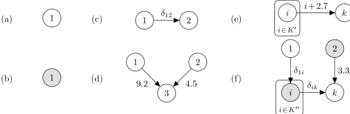
Controller Family Policies In addition to the unified view of models, this thesis unifies the policy and value formulations used by state-of-the-art algorithms: controller family policies. We provide complete novel formal proofs that the POMDP policies used by these algorithms are actually instances of the controller family representation. We present a novel controller family policy for POMDPs as well: belief-infused finite state controllers. This approach is demonstrated and analyzed in both simulation on standard benchmark domains and on a real robot acting in the world.

Multi-Objective Decision-Making A novel form of multi-objective model called a topological MDP (TMDP) is described, as well as algorithms that scalably solve TMDPs. A theoretical analysis

(21)

of its properties is provided, with proofs showing that it generalizes lexicographic and constrained MDPs. These models are analyzed on a semi-autonomous vehicle route planning domain using real-world road data.

Semi-Autonomous Systems The novel formal definition of a semi-autonomous system (SAS), including important properties such as strong and transfer of control, is provided. It describes a form of provably safe shared control of a robot between any number of agents and humans. A novel semi-autonomous vehicle domain is presented that implements the SAS model and its transfer of control process. A theoretical analysis shows that it preserves this form of provably safe shared control. Experiments are provided, which use real public road data, illustrating the benefits of the SAS formulation.

Scalable Online Decision-Making A novel formulation called MODIA is presented that al-lows for multiple decision-making components to simultaneously be active and control the system together. This enables scalability and the ability to handle an unknown a priori number of simul-taneous problems encountered. Formal definitions, theoretical analysis, and integration of learning are described in detail. This novel theoretical formulation is analyzed within the context of inter-section, pedestrian, lane change, merge, and pass obstacle scenarios for long-term deployments of autonomous vehicles in urban and highway settings. This is implemented on a fully operational autonomous vehicle acting on real public roads.

Autonomous Vehicle Decision-Making Throughout this thesis, we use autonomous vehicles for our motivation and experimentation, as it is the first major example of long-term autonomy within society. As a result, the combination of the solutions presented in each chapter offers a strong overall solution for autonomous vehicle decision-making. The actual design and full implementation on autonomous vehicles clearly demonstrates that our approaches are successful at solving the important decision-making problems for one of the first long-term autonomous systems acting in society.

1.4

Outline

Chapter 2 introduces the core concepts used throughout the thesis. Specifically, it introduces the notion of an MDP and a POMDP, as well as numerous variants. The various forms of policy—that is, how the agent plans to behave in its environment—are covered, in addition to the core algorithms used for each model and policy form. It concludes with a discussion of the relevant hierarchical and multi-objective models as well as other solutions to address scalability in autonomy.

(22)

Chapter 3 formally defines policy networks with detailed explanations and formal proofs that prior related work are instances of policy networks. It also presents an algorithm and analyzes its characteristics. It is evaluated on a home healthcare robot domain and demonstrated on a real robot. The following three subsequent chapters include a formal mapping of the chapter’s model to a policy network.

Chapter 4 describes controller family policies as a unifying framework for the policy and value representations used by algorithms to solve POMDPs and its variants. Formal proofs that prior policy forms, such as belief point-based, finite state controller (FSC), and compression methods, are all members of the controller family. A new policy form is presented for POMDPs, with experiments that show it can improve the performance of a POMDP solver and an evaluation on a real robot.

Chapter 5 describes the process handling multiple objectives as a directed acyclic graph with slack constraints including a detailed theoretical analysis and approximate algorithms. Detailed solutions which use them are presented for autonomous vehicles.

Chapter 6 formalizes the notion of semi-autonomous systems (SAS), including the definition of a strong SAS—a notion of safety—as well as a formal description of learning to improve autonomy over time. Detailed solutions which use them are presented for semi-autonomous vehicles.

Chapter 7 presents a formal model that allows multiple decision-making models to be simulta-neously active, each essentially recommending an action with an executor model making the final decision. This enables a single agent to handle an unknown a priori number of simultaneously en-countered scenarios and/or entities in the world. We define properties of this model and a special class of solution that works well in practice. We demonstrate successful implementation in simulation and on Nissan’s fully operational AV prototype acting in real intersections on public roads.

Chapter 8 takes a step back and examines all of the techniques presented in the thesis: policy networks, controller family policies, TMDPs, SAS, and MODIA. Conclusions are drawn about what has been accomplished, how this fits into the broader research community, and where this line of work is heading. It concludes with final thoughts on the wide array of novel solutions presented within the thesis toward the goal of agents with long-term autonomy.

(23)

CHAPTER 2

BACKGROUND

In this chapter, we introduce the foundational definitions of sequential decision-making models and the core algorithms that solve them in practice. We begin with the Markov decision process (MDP) and discuss related fully observable models. Next, we cover the partially observable MDP (POMDP) and the numerous algorithms used to solve them approximately. The MDP and POMDP serve as the primary models used throughout the thesis. Lastly, we cover relevant hierarchical and multi-objective techniques as well as other general approaches that address scalability in decision-making.

2.1

Markov Decision Process (MDP)

The MDP was created in the 1950’s with its notions of optimality given by Bellman [8] and additional refinements by Howard [55]. The model defines a set of relevant states and actions to a decision-maker. At each time step, an action is performed causing the state to update to a successor state following a stochastic process. This stochastic process is said to have theMarkov property—the next state only depends on the current state and action performed, not any other state visited in the past. Immediate rewards are given to this decision-maker at each time step. While a few notions of objective exist, they each seek to maximize a notion of expected reward experienced over time.

This thesis primarily focuses on a class of MDP: discrete time, finite state, and finite action over an infinite horizon with discounting starting from an initial state. This is a modern artificial intelligence perspective on MDPs. Thus, the notation and definitions for the MDP model is first presented with this in mind to unify the overall discussion throughout the thesis. The nuances of the other MDP definitions are discussed once this modern artificial intelligence definition is presented.

2.1.1 Formal Definition

AMarkov decision process (MDP)[8] is a sequential decision-making model defined by the tuplehS, A, T, Ri:

(24)

• A is a finite set of actions,

• T:S×A×S→[0,1] is a state transition function such that T(s, a, s0_{) =}_{P r}₍_s0_{|s, a}_{) is the}

prob-ability of successor state s0 given actionawas performed in states, and

• R:S×A→_Ris a reward function such thatR(s, a) is immediate reward for performing action ain states.

An MDP operates as a stochastic control process over discrete time steps up to a horizon h∈

N∪ {∞}. At each time step, the system is in a statesand an actionais performed. Immediately, a reward signal is generated followingR(s, a). Then, a successor states0 is stochastically generated following T(s, a, s0). This process continues until horizon his reached. An MDP policy describes which actions are performed in which states over time. This policy is then used in an objective function to describe the notion of expected reward. We consider twoobjective functions: expected reward over finite and infinite horizon.

Aninfinite horizon MDP has a horizonh=∞and a discount factorγ∈[0,1). The policy π:S→Amaps each state to an action. Let Π denote the set of all policies. The objective is to find a policyπthat maximizes the expected reward over all states:

E hX∞ t=0 γtR(st, π(st)) π i (2.1)

with st_{denoting a random variable for the state at time} _t _{generated following}_T_{. Therefore, for a} policyπ, thevalueVπ:S→Ris the expected reward at state sfollowing theBellman equation:

Vπ(s) =R(s, π(s)) +γX s0_∈_S

T(s, π(s), s0)Vπ(s0). (2.2)

It is also convenient to define the Q-value functionQπ_:_S_×A_→

Rfor statesand actiona:

Qπ(s, a) =R(s, a) +γX s0_∈_S

T(s, a, s0)Vπ(s0). (2.3)

Theoptimalpolicyπ∗∈Π is the policy that obtains the maximal valueV∗. The optimal value can be computed by theBellman optimality equation:

V∗(s) = max a∈A R(s, a) +γX s0_∈_S T(s, a, s0)V∗(s0), (2.4)

(25)

or equivalently denoted V∗(s) = maxaQ∗(s, a). The optimal policy can be extracted by π∗(s) = argmax_aQ∗₍_{s, a}_{). Equation 2.4 is a contraction operator on the Banach space of value functions}

with the max norm metric and Lipschitz constant γ. It computes the unique fixed point following Banach’s fixed point theorem. This is an important property with infinite horizon objectives, as there is exactly one unique fixed point in value. Additionally, to obtain these optimal values over time, a policy need not also be dependent on the time step. For a given objective, if its policies have this property then they are called stationary. There exist optimal stationary policies for infinite horizon MDPs [12]. If this were not the case, then it might require infinite memory to store the policy over time.

A finite horizon MDP has horizon h∈N and time steps denotedT ={1, . . . , h}. In the finite horizon case, optimal policies are oftennon-stationary. Thus, the policy π:S× T →A maps states and the current time to an action. Similarly, the objective is to find a policyπthat maximizes the expected reward over all states and time:

E h_Xh t=0 γtR(st, π(st, t)) π i . (2.5)

The value functionVπ:S× T →Rat time tfor state stis:

Vπ(st, t) =R(st, π(st, t)) + X st−1_∈S

T(st, π(st, t), st−1)Vπ(st−1, t−1) (2.6)

withVπ(s,0) = 0. The Bellman optimality equation to computeV∗ follows in the natural way:

V∗(st, t) = max a∈A R(st, a) + X st−1_∈_S T(st, a, st−1)V∗(st−1, t−1). (2.7)

2.1.1.1 Important Related Terminology

The objective function in Equation 2.1 requires that all states maximize expected utility over time given a single policy. In many problems, we know the starting state of the system and do not need to plan for all possible states. This can be exploited to great effect in terms of performance and memory usage. It is also necessary for tractability in continuous or otherwise infinite state spaces. We call this aninitial states0_∈_S_{. Hereafter, we will assume initial state is provided.}

Also, there is the important notion of an absorbing state. A state s is called absorbing if T(s, a, s) = 1 for all actions a. This is also called a terminal state in some cases. These will be particularly useful in the next few sections.

(26)

For any initial states0, we can define ahistory¯h=hs0_{, a}0_{, s}1_{, a}1_{, . . . , a}h−1_{, s}h_i_{over some horizon} h as the sequence of states encountered and actions performed over time. Let ¯H denote the set of all histories, and ¯Hh _{denote the set of all histories of horizons 0, 1, 2, ...,} _h−_{1, and} _h_{. This is} also called atrial in some planning contexts or anepisodein some reinforcement learning contexts, though there are subtle differences. If the absorbing state is known, trials often terminate once one has been reached.

Most problem domains describe the state space S in terms of state factors S1, . . . , Sk such that S=S1× · · · ×Sk. This is opposed to a so-called flat state space representation. The action space A can also be factored in terms of action factors A1, . . . , Ak such that A=A1× · · · ×Ak. Factored representations provide no additional benefits aside from convenience. Instead, additional assumptions are required, such as independence assumptions in state transitions or reward, to allow this explicit structure to be exploited.

Finally, the application of the Bellman optimality equation, also called anupdate equation, allows us to compute aresidualerror. GivenV and aV0 resulting after an update, the residual for a state s is|V(s)−V0₍_s₎_|_{. The residual over all states is given by a}_{max norm} _kV₋_V0_k

∞= maxs|V(s)− V0(s)|. This may be used to check convergence in algorithms.

2.1.1.2 Additional Refinements

The modern use of MDPs within the artificial intelligence community has refined the definitions surrounding MDPs. For example, it is unfortunately common practice to abuse notion and put the discount factor γ in the model definition. This confuses the three distinct components: model, policy, and objective. Additionally, the distinction of finite versus infinite state or action spaces is not always mentioned, as finite is essentially assumed by default. Similarly, it is assumed discrete time by default as well. There are, however, some common refinements that arise in practice.

First, the reward function can simply depend on the state R0_:_S_→

R or depend on the state, action, and successorR00:S×A×S→R. The former is a weaker definition of reward due to the max inside the Bellman optimality equation. That is to say, given any R0, we can write the equation with R:S×A→_R instead using R(s, a) =R0(s); however, it is not always possible for R0 to be defined for an arbitraryR, without adding extra states, etc. Interestingly,R00 andRare equivalent representations due to the summation inside the Bellman optimality equation. Namely, we can rewrite one as the other following:

R(s, a) =X s0_∈_S

(27)

We choose the cleaner reward R throughout this thesis, though it might affect approximate algo-rithms that manipulate the Bellman optimality equation.

A different form of policies also exists that admits stochastic actions with π:S×A→[0,1] such thatπ(s, a) =P r(a|s). Importantly, it is proven that for all MDP models we consider, there exists a deterministic policyπ:S→Athat obtains optimal values withV∗=Vπ_{. Stochastic policies are}_not

required in general. Stochastic policies are primarily useful for approximation and online learning algorithms. However, one notable exception areconstrained MDPs, as detailed in Section 2.4.2.2, which require stochastic policies to obtain their maximal possibleV∗.

Briefly, there are two other adjustments used in practice. First, reward can be described in terms ofcost. In many cases, this refers to the negated reward. Second, without loss of generality,distinct action sets can be defined for each statesby overloading notation withA(s)⊆A.

This thesis focuses on infinite horizon MDPs since the finite horizon case can, in essence, be captured by the infinite horizon case. Concretely, letγ= 1, a state factorT for time that decrements each step, and an absorbing state when the state factor for T is 0 with a reward of 0. Technically, classical definitions of finite horizon MDPs allowed for T and R to depend on the time remaining as well, which is handled by this mapping. Note that this form still has the Markov property, as the state itself only depends on the previous state, even if time is a factor.

Finally, a third less commonly used, though equally valid, objective function exists as well: the average reward MDP. We leave this and other rare objectives to future analysis outside this thesis.

2.1.2 Stochastic Shortest Path (SSP) Problems

While MDPs are quite expressive in their own right, there is a more general formulation that is widely used. Consider an MDP in which there is no discounting and the horizon is finite but unknown a priori. We call this anindefinite horizon. Given an initial and goal state, this describes a stochastic shortest path problem.

Formally, a stochastic shortest path (SSP) problem [10] is a sequential decision-making model defined by the tuplehS, A, T, C, s0_{, s}g_i_:

• S is a finite set of states,

• T:S×A×S→[0,1] is a state transition function such that T(s, a, s0) =P r(s0|s, a) is the prob-ability of successor state s0 given actionawas performed in states,

(28)

• C:S×A→R+is a non-negative cost function such thatC(s, a) is immediate cost for perform-ing actionain states,

• s0∈S is an initial state, and

• sg∈S is a goal state withT(sg,·, sg_{) = 1 and}_C₍_sg_,_·_{) = 0 (i.e., absorbing zero-cost).}

Like MDPs, an SSP policy is defined byπ:S→A, provided it is stationary. Moreover, a stationary policy is said to be proper if the probability of reaching the goal sg _{is 1 as}_t_{→ ∞}_{. Any state in} which this probability is less than 1 is called adead end[68]. Importantly, SSP problems assume: (1) there exists a proper stationary policy, and (2) all improper stationary policies have infinite cost. Similar to an MDP, the objective is to find the policy π that minimizes the expected cost to reach the goal starting from the initial state:

E hX∞ t=0 C(st, π(st)) π, s 0i _(2.8)

with st _{denoting a random variable for the state at time} _t _{generated following} _T_{. For a policy} _π_, the valueVπ_:_S_→

Ris the expected cost at statesfollowing:

Vπ(s) =C(s, π(s)) +X s0_∈_S

T(s, π(s), s0)Vπ(s0). (2.9)

Similarly, the Bellman optimality equation is given by:

V∗(s) = min a∈A C(s, a) +X s0_∈_S T(s, a, s0)V∗(s0). (2.10)

The optimal policy is likewise extracted byπ∗(s) = argminaQ∗(s, a). Lastly, it is an operator similar to MDPs, however, it has a weighted max norm metric.

Technically, the original SSP definition allows for negative costs and a non-finite set of actions. However, the proper policy assumption must be modified, and a second assumption is needed with respect to the compactness of actions and continuity with respect toV. Also, a single initial and goal state in the SSP model automatically generalize to multiple initial and goal states. This mapping uses a zero-cost transition without discounting to trivially model any number of initial or goal states using just one of each.

In any case, this form of SSP is more general than the MDP models and objectives previously defined—that is, any finite or infinite horizon MDP with discrete time, finite state, and finite action

(29)

can be mapped to an SSP. For any MDP, simply add an initial and goal state. Assign zero cost uniform transition over all MDP states from the initial, multiply the MDP state transitions byγ for remaining in the MDP’s original state space, and assign a probability of (1−γ) for transitioning from these states to the goal. The converse mapping does not always exist, as indefinite horizon without discounting cannot be properly mapped to the aforementioned formulation of MDPs.

2.1.3 Path Planning with Harmonic Functions

Most robots have a more focused planning problem: quickly and smoothly navigate from one location to another while avoiding obstacle collisions. This domain of problems and solutions are calledpath and motion planning. For path planning used within this thesis, we consider a special kind ofpotential field methodthat employs a solution to Laplace’s equation calledharmonic functions[29, 133], fully formalized for robotics by Connolly and Grupen [30]. Among the many benefits of harmonic function solutions is their unique relation to SSPs. Due to this important relationship, we will use the SSP notation for overall consistency.

Intuitively, harmonic functionsflow from a source to a sink following physics equations that can model basic fluid dynamics. These paths or streamlines are smooth natural paths that optimally minimize the probability of hitting an obstacle while travelling to the goal. Formally, Laplace’s equation is a form of Poisson’s equation with an equality of zero. We have twice continuously differentiable functionφ:X→_Rdefined onn-dimensional region X⊂_Rn _{with boundary}_∂X_:

52_φ₌ n X i=1 ∂2_φ ∂x2 i = 0.

The solutions to Laplace’s equation are calledharmonic functions. This is solved using a bounded discrete regular sampled grid (of states) on X denoted S=S1× · · · ×Sn with eachSi={1, . . . , mi} for somemi∈N. On each grid state, we apply a Taylor series approximation, use Dirichlet boundary conditions with 1 for obstacles and 0 for goals, and apply finite (central) difference. LetG⊂Sdenote the set of absorbing goal states, andO⊂S denote the set of absorbing obstacle states. It is assumed all boundary states are either goals or obstacles. Lastly, let N(s) ={s0_∈S|s0

i=si±1∀i} be the set of all 2nneighboring grid states ofs /∈G∪O.

As in SSPs, there is a resulting system of equations acting as a value update equation. Let V:S→Rbe thevalueof each grid states /∈G∪Ofollowing:

V(s) = X s0_∈_N₍_s₎

1 |N(s)|V(s

(30)

For a goals∈G, V(s) = 0, and for an obstacles∈O, V(s) = 1. As written, this is a special case of successive over relaxation (SOR) calledGauss-Seidel. Interestingly, the optimal values correspond directly to the probability of hitting an obstacle while moving to a goal state [28].

These values determine the path the robot will take called streamlines. Streamlines are essen-tially the policy of the harmonic function with respect to the original state space X. It follows gradient descent by interpolating over the grid values and terminates early once it reaches a goal or obstacle. Formally, given an initialx0_{, a streamline of length}_τ _{is defined recursively by the locations}

hx0_{, x}1_{, . . . , x}τ_i_{induced by:}

xt+1=xt−h5φˆ(xt) (2.12)

with step sizehand ˆφ:X→Rdenoting the interpolated approximate ofφusing V∗, assuming it is normalized to a unit vector.

Other techniques exist for robotic path and motion planning. Probabilistic roadmaps (PRMs)[64] begin by randomly selecting points to create a collision-free graph. Then, it enters a query phase that connects the start and goal locations. Eventually it finds the fastest route within the final graph. Rapidly-exploring random trees (RRT) [69] randomly construct trees following any general state transition, including any non-holonomic constraints. While fast, this random exploration does not always produce the desired smooth optimal trajectories, and does not explicitly incorporate measures of obstacle avoidance. We leave these other forms of path planning to analysis in future work outside this thesis.

2.1.4 Algorithms

Solving MDPs in general is P-complete in the size of the problem in states and actions [86]. However, it is common practice to have an exponential state space defined by all permutations of state factors [77]. In any case, there are two very important optimal algorithms for MDPs that informed the decades of subsequent algorithms which followed.

Value iteration (VI) [8] applies Equation 2.4 to all states until a convergence criterion is met. A very important corollary is that these updates can be applied to any state in any order, provided no state is starved of updates (i.e., all states are sampled infinitely often as t→ ∞). This is called asynchronous VI, and it forms the foundation of the majority of approximate algorithms due to its ease to prove convergence in the limit. Policy iteration (PI) [55] instead iterates over two steps: policy evaluation and policy improvement. Policy evaluation consists of solving the system of linear equations formed by a fixed policy in Equation 2.2. Policy improvement chooses the best action for each state given the policy evaluation. This process terminates once the policy remains unchanged.

(31)

SSP algorithms are also applicable to MDPs but can benefit from a heuristic to guide the search process. Two equally important optimal algorithms exist. Labeled real-time dynamic programming (LRTDP) [14] generalizes RTDP which samples trials (i.e., histories) and applies the Bellman update equation in post order traversal along the trial. LRTDP includes a labelling procedure that intelli-gently skips unnecessary exploration and application of the update equation on collections of states with low residual error. LAO* generalizes AO* to handle the loops found in SSP problems [52]. It similarly explores reachable states following a policy and essentially checks if all states within this best partial solution graph are solved with low residual. Both LRTDP and LAO* converge to the optimal policy in SSPs and MDPs, often much faster than value or policy iteration.

2.2

Partially Observable MDP (POMDP)

After MDPs were developed by Bellman, it took a few decades of attempts to generalize the MDP to capture partial observability. A form of partial observability in Markov processes was developed by Drake [36] in his 1962 thesis. Three years later, ˚Astr¨om [101] defined an early version of the modern POMDP through the idea of controlling a partially observable Markov process, leveraging what we might now call a belief MDP. The modern formulation of POMDPs was solidified in the 1970s by Sondik and Smallwood [112] for a finite horizon. Years later, a tractable solution to the infinite horizon objective was developed by Smallwood [117]. The model itself is an MDP in which the state is not necessarily observable. Instead, the agent obtains hints at the true state through noisy observations. This state uncertainty is represented in the agent as maintainedbelief over the true state. Its action decisions are made according to this belief.

2.2.1 Formal Definition

Apartially observable Markov decision process (POMDP)[112] is a sequential decision-making model defined by the tuplehS, A,Ω, T, O, Ri:

• Ω is a finite set of observations,

• T:S×A×S→[0,1] is a state transition function such that T(s, a, s0) =P r(s0|s, a) is the prob-ability of successor state s0 given actionawas performed in states,

(32)

• O:A×S×Ω→[0,1] is an observation function such thatO(a, s0, ω) =P r(ω|a, s0_{) is the}

proba-bility of observingω given actionawas performed resulting in successors0_{, and}

• R:S×A→Ris a reward function such thatR(s, a) is immediate reward for performing action ain states.

The agent does not observe the true state of the system. Instead, it maintains a belief b∈ 4n over the true state, with4n _{denoting the standard (}_n−_{1)-simplex. For belief} _b_{, performing} _a_and observingω yields successor beliefb0 at s0:

b0(s0) =P r(ω|b, a)–1O(a, s0, ω)X s∈S

T(s, a, s0)b(s), (2.13)

with normalizing constant P r(ω|b, a)–1_{. Let} _b0

aω denote the resulting belief after applying Equa-tion 2.13 to alls0. It is convenient to refer to sets of beliefs B⊆ 4n_{, such as the set of} _reachable beliefs from an initial belief b0 _{following belief updates (Equation 2.13) denoted} _R₍_b0_).

Impor-tantly, the belief state is a sufficient statistic for the entire history and initial belief—that is, no prior additional historic information could be used to improve the current belief. Thus, the belief update process also follows the Markov property.

A POMDP operates as a stochastic control process over discrete time steps up to a horizon h∈_N∪ {∞}. At each time step the system is in a true state s, but the agent has belief state b that informs which action a is performed. Immediately, a belief-based reward signal is generated weighting each state by the belief: R(b, a) =P

sb(s)R(s, a). The successor state s

0 _{is generated}

stochastically following T(s, a, s0); however the resulting s0 is not known to the agent. Instead, an observationωis generated froms0stochastically followingO(a, s0, ω) which is observed by the agent. The agent then updates its belief accordingly. This process continues until horizonhis reached. A POMDP policy describes which actions to perform based on the belief of the agent. We consider twoobjective functions: expected reward over finite and infinite horizon.

Aninfinite horizonPOMDP has horizonh=∞and adiscount factorγ∈[0,1). Thepolicy π:4|S|_→_A_{maps each belief to an action. It is stationary. Let Π denote the set of all policies. The}

objective is to find a policyπthat maximizes the expected reward:

E h_X∞ t=0 γtR(bt, π(bt)) π, b 0i _(2.14)

withbtdenoting a random variable for the belief state at timetgenerated followingT andO. This assumes an initial belief b0 is provided. A POMDP formulation exists which need not require an

(33)

initial belief; however, it requires the application of a Bellman optimality equation on all uncountably infinite belief states an infinite number of times. This is highly intractable and thus the overwhelming majority of research assume an initial belief.

For policyπ, thevalueVπ_:₄|S|_→

Ris the expected reward at beliefb with Bellman equation:

Vπ(b) =R(b, π(b)) +γX ω∈Ω P r(ω|b, π(b))Vπ(b0_π₍_b₎_ω) (2.15) and R(b, a) =P sb(s)R(s, a) and b 0

π(b)ω following the belief update equation. As with MDPs, it is convenient to define a Q-value functionQπ_:₄|S|_×A_→

Rfor beliefband actionaas:

Qπ(b, a) =R(b, a) +γX ω∈Ω

P r(ω|b, a)Vπ(b0_aω). (2.16)

A policy π∗∈Π is optimalif it obtains the maximal value denoted asV∗. This optimal value can be computed by the Bellman optimality equation over each beliefb:

V∗(b) = max a∈A R(b, a) +γX ω∈Ω P r(ω|b, a)Vπ(b0_aω), (2.17)

or equivalentlyV∗(b) = maxaQ∗(b, a). The optimal policy can be found byπ∗(b) = argmaxaQ∗(b, a). Unfortunately, infinite horizon POMDPs, with or without an initial belief, are undecidable for most problems because there are often countably infinite reachable beliefs. Luckily, Sondik [117] also proved that the solution to a discounted finite horizon POMDP can be used to approximate the infinite horizon POMDP. As such, the finite horizon POMDP will be defined with discounting. Additionally, we will assume a stationary policy; however, since individual beliefs are typically only visited once, it implicitly captures a kind of stationary policy instead of an explicit non-stationary policy with a time factor.

A finite horizon POMDP has horizon h∈N and a discount factor γ∈[0,1]. The stationary policyπ:4|S|_→_A_{maps beliefs to actions. The objective is similar to the infinite horizon:}

E hXh t=0 γtR(bt, π(bt)) π, b 0i_. _(2.18)

Smallwood and Sondik [112] proved that a finite horizon POMDP has a piecewise-linear convex (PWLC) value function. It is defined by a set of α-vectors Γ ={α1, . . . , αr} with each α-vector αi= [αi(s1), . . . , αi(sn)]T assigning values of each state. Thus, a policyπcan be equivalently defined

(34)

by a properly defined Γ, with each α∈Γ associated with an action aα∈A. For policy π≡Γ, the value functionVπ_:₄|S|_→_A_{for belief}_b_is:

Vπ(b) = max α∈Γ

X

s∈S

b(s)α(s). (2.19)

As written, Equations 2.15 and 2.17 both hold in this finite horizon case as well. Therefore, we can apply Equation 2.19, as well as the belief update from Equation 2.13, to Equation 2.17 in order to obtain a tractable operator. Thus, the Bellman optimality equation can be written for a beliefbas:

V∗(b) = max a∈A R(b, a) +γX ω∈Ω max α0_∈Γ X s∈S b(s)X s0_∈_S T(s, a, s0)O(a, s0, ω)α0(s0). (2.20)

If the initial values are set to α(s) =Rmin_/₍₁_−γ_{), then we} _V∗ _{weakly monotonically increases to}

the infinite horizon objective’s values ast→ ∞, acting as a lower bound [79, 90].

2.2.1.1 Belief MDP

Any POMDP can be mapped to a special continuous MDP known as a belief MDP [63]. This is an important realization regarding the POMDP model because it allows us to prove properties about a finite or infinite state MDPs and have it hold for finite state POMDPs as well.

Formally, for any POMDPhS, A,Ω, T, O, Ri, the equivalentbelief MDPis defined by the MDP tuplehB, A, τ, ρi:

• B⊆ 4|S|_{is the set of relevant belief states,}

• A is the same set of actions,

• τ:B×A×B→[0,1] is the belief state transition such thatτ(b, a, b0) =P r(b0|b, a) isτ(b, a, b0) = P

ωP r(ω|b, a)[b

0

aω=b0], with Iversen bracket [·], and • ρ:B×A→_Ris the reward function such thatρ(b, a) =P

sb(s)R(s, a).

The objective, policy, and value equations follow the same structure as in continuous state MDPs. Thus, the Bellman optimality equation for a belief MDP is simply:

V∗(b) = max a∈A ρ(b, a) +γ Z 4|S| τ(b, a, b0)V∗(b0)db0. (2.21)

By applying the definition ofτ, we obtain the equivalent Bellman optimality equation:

V∗(b) = max a∈A ρ(b, a) +γX ω∈Ω P r(ω|b, a)V∗(b0_aω). (2.22)

(35)

2.2.2 Algorithms

As previously stated, solving infinite horizon POMDPs in general is undecidable [117]. Solving finite horizon POMDPs in general is PSPACE-complete in the size of the problem in beliefs resulting from the states, actions, and observations [86]. Since P⊆PSPACE and NP⊆PSPACE, POMDPs are very challenging to solve. This fact has limited their use in practical applications as well. Thank-fully, a rich variety of approximate policy and value formulations exist, with numerous approximate algorithms for each. As described above, they take advantage of Sondik’s representation of finite horizon POMDPs as an approximation to infinite horizon POMDPs.

The optimal algorithm is given by Equation 2.17. For any initial belief b0, explore the set R(b0), then apply Equation 2.17 in post order traversal. Of course, this tree of reachable beliefs is countably infinite, hence the undecidability of infinite horizon POMDPs. Sondik’s approximation instead computes the reachable beliefs up to a horizonhand applies Equation 2.20 up the tree. From this foundation, three classes of approximate algorithms have been developed. Each represents the agent’s policy in a different manner, as formally described in Chapter 4.

2.2.2.1 Approximate Algorithms

Point-based approaches are generally based on PBVI [90] and select a subset of the reach-able beliefs B⊆ R(b0) on which to apply a slightly modified Bellman optimality update equation. Perseus [118] improves PBVI by intelligently selecting beliefs, thus applying this update less fre-quently. HSVI2 [113] and SARSOP [72] tightly couple belief point selection with the update equa-tion by selecting a new belief each time corresponding to upper and lower bounds on the value function. Various techniques can be used to augment these algorithms even further, such as the σ-approximation which constrains the size of the belief points [138].

Finite state controller (FSC) algorithms assume a policy formulation as a stochastic FSC. The original formulation performed policy iteration with operations to add, merge, and prune nodes [51]. While an improvement exists BPI [95] that intelligently adds a single node, it tends to get stuck in local optima. Recently, vast improvements have been made use a nonlinear programming (NLP) method on a fixed number of controller nodes for both stochastic FSCs [3] and deterministic FSCs [70]. We will show in Chapter 4 how a more general controller family [140] can be described that generalizes many approximate policy and value forms.

Lastly, compression algorithms compress the POMDP into a smaller form. The intuition is that the true problem is actually a much smaller one over a small subset of the full POMDP space. A policy is defined within this compressed POMDP. It selects actions following the compressed

(36)

POMDP, while the action is actually affects the original POMDP. VDC uses Krylov iteration to perform a linear compression [94]. In contrast, E-PCA uses exponential-family principle components analysis to compute a non-linear compression [107].

2.3

Semi-Markov Decision Process (SMDP)

The MDP model can be generalized in another manner beyond SSP problems. Consider an MDP in which the control of the system is sojourn—actions are durative, selected between decision epochs, with rewards that are generated between these stochastic periods of time. This describes a semi-Markov decision process (SMDP). The modern use of the SMDP model has been to describe hierarchical MDP methods [122, 88, 34], though it is explored in its own right in both planning [56] and learning [18] contexts.

The semi-Markov decision process (SMDP) [98] is a sequential decision-making model defined by the tuplehS, A, T, F, R, ρi:

• T:S×A×R+×S→[0,1] is a state transition function such that T(s, a, τ, s0) =P r(s0|s, a, τ) is the probability of being in state s0, given action a was performed in state s, and the next decision epoch has not occurred prior toτ,

• F:S×A×R+→[0,1] is a cumulative distribution function for sojourn time random variable J such thatF(s, a, τ) =P r(J≤τ|s, a) at sojourn timeτ after performing actionain states,

• R:S×A→_Ris a reward function such thatR(s, a) is immediate reward for performing action ain states, and

• ρ:S×A×R+→Ris a expected reward function such thatρ(s, a, τ) is reward rate at sojourn timeτ after performing actionain states, but before the next action is performed.

SMDP policies and objectives are the same as those found in MDP. However, the value equations must now account for the time spent accruing reward while the action is being executed. There are three notions of time. First, the actual system’s natural process time is denoted by non-negative τ∈_R+_{. Second, a} _{decision epoch} _{is denoted by time step index} _t_∈

N, referring to the interval of time [τ1₊_{· · ·}₊_τt_{, τ}1₊_{· · ·}₊_τt+1_{) within the natural process time. Third, the} _sojourn

timeof decision epochtis denoted byτt_∈

(37)