Multi-resource Allocation Scheduling in Dynamic Environments

Vol. 00, No. 0, Xxxxx 0000, pp. 000–000

issn1523-4614|eissn1526-5498|00|0000|0001 doi10.1287/xxxx.0000.0000_{!c0000 INFORMS}

Multi-resource Allocation Scheduling in Dynamic

Environments

Woonghee Tim Huh

Sauder School of Business, University of British Columbia, Vancouver, BC, Canada, [email protected]

Nan Liu

Department of Health Policy and Management, Mailman School of Public Health, Columbia University, New York, NY, USA, [email protected]

Van-Anh Truong

Department of Industrial Engineering and Operations Research, Columbia University, New York, NY, USA, [email protected]

Motivated by service capacity-management problems in health care contexts, we consider a multi-resource allocation problem with two classes of jobs (elective and emergency) in a dynamic and non-stationary environment. Emergency jobs need to be served immediately, while elective jobs can wait. Distributional information about demand and resource availability is continually updated, and we allow jobs to renege.

We prove that our formulation is convex, and the optimal amount of capacity reserved for emergency jobs in each period decreases with the number of elective jobs waiting for service. However, the optimal policy is difficult to compute exactly. We develop the idea of alimit policy starting at a particular time, and use this policy to obtain upper and lower bounds on the decisions of an optimal policy in each period, and also to develop several computationally-efficient policies. We show in computational experiments that our best policy performs within 1.8% of an optimal policy on average.

Key words: Multi-resource Allocation, Markov Decision Process, Healthcare Operations Management

History:

1.

Introduction

We consider a multi-resource allocation problem with two classes of jobs (elective and emergency) in a dynamic and non-stationary environment. Emergency jobs need to be performed immediately, while elective jobs can wait. This paper is primarily motivated by service capacity-management problems in health care contexts, where a limited amount of capacity must be allocated among distinct patient demand streams. Examples include walk-in and scheduled patients in a primary-care facility, and emergency and non-emergency patients for testing (such as magnetic resonance imaging) or a surgical procedure.

In managing such systems, the manager can choose how many elective jobs (patients) to allocate to each day, and thus how much capacity remaining in the day can be reserved for emergency jobs (patients). We refer to these decisions asallocation scheduling decisions. (We use the termspatients

and jobs interchangeably.) The main goal of allocation scheduling is to fulfill demand for elective patients in a timely manner, and to leave sufficient slack capacity to meet emergency demand. In making the above tradeoffin allocation scheduling, the decision maker must anticipate the demand for emergency and elective jobs, as well as the pattern of resource availability over time. Allocation scheduling is further complicated by the fact that any job may require multiple resources, e.g., surgeons, nurses, operating room and equipment, and a lack of any necessary resource could result in cancellation or postponement.

Compounding the complexity is the fact that scheduling decisions are often made in environments where information about demand and resource availability is highly dynamic, non-stationary, and correlated. For example, in surgical scheduling, several factors account for non-stationarity and correlation:

1. Staffing patterns: Salaried staff accounts for most of the surgical-suite cost (Dexter et al. 1999), and staffing scheduling is subject to time-of-week and time-of-year fluctuations.

2. Medical equipment: The availability of such devices that can reduce surgical time (for example, see Kuttenkuler (2004)) affects the consumption rate of other resources such as operating rooms.

3. Patient scheduling pattern and demand growth: Surgical demand is non-stationary and subject to periodicity and trend, as evidenced by Moore et al. (2008).

4. Cyclic treatment: For certain surgical subspecialities (for example, chemotherapy and col-orectal liver metastases), demand is correlated over time since a request for a procedure typically results in subsequent requests.

In this paper, we consider an allocation scheduling problem in such a dynamic environment, where demand and capacity constraints may be random, non-stationary, and time-correlated. Requests for elective patients arrive in each period, and a decision must be made to fulfill a number of these requests in the period and waitlist the rest. This decision must satisfy capacity constraints for the period with respect to multiple types of resources. There is a per-patient per-period cost for waitlisting, and waitlisted patients may renege. After the scheduling decision has been made for the period, emergency demand arises. Emergency demand that exceeds available capacity must be satisfied using surge capacity at a cost. The decision maker must determine a scheduling policy to minimize the total discounted cost over a finite horizon.

While the standard tools of Markov Decision Processes (MDP) can be used to derive the structure of the optimal policy, MDPs cannot be used as a computational tool in this setting because the computation explodes in general with the length of the horizon. We analyze the optimal policy and derive efficient approximations as well as upper and lower bounds on the optimal decisions, based on which we propose an efficient scheduling policy.

Our work is closely related to those dealing with the allocation of medical service capacity among distinct demand streams. This topic has attracted growing attention in the operations management literature (Gupta 2007). In general, three types of decision problems have been considered: (1) who to serve next, (2) when to schedule the arriving patient and (3) how much capacity to reserve for a particular class of patients.

For the first problem (who to serve next), Green et al. (2006) analyze the problem of scheduling patients for a diagnostic facility shared by outpatients, inpatients and emergency patients. They assume only one patient will arrive or will be served in a single period. In the second problem (when to schedule), referred to as advanced scheduling, patients are scheduled into future dates upon their arrival. Patrick et al. (2008) present a method for dynamically scheduling multi-priority patients to a diagnostic facility, and Liu et al. (2010) develop dynamic policies for a primary care clinic taking into account patients’ cancellation and no-show behavior. Advanced scheduling is used in contexts where it is important to fix appointment dates soon after they are requested.

The third problem (how much capacity to reserve) is the subject of our paper. Gerchak et al. (1996) consider the problem of reserving surgical capacity for emergency cases when the same operating rooms are also used for elective cases, and characterize the structure of the optimal scheduling policy. Ayvaz and Huh (2010) extend the work of Gerchak et al. (1996) by consider-ing independent but non-stationary arrivals and capacity realizations in each period. They also consider the possibility of allowing same-day service for elective cases, the option of rejecting elec-tive cases, and multiple classes of elecelec-tive cases. Both sets of authors use MDP tools for analysis and computation, and their methodology cannot be readily adapted to evolving information about demands and capacities.

Our contributions in this work can be summarized as follows. We formulate the allocation scheduling problem in fully dynamic environments; our model is the first to exploit evolving and possibly correlated information about the distribution of demand and capacity, to the best our knowledge. Our model explicitly capture “resource uncertainty” (Cardoen et al. 2010) involving

not just a single resource but multiple resources. We prove that, similar to the problem with sim-pler independent and identically distributed (i.i.d.) demand case, the optimal amount of capacity reserved for emergency patients in each period decreases with the number of patients waiting for elective patients, but the optimal policy is difficult to compute exactly due to state-space explosion. To circumvent this difficulty, we develop a methodology based on the idea of alimit policystarting at a particular time. Limit policies are ancillary policies that we use as a means to define our proposed policies, where limit policies are used to approximate the value function in the Bellman equation. Computational results show that our proposed policies perform well.

The remainder of the paper is organized as follows. In Section 2, we introduce our MDP for-mulation for the multi-resource allocation scheduling problem. We analyze this dynamic model in Section 3. In Section 4, we introduce methods to calculate upper and lower bounds on the optimal decisions and derive the approximate scheduling policies. In Section 5, we prove that the optimal decision in each period is bounded by those of the approximate polices. In Section 6, we present the results of our numerical experiments. We provide our concluding remarks in Section 7.

2.

Model

In this section, we provide the mathematical description of the multi-resource allocation scheduling problem, and introduce some of the notations used throughout the paper.

We consider a finite planning horizon ofT periods, numberedt= 1, . . . , T. Demands for elective and emergency patients over the periods are random variables denoted by dt and et, respectively,

t= 1, . . . , T. We usedtto denote the vector consisting ofdtandet. The number of elective surgeries

scheduled in periodtisqt,t= 1, . . . T. Any remaining capacity is used to satisfy emergency surgeries. We give special notation to two important sums. We useQs to denote the cumulative number of elective surgeries scheduled by time s, or !s_t=1qt, and Ds to denote the cumulative number of requests from elective patients by time s, or!s_t=1dt.

We assume that each patient uses n resources. The available quantities of these resources are specified by a non-negative vectorut in each periodt. The numberqtof elective surgeries scheduled

requires an amountAt1qt of the resources, whereas the numberetof emergency surgeries that arise

requires an amountAt2et of the resources. The vectorsAt1andAt2are column vectors inRn+. We

call then×2 matrixAt:= [At1|At2] formed by these vectors theutilization matrix for periodt. We

require that the scheduled number qt of elective surgeries must not exceed the available capacity att, i.e.,At1qt≤ut.

The events in each period occur in the following sequence.

(i) At the beginning of each periodt, there arewt−1≥0 elective patient requests on the waitlist.

The number of elective surgery requests for the period, namely dt is observed and added to the waitlist. The capacity vectorut and the utilization matrixAt are then observed.

(ii) The manager decides the number qt of elective patient requests to fulfill in the period, reserving enough spare capacity for emergency requests that may arrive later in the period. There is a per-unit penalty bfor each elective patient request on the waitlist that is not fulfilled in the period. After the penalty has been charged, the waitlist may be reduced by a random fraction

ξt∈[0,1] due to patient reneging. Each loss of a patient causes a loss of revenuec. We call the total cost due to waiting and reneging patients in each period tthetime-twaiting cost.

(iii) After the value of qt has been determined, the number of emergency patient requests for the period, namely et, is observed and fulfilled with the remaining capacity for the period and additional surge capacity as needed. The surge capacity used of resource j is charged at a unit penalty rate of pj, j= 1,2, . . . , n, and we letp be a column vector consisting of pj’s. We call the total penalty cost due to use of surge capacity in period tas thetime-tovertime cost.

Our model assumes a time-dependent (rather than wait time-dependent) reneging rate. Though it is difficult to deal with wait time-dependent abandonment rates in general, our model can handle

the special case where patients renege if their wait time exceeds an exponentially distributed “tolerance” threshold. Indeed, the queuing literature often makes such an assumption for technical tractability (Ward and Glynn 2003).

If elective patients must be notified of their appointment at leastLperiods in advance, then we can introduce a scheduling lead time ofLperiods. In every periodt, a decision is made to assign

qt patients who are among thewt on the waitlist at t, to receive elective surgery in period t+L. For simplicity, we assume that L= 0 in the rest of the paper. However, all of our results extend naturally when Lis a positive integer.

One unique feature of our model is that all random quantities introduced above, such as dt,

ut and At, are allowed to be correlated with each other and correlated over time. Due to the

correlation structure, our model can evolve in a way that is dependent on past history. We also note that our model cannot be reduced to a single-resource case by identifying the bottleneck resource. The reason is that the bottleneck resource is policy-dependent. A strength of our model is that it can strategically match capacity with demand.

We assume that, for each period t, we have what we call an information set that is denoted by Ft. The information set Ft contains all of the information that is available just before the allocation decision is made in periodt (i.e., at the end of step (i) in period t), including all past demands and capacities. In particular, sincedt, At andut are observed at the beginning of period t, these quantities are known deterministically givenFt, whereaset andξt are observed after the allocation decision in periodt, and so they do not belong toFtbut toFt+1. The information setFt

is unaffected by any decision, and is therefore common to all policies. Note thatFt determines the distribution of demands, costs, and capacities for all current and future periods {t, t+ 1, . . . , T}. The random variableset andξt are distributed to a joint distribution that is conditional upon Ft, but for ease of notation, we may not represent their dependency onFt when there is no ambiguity. There is a discount factor ofα. The goal of the problem is to find a feasible scheduling policy (i.e., one that respects the capacity constraints) that minimizes the total expected discounted cost over the planning horizon. We consider only policies that arenon-anticipatory, i.e., at time s, the information that a feasible policy can use consists only of Fs and the current waitlist. We use superscripts P and OP T to refer to a given policyP and an optimal policy respectively. Given a policyP, the state of waitlist in the system evolves following the equation

wP

t = (wPt−1+dt−qPt )(1−ξt). (1)

Note that in our model, we assume that all variables are continuous variables.

3.

Structure of the Optimal Policy

In this section, we first formulate the problem as a Markov Decision process (MDP), which provides a framework for finding an allocation decision that provides the optimal trade-off between over-planning and under-over-planning for emergency patients.

3.1. MDP Formulation

The MDP problem that we formulate has the objective of minimizing the total discounted cost over the finite horizon of length T. The decision to make is the number of elective surgeries scheduled in period t, qt, and it takes place at step (ii) in Section 2. LetBt represent the number of elective surgeries waiting to be scheduled at periodtincluding those arriving at periodt, i.e.,

Bt=wt−1+dt. (2)

The state at periodt(i.e., the information based on which the scheduling decision is made), then, is denoted by (Bt, Ft). Notice thatFt contains all the information on past demand and capacities. The decisionqt depends on the state and should belong to the set

which represents a feasible set of capacity allocation in periodt. Letpτ _{represent the transpose of} p. The expected cost incurred in periodt, given the decisionqt, can be written as

L(qt, Bt, Ft) = (b+cE[ξt|Ft])(Bt−qt) +pτ_E(A

t2et+At1qt−ut)+ . (4)

Consider a finite planning horizon of T periods, where α∈[0,1] is the discounting factor. Let

Vt(Bt, Ft) denote the optimal waiting and overtime costs incurred from period t to T when the state at the end of step (i) in periodtis (Bt, Ft). Notice that, in the next periodt+ 1, the number of outstanding elective patients is updated by

Bt+1= (1−ξt)(Bt−qt) +dt+1,

which follows from (1) and (2). Thus, the Bellman equation can be formulated as follows:

Vt(Bt, Ft) = min qt∈R(Bt,Ft)Gt(qt, Bt, Ft), where (5) Gt(qt, Bt, Ft) =L(qt, Bt, Ft) +αE"Vt+1(Bt+1, Ft+1) # #Ft$ =L(qt, Bt, Ft) +αE%Vt+1((1−ξt)(Bt−qt) +dt+1, Ft+1) # #Ft& , (6) where the terminal function is given byVT+1(BT+1, FT+1) =vBT+1 for some salvage valuev≥0.

The MDP formulation presented in this section is not easy to solve in general because the information stateFt can grow large as the period indextincreases and the decision ofqt concerns the availability of multiple resources. We first focus our attention to the single-period cost function in Section 3.2, and then we study certain structural properties of this MDP in Section 3.3. We present the proofs in the Appendix.

3.2. Properties of the Single Period Cost Function

For a fixed Bt, the single period cost function Las defined in (4) is convex in qt. Therefore, the myopic problem of minimizing L as a function of qt is not difficult. Following the definition of submodularity in Topkis (1998), we call a functiongsubmodularifg(x1, y1) +g(x2, y2)≤g(x1, y2) +

g(x2, y1) for allx1> x2,y1> y2. We can show the following results.

Lemma 1. For fixedFt, the single period cost functionLin(4)is jointly convex and submodular inBt andqt. Furthermore, Lis jointly convex and submodular in(Bt, zt), wherezt=Bt−qt.

Below we consider a special case when only a single resource constraint exists. In this case, the utilization matrixAt becomes a 1 by 2 matrix and the resource availabilityut reduces to a scalar.

The single period cost function can be written as

L(qt, Bt, Ft) = (b+cE[ξt|Ft])(Bt−qt) +pAt2E[rt] , wherert= ' et−ut−At1qt At2 (+ . (7) Note that rt represents the number of emergency patients that could not be accommodated in period t by the remaining available capacity after satisfyingqt number of elective surgeries. The myopic problem of finding the optimal qt for L becomes a variant of the newsvendor problem, where the uncertain demand is given byet and the stocking quantity is (ut−At1qt)/At2, a linear

transformation of qt. Denote the optimal values forqt and rt in this myopic problem by qm

t and

rm

t , respectively.

Lemma 2. Consider the case of a single resource. Let rnv

t be the

max{0, 1−(b+cE[ξt|Ft])/(pAt1)}quantile ofet|Ft. Then, the value ofqtmminimizing (7)is given by (ut−At2rmt )/At1, where rmt is the point in the interval [max{0,(ut−At1Bt)/At2}, ut/At2]

that is the closest to rnv t , i.e., rm t =    max{0,(ut−At1Bt)/At2} ifrtnv<max{0,(ut−At1Bt)/At2}, rnv t ifmax{0,(ut−At1Bt)/At2}≤rnvt ≤ut/At2, ut/At2 ifrnvt >ut/At2.

3.3. Analysis of the Dynamic Model

In this section, we identify some structural properties for the optimal policies. Recall the Bellman equations defined in (5) and (6) and that the terminal cost function isVT+1(BT+1, FT+1) =vBT+1.

The following lemma presents some useful properties of functionsVt(Bt, Ft) andGt(qt, Bt, Ft).

Lemma 3. For fixed Ft,Gt(·) andVt(·) have the following properties: (a) Gt(qt, Bt, Ft) is jointly convex and submodular in qt andBt; (b) Gt(qt, Bt, Ft)is increasing inBt; and

(c) Vt(Bt, Ft) is convex and increasing inBt.

(d) Furthermore,Gt is jointly convex and submodular in (Bt, zt), wherezt=Bt−qt.

(Note: In this paper, we use the terms “increasing” and “decreasing” to mean “non-decreasing” and “non-increasing”, respectively, unless otherwise specified.)

Let qmax

t (Bt, Ft) represent the largest optimal choice for qt minimizing Gt(qt, Bt, Ft), given Bt

andFt. Let qmin

t (Bt, Ft) be the smallest optimal choice forqt. Since the feasible region forqt, i.e., R(Bt, Ft), is increasing inBt, we have the following theorem as a direct result of Lemma 3.

Theorem 1. For fixed Ft, bothqmax

t (Bt, Ft) andqtmin(Bt, Ft)are increasing in Bt.

We can further show that, for fixedFt, the increment ofqmin

t (Bt, Ft) associated with that ofBt

is bounded above by the increment ofBt itself. That is, for 1 unit increase inBt, the increment of

qmin

t (Bt, Ft) is at most 1 unit. Similar results also hold forqtmax(Bt, Ft).

Theorem 2. For fixed Ft, qmin

t (Bt + ∆, Ft) ≤ qtmin(Bt, Ft) + ∆ and qtmax(Bt + ∆, Ft) ≤ qmax

t (Bt, Ft) +∆ for any ∆>0.

These structural results for the optimal scheduling policies shown above are typically the best ones that can be obtained in such models; see Gerchak et al. (1996) and Ayvaz and Huh (2010).

Next, we consider the impact of resource availability on the optimal policy. Intuitively, if more capacity is made available, then the additional capacity will be distributed between elective cases and emergency cases. That is, the optimal values ofqt andrt will increase inut, but the amount

of increase in qt and the amount of increase inrt will both be bounded above by some function of how muchut increases. Such results have been shown to be true in Ayvaz and Huh (2010) under

a setting where the capacity realized in each period is independent with each other. However, in our model, such intuitive monotonicity results donot necessarily hold due to correlation between demand and capacity. Consider the following hypothetical case. If a larger capacity realization in this period is strongly correlated with a smaller emergency demand in the next period, then in the current period the manager may want to allocate less capacity for elective demand and reserve more capacity for emergency demand, because she knows that in the next period there is less need to reserve capacity for emergency cases and hence more capacity can be used for elective cases.

However, if we can regulate the dependence structure between demand and capacity in a way such that capacity realization does not influence the demand process, we can still show certain monotonicity results. Under the assumptions of Theorem 3, the information set Ft only needs to contain the demand history, i.e., Ft={d1, e1, d2, e2, . . . , dt}, since only the demand process may be

correlated over time. Let qmax

t (ut) and qmint (ut) represent the maximum and minimum optimal

values forqtgiven Bt, At,ut andFt. We can then show the following results on howqtmax(ut) and qmin

t (ut) change in ut with all other arguments fixed. Let Ej be ann-by-1 vector where all of its

entries are 0 except for that thej’th entry is 1. Let At1j represent thejth entry ofAt1.

Theorem 3. Suppose

(1) {dt, t= 1,2, . . . , T}is independent of {ut, t= 1,2, . . . , T}and{At, t= 1,2, . . . , T}; (2) {ut, t= 1,2, . . . , T}is a sequence of independent random vectors; and

Then,qmax

t (ut)andqmint (ut)increase withutcomponentwise for fixedBt,AtandFt, i.e.,qmaxt (ut+

∆Ej)≥qmax

t (ut) andqtmin(ut+∆Ej)≥qmint (ut)for any scalar∆>0 and any fixedj= 1,2, . . . , n; furthermore, qmax

t (ut+∆Ej)≤qtmax(ut) +∆/At1j andqmint (ut+∆Ej)≤qmint (ut) +∆/At1j.

Note that condition (1) says that the demand process is independent of the utilization and capacity processes; conditions (2) and (3) imply that the utilization matrix is independent across periods and so is the capacity. Even under these conditions, the demand can still be correlated over time, and the utilization matrix and capacity can also be correlated in any given period.

4.

Development of Approximate Scheduling Algorithms

In the previous section, we have derived some structural properties for the optimal scheduling poli-cies. While these results provide useful insights, they do not address the “curse of dimensionality” in the computation of the optimal policy. The computation is especially problematic because the system state in our models is very large, containing all historical information on demands and capacities. To address this issue, we develop several efficient policies. Our policies are based on the idea of replacing the value function that is commonly used in the computation of optimal allocation quantities, with approximations. As we shall show, these approximations capture the long-term impact of a decision in terms of the inevitable and incremental effects on future costs.

4.1. Incremental Cost and Benefit of a Decision

In this section, we will describe a way to account for the long-term impact of a decision, either in terms of the incremental cost that it introduces, or in terms of the incremental benefits that it brings, compared to the decisions that have been made before. This new cost accounting scheme is crucial in the development of our approximate scheduling policies. Our approach in this section is to describe the time-twaiting cost for each periodtas a sum of contributions from all decisions made in periods s= 1, . . . , t. (Recall that the time-twaiting cost consists of both the waiting cost for those in the waitlist and the penalties associated with reneging in periodt.)

Since we consider a capacitated system, the decision in each period impacts the set of possible states that the system can reach in each future period. More specifically, the waitlist in periodtis gradually determined by the decisions ineach period {1,2, . . . , t−1}as follows. Suppose we fix a policyP. For any policy P, we can define two sets of affiliated policies:

• Lower Limit Policies.For any periodss∈{1, . . . , T}, we denote byPs a policy that mimics policy P in periods {1, . . . , s}, and then accommodates as many as elective cases as possible in periods {s+ 1, . . . , T}. Thus, fort∈{1, . . . , T},

qPs t = , qP t ift≤s min{wPs t−1+dt, ct} ift > s,

wherect is the maximum number of elective patients that can be served in periodt, i.e.,

ct = max{q≥0|At1q≤ut}. (8)

We callPs thelower limit policy defined at times.

• Upper Limit Policies. For any s∈{1, . . . , T}, we define the upper limit policy defined at time s, denoted by Ps_{, to be a policy that mimics P in periods {1, . . . , s}and then schedules no}

more elective patient in periods{s+ 1, . . . , T}.

Intuitively, thelower limit policy leads toshorter waitlists, while theupper limit policy results in longer waitlists. This intuition is formalized below in Proposition 1. It is helpful to introduce some new notations here. Let ¯wP

t be the size of the waitlist under policyP at the end of periodt

and right before reneging occurs, i.e., ¯

wP

(Compare this expression with the definition of wP

t in (1).) In short, we call ¯wtP thepre-reneging

waitlist at t. This variable will be useful in cost accounting. The following proposition follows directly from the definitions of the lower and upper limit policies,Ps andPs_{, and induction.}

Proposition 1. For every policy P and any pair of sand tsatisfying1≤s≤t≤T, we have

¯

wPs

t ≤ w¯Pt ≤ w¯P s

t . (9)

Furthermore, w¯Pst is increasing in s, andw¯P s

t is decreasing in s.

We remark that the inequalities in (9) are tight in the sense that by definingP appropriately, we can achieve either ¯wP

t = ¯wtPs or ¯wPt = ¯wP s

t . Thus, the interval defined by ¯wPst and ¯wP s

t represents

the set of values that a policy P could have obtained for ¯wP t . Let RP

s(t) ={w¯∈R+ |w¯tPs≤w¯≤w¯ Ps

t }, (10)

where_R+ represents the set of all nonnegative real numbers, and we callRPs(t) thefeasible region for w¯P

t as seen at the end of periods. The following result is a corollary of Proposition 1.

Proposition 2. For every policy P,{w¯P

t }=RPt(t)⊂RPt−1(t)⊂· · ·⊂RP1(t).

We think of each region RP

s(t) as containing all possible values for ¯wtP, given that decisions

in the interval [1, s] have been finalized. As more decisions are made, and as these sets become more restricted, the achievable range of time-twaiting cost under policyP potentially changes. In particular, we haveRP

t(t) ={w¯tP}after period-tdecisions have been made. We discuss below how

to quantify the cost and benefit brought by these successive restrictions.

For any real numberuandv, satisfyingu≤v, we define thetime-tminimum waiting costof the interval [u, v] as the value

L([u, v], t) = min

¯

w∈[u,v]α

t_{(b+cξt) ¯w = α}t_{(b+cξt)u .}

That is, it is the least possible value for the waiting cost att, given that ¯wmust be in [u, v]. It is easy to see that for eacht, the minimum waiting cost is monotone in the set [u, v], i.e., if [u$_{, v}$_{]⊆[u, v],} then L([u$_{, v}$_{], t)≥L([u, v], t). This monotonicity property allows us to quantify reductions to the} feasible set for ¯wP

t in terms of increases in the resulting minimum waiting costs as follows. LetLPs(t)

denote the increment in the time-t minimum waiting cost due to additional restrictions imposed by the set RP

s(t) on RPs−1(t) (i.e., imposed by the decision made in period t). More precisely, at

the beginning of period s, ¯wP

t is confined to the set RPs−1(t). At the end of period s, the set of

possibilities for ¯wP

t is reduced byRPs(t). Accordingly, we define LP

s(t) = L(RPs(t), t)−L(RPs−1(t), t), (11)

where we define RP

0(t) =R0(t) ={w¯∈R+ | 0≤w¯≤!t_s=1ds}. Notice that LPs(t) is a random

quantity because the setsRP

s(t) andRPs−1(t) depend on future realizations of demand and capacity,

as well as patient reneging. The cost LP

s(t) is anincremental cost because it captures the cost of

a restriction induced by an additional decision. By the monotonicity of the minimum waiting cost and Proposition 2,LP

s(t) is always non-negative.

Similarly, we define thetime-tmaximum waiting cost of [u, v], whereu≤v, as the value

U([u, v], t) = max

¯

w∈[u,v]α

t_{(b+cξt) ¯w = α}t_{(b+cξt)v .}

Let UP

s (t) denote the decrease in the time-t maximum waiting cost due to additional restriction

imposed by the set RP

s(t) onRPs−1(t), i.e.,

UP

We refer to UP

s (t) as anincremental benefit since it captures the benefit induced by an additional

decision. As before, UP

s (t) is a random quantity, and it can be shown that UsP(t) is always

non-negative.

Using the incremental cost defined in (11), we are able to show that every contribution to the waitlist in period t can be attributed to some decision made in previous periods {1, . . . , t}. Analogously, the length of the time-twaitlist would have been !t_s=1ds if no elective patient had been scheduled in each period up tot, and any reduction of the time-twaitlist (from!t_s=1ds) can be attributed to some decision between 1 and t.

Theorem 4. The waiting cost incurred in periodt by policyP,(b+cξt) ¯wP

t , satisfies αt_{(b+cξt) ¯w}P t = t -s=1 LP s(t) and αt(b+cξt) ¯wtP = αt(b+cξt) t -s=1 ds− t -s=1 UP s (t),

where α is the discount factor per period.

Theorem 4 provides an alternate way of expressing the cost. Define

LP s = T -t=s LP s(t), (13)

and call it theaggregate incremental cost ats. This captures the total effect, in terms of cost, of the time-sdecisionqP

s as it possibly increases the lower bound on the size of the pre-reneging waitlist

for all future periodst. Similarly, define theaggregate incremental benefit at sas

UP s = T -t=s UP s (t). (14)

Then, the waiting cost during the horizon can be written as follows:

T -t=1 αt_{(b+cξt) ¯w}P t = T -t=1 t -s=1 LP s(t) = T -s=1 T -t=s LP s(t) = T -s=1 LP s , (15) or equivalently, T -t=1 αt_{(b+cξt) ¯w}P t = T -t=1 αt_(b+cξt) t -s=1 ds− T -t=1 t -s=1 UP s (t) = T -t=1 αt_(b+cξt) t -s=1 ds− t -s=1 UP s .

Note: So far in this section, we have considered the waiting cost under policyP, and we remind the reader that the other cost is the overtime cost, which we denote by, for each periods,

OP

s = αspτ(As2es+As1qsP−us)+ . (16)

As can be seen from this expression, the overtime cost can be computed easily from realized values such as emergency demand es and the number of elective surgeries qP

s, and there is no need for

4.2. Two Approximate Policies Based on Incremental Costs and Benefits

In Section 4.1, we have analyzed the time-twaiting cost in each period t, and shown that it can be expressed in terms of either the incremental costs or the incremental benefits of decisions in periods{1, . . . t}. The incremental costs and benefits can be computed for each sample of demands and capacities under a given policy. In this section, we will show that these incremental costs and benefits can be calculated forward in time, as random quantities that depend on future demands, capacities, and reneging behavior. Based on this, we will introduce two policies for our surgical scheduling problem, called the Lower Minimization Policy (LM) and the Upper Minimization Policy (U M), which are related to the Lower Limit policy and the Upper Limit policy, respectively.

We fix the policy to beP and the current period to be s. We also fix wP

s−1, the length of the

waitlist carried over from period s−1 to s, and ds, the number of elective patient requests for period s. Let qP

s be the number of elective patients that are scheduled in period s. Once qsP is

decided, the setRP

s(t) defined in (10), for anyt≥s, is not affected by any future decision; thus, the

minimum and maximum waiting costsL(RP

s(t), t) andU(RPs(t), t), as well as incremental quantities LP

s(t) and UsP(t), are not affected by future decisions either. All of these quantities depend only

on exogenously defined random elements (demands, capacities, utilization matrices and reneging fractions) in the future.

In the following proposition, we establish some key properties (such as monotonicity and con-vexity) of the incremental cost and benefit as functions ofqP

s. These properties will become useful

in ensuring that the scheduling policies that we will propose can be easily computed. These results are shown for a single sample path of information for exogenous random elements, but it should be noted that these properties also hold in the expected sense.

Proposition 3. Fix the policyP, and the size of the waitlist at the beginning of period s,wP s−1,

for some period s. For any period t≥s, the following statements hold for any sample path of random variables between periods s andt, i.e., {ds, . . . ,dt}, {As, . . . ,At}and{us, . . . ,ut}:

(a) LP

s(t) is non-negative and decreasing inqsP, and equals 0 when qsP= min{cs, wsP+ds}. Fur-thermore, LP

s(t)is convex and continuous as a function ofqsP. (b) UP

s (t) is non-negative and increasing in qPs, and equals 0when qPs = 0. In fact, UsP(t) is a linear function of qP

s.

If we interpret the time-t incremental costs LP

s(t) as the additional cost imposed on period t by the decision in period s, we can compute the aggregate impact of the decision in period

s by summing this quantity over all possible values of t – recall how we defined the aggregate incremental cost in (13). Similarly we have defined the aggregate incremental benefit in (14). It is straightforward to verify that the aggregate incremental costs and benefits inherit all the properties of the constituting terms. We have the following corollary to Proposition 3.

Corollary 1. The statement of Proposition 3 continues to hold when LP

s(t) is replaced with LP

s andUsP(t) is replaced withUsP.

As in Section 4.1, the majority of this section has been devoted to the waiting cost, and we remind the reader that the overtime cost is given in (16). Now, we are ready to introduce two scheduling policies for our surgical scheduling problem.

• Lower Minimization Policy (LM). Under this policy, we choose the number of elective surgeries, qLM

s , such that E[LPs +OPs|Fs] is minimized over the feasible set [0,min(cs, wPs−1+ds)],

whereP refers toLM. We can think ofLP

s +OPs as a proxy for the cost that we can associate with

the decision in periods; it is approximate since the impact on the waitings costs is approximated with the aggregate incremental cost ats,LP

s (which is based on the lower limit policy). Conditioned

on Fs, both the size of the waitlist at the end of period s−1, wP

s−1, and the new elective patient

requests in periods,ds, are known deterministically. In fact, this search can be performed efficiently sinceLP

• Upper Minimization Policy (U M).This policy specifies the choice ofqU M

s ∈[0,min(cs, ds+ wP

s−1)] such that E[OsP −UsP|Fs] is minimized, where P denotes U M. This expression, E[OPs − UP

s |Fs], is another proxy for the cost we associate for period s, where we approximate the savings

on waitings costs with the aggregate incremental benefit, UP

s . As before, we can show that this

expression is convex inqP s.

In each period, our policies minimize a single-dimensional convex function, which can be per-formed efficiently if we are able to evaluate the function at a given point efficiently. To evaluate the function at any given point, we need to evaluate the expected cost of running a limit policy, which can be computed using a Monte Carlo simulation. The effort required to compute the cost of a limit policy on a sample path of simulation is at most proportional to the length of the horizon, and thus the computational effort scales very nicely (i.e., polynomially) with the size of the problem.

Compared to amyopicpolicy which determines the scheduling decisions in each period by solving the newsvendor problem (EC.1) (see Lemma 2), the two policies introduced above take into account the impact of current decisions onfuture(waiting) costs. Hence, they tend to be less “myopic” and it is hoped that they would perform better than the newsvendor-based myopic policy.

4.3. Comparison to Existing Approaches

The problem of how to use evolving demand forecasts to devise effective supply-chain-management policies in these settings has been the subject of a considerable body of research. We refer the reader to Iida and Zipkin (2001) and Dong and Lee (2003) for more comprehensive discussions. Many works focus on characterizing the structure of the optimal policy for the single-item periodic-review, stochastic inventory problem, and in many models, including models with Markov-modulated demands, correlated demand and forecast evolution (Iida and Zipkin (2001), ¨Ozer and Gallego (2001), and Zipkin (2000)), the optimal policy can be shown to be state-dependent. In general, the state space of these problems grows exponentially with the number of periods, and as a result, many authors have developed computationally efficient heuristics to compute policies, e.g., Dong and Lee (2003), Lu et al. (2006), and Iida and Zipkin (2001).

One class of heuristics, which we callLook-Ahead Optimization (LA), characterizes the portion that can be computed immediately (without considering future decisions) of the long-term cost of a decision and chooses a policy that minimizes this cost in each period. Chan (1999) and Chan and Muckstadt (1999) are the first to consider this approach, and they study uncapacitated and capacitated multi-item inventory models with linear costs. They define a penalty function, which we will callmarginal holding cost, which accounts for the holding cost incurred over the rest of the horizon due to the inventory ordered in this period. Their policy orders in each period to minimize the expected period’s backorder cost plus the marginal holding cost. Levi, P´al, Roundy and Shmoys (2005) show that in single-item inventory problems, the decisions of LA are lower bounds on the decisions of an optimal policy. Truong (2011) proves that LAis an approximation algorithm with a worst-case performance ratio of 2. Levi, Roundy, Shmoys and Truong (2008) define another look-ahead cost called marginal backlogging cost for the capacitated single-item inventory problems. They prove that the policy that minimizes the marginal backlogging cost plus the period’s holding cost in each period, has inventory positions that are upper bounds on the inventory positions of an optimal policy.

The algorithms we develop in this paper are inspired by the Look-Ahead Optimization approach above. We also attempt to capture the long-term impact of a scheduling decision, and make deci-sions to optimize this impact. However, there also important differences between our approach and those previously undertaken.

First, previous approaches characterize theminimum impact of a decision on two separate cat-egories of future costs, namely holding and backorder costs, to derive the marginal holding and marginal backorder cost, respectively. The minimization of each of these marginal costs plus the

myopic (period’s) cost leads to a separate (upper or lower) bound. In our problem setting, we characterize the long-term impact of a decision on asingle category of cost, namely the cost having elective patients wait. This cost is analogous to the holding cost in inventory problems. We view the impact of this cost from diametric perspectives. We analyzeboth the minimum impact and the maximum impact of a decision on future waiting costs. As a result, we quantifyboth an incremental cost and an incremental benefit to a decision. We minimize the myopic cost plus the incremental cost to obtain new lower bounds and policies, and we minimize the myopic cost minus the incre-mental benefit to obtain new upper bounds and a different class of policies. As we will show in our computational experiments, the policies obtained by maximizing the incremental benefits are superior to those obtained by minimizing the incremental costs.

Second, in inventory problems, the problem dynamics are simpler. The marginal holding and backorder cost can be stated in terms of the current state and exogenous future random variables, using closed-form expressions. In our problem, the incremental costs and benefits depend more intricately on the sequence of exogenous random variables that are realized in the future, including resource availability and resource constraints, reneging, and emergency arrivals. Thus, there is no easy way to express these costs and benefits. We must define them implicitly, in terms of the costs incurred by certainlimit policies. The decisions of a limit policy are predefined, so that the expected cost of the entire policy can be calculated efficiently on every sample path. Because of this implicit definition, the analysis of these policies and the proof of the bounds are considerably more technical. The advantage of working with limit policies, however, is that they are a very rich class of policies and they provide a general method to generate potential bounds. We believe that this method of generating bounds will find application in many other settings.

5.

Bounds on the Optimal Decision

The two policies introduced in Section 4, LM and U M, are based on the incremental cost and benefit, which are estimated by considering the limit policies. These estimated costs provide lower and upper bounds on the waiting cost. Now, we will show that thedecisionsofU M andLMprovide lower and upper bounds on the optimal decision in each period. These bounds provide additional motivation and support for another policy, which schedules the number of elective surgeries in each period to be the average of those suggested by theLM andU M algorithms. We will compare the performance of these policies to the performance of an optimal policy in the next section.

Under LM, the aggregate incremental cost function that we use to determine the number of elective surgeries qLM

s in each period s is based on the logic that all future capacity would be

allocated for elective cases. Intuitively, this would overestimate the future capacity employed in elective surgeries, and thus underestimate the penalty cost associated with keeping an elective patient request in the waitlist. Therefore, we expect the resulting waitlist under LM to be larger than that under an optimal scheduling policy. Similarly, we expect the waitlist underU M to be smaller compared to that of an optimal policy. The following results formalize our intuition above.

Theorem 5. For each s∈{1, . . . , T}, bothw¯LM

s ≥w¯OP Ts and wLMs ≥wOP Ts hold almost surely.

Theorem 6. For period s∈{1, . . . , T}, bothw¯U M

s ≤w¯sOP T andwsU M≤wsOP T hold almost surely.

Finally, we summarize below the main result of this section, thatLM andU M yield lower and upper bounds on the optimal policy. This result follows from the proofs of Theorems 5 and 6.

Corollary 2. For each period s∈{1, . . . , T}, suppose we fix the waitlist size ws−1 and

infor-mation set Fs. Then, the decisions produced by LM and U M satisfy qLM

s ≤qOP Ts ≤qsU M almost surely, where qOP T

6.

Computational Experience

While we have noted that the optimal policy for our scheduling problem can be difficult to compute, a number of policies emerge from our discussion so far. We have introduced two policies, the Lower Minimizing (LM) and Upper Minimizing (U M) policies, in Section 4. We now study how they perform. Our experimental setting is not meant to simulate real-life instances of the allocation scheduling problem. Rather, we aim to generate a sufficiently rich set of small problem samples, where the optimal policy can be evaluated with reasonable computational effort, so that we can compare the performance of our algorithms with that of an optimal policy or a naive myopic policy. We will use the following variation of our basic model in order to make our experiments more comparable to those of Gerchak et al. (1996). In the experiments, we consider the case where only a single resource constraint exists. Instead of having cases as the unit for emergency demand et,

t= 1, . . . , T, we useunits of surge capacity as the unit to specifyet. Similarly, we usepto capture the cost of using each unit of surge capacity to satisfy emergency demand. We redefine the column A2t, t= 1, . . . , T, so that A2tet captures the amount of the normal capacity att consumed by a

quantity of emergency demand that is equivalent to et units of surge capacity. This variation is slightly more flexible in that it allows the model to capture variability in the capacity usage of different emergency cases. It can be shown that all of our results hold under this variation.

We consider horizon lengths T = 5, 14 periods. The waiting penalty for postponement of an elective patient by one day is b= 1, 2, 10. The penalty for using one unit of surge capacity is

p= 24. For simplicity, we assume that the discount factor is 1 and there is no reneging. We set average demand and capacity values to be similar to those chosen by Gerchak et al. (1996). The capacity is 960 minutes per day, corresponding to two eight-hour shifts. The demands are randomly generated for each problem instance as we shall next describe.

We specify the demand structure in each experimental instance as a binary probability tree. Let U[a, b] denote a random variable that is uniformly distributed on [a, b]. For each problem instance, we generate the branch probabilities of the binary tree in each period fromU[0,1]. We generate the newly arriving demand for elective patients in each period at each node in the tree using U[0,12]. Elective surgeries always take 60 min per session. We generate the mean number of minutes demanded by emergency patients at each node from U[320,480]. We assume that the actual demand for emergency patients is uniformly distributed between 0 and twice the mean. Once a problem instance (i.e., a binary tree) is generated, the manager is aware of the demand structure (including the average at each node as well as branch transition probabilities) and the current state, but does not know how the state would evolve and how demand would be realized. We also consider a class of problem instances, which we calltight instances. In these instances, the mean demand for emergency patients at each node is generated from a much higher range, namely from U[660,800], much closer to the capacity of 960. The rest of the problem data is generated for these instances in the same way as before.

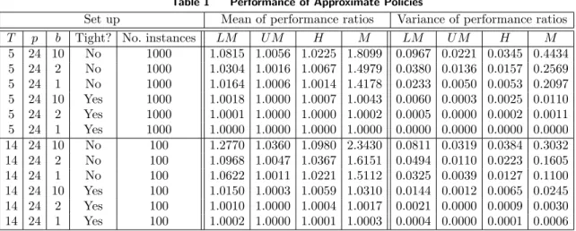
For each combination of the parameters, we generate a number of instances, i.e., binary proba-bility trees, for the demand structure based on the aforementioned distributional assumption (see Table 1). For each instance, we compute the optimal policyOP T using an exhaustive search. To facilitate computing the optimal policy we consider only integer-valued demand and allocation quantities. In addition toU M andLM, we have implemented two other policies. The first policy, a hybrid one denoted by H, is motivated by the results of Section 5. Since the outcomes of LM

andU M form bounds onOP T, our proposed policyH ensures that the waitlist in each period is the average of what it would have been underLM and U M. The second policy we consider is a myopic one, which minimizes the single-period cost given in (4), and we denote this policy byM. The outcome of our experiments show that that U M is the best-performing policy. In 6600 problem instances, the average performance ofU M is within 1.8% ofOP T compared to 35% for the naive myopic policy M. Under a range of problem configurations,U M’s performance is never

Table 1 Performance of Approximate Policies

Set up Mean of performance ratios Variance of performance ratios T p b Tight? No. instances LM U M H M LM U M H M

5 24 10 No 1000 1.0815 1.0056 1.0225 1.8099 0.0967 0.0221 0.0345 0.4434 5 24 2 No 1000 1.0304 1.0016 1.0067 1.4979 0.0380 0.0136 0.0157 0.2569 5 24 1 No 1000 1.0164 1.0006 1.0014 1.4178 0.0233 0.0050 0.0053 0.2097 5 24 10 Yes 1000 1.0018 1.0000 1.0007 1.0043 0.0060 0.0003 0.0025 0.0110 5 24 2 Yes 1000 1.0001 1.0000 1.0000 1.0002 0.0005 0.0000 0.0002 0.0011 5 24 1 Yes 1000 1.0000 1.0000 1.0000 1.0000 0.0000 0.0000 0.0000 0.0000 14 24 10 No 100 1.2770 1.0360 1.0980 2.3430 0.0811 0.0319 0.0384 0.3032 14 24 2 No 100 1.0968 1.0047 1.0367 1.6151 0.0494 0.0110 0.0223 0.1605 14 24 1 No 100 1.0622 1.0011 1.0221 1.5112 0.0325 0.0039 0.0127 0.1100 14 24 10 Yes 100 1.0150 1.0003 1.0059 1.0310 0.0144 0.0012 0.0065 0.0245 14 24 2 Yes 100 1.0010 1.0000 1.0004 1.0017 0.0021 0.0000 0.0009 0.0030 14 24 1 Yes 100 1.0002 1.0000 1.0001 1.0003 0.0004 0.0000 0.0001 0.0006

more than 3.6% away thanOP T, whereasM’s performance can be as much as 234% worse than that of OP T. The myopic policy does not perform well since it does not anticipate the long-term impact of a waitlist. Since the cost of postponing an elective patient by one period is small, a wait list is bad only if it is not resolved over many periods. Since the myopic policy sees only one period ahead, it severely over-allocates capacity to emergency surgeries. The performance statistics are summarized in Table 1, where the performance ratio is defined as the ratio of the total discounted cost under the scheduling policy in question to that under an optimal policy.

We see that U M consistently outperforms all other policies across a range of experimental settings. It exhibits both smaller average performance ratio with respect toOP T, as well as smaller variance for the performance ratios. By comparison, LM and H are within 4.8% and 2.4% of

OP T on average, respectively. Though they are slightly worse than U M, they seem to be much better than M. Recall that to derive U M and LM, we use the future cost of a limit policy as a substitute for the future cost of an optimal policy. The limit policy used to deriveU M allocates all available capacity in each period to emergency surgeries, whereas the limit policy used to derive

LM allocates all available capacity to elective cases. Since the cost of over-planning for emergency surgeries and making patients wait is typically much smaller than that of under-planning, the cost of the former limit policy is closer to optimal than that of the latter. Hence, as an approximation,

U M is expected to perform better than LM. Since U M is consistently better than LM, H is always worse thanU M because its performance lies between those of U M andLM.

We also find thatLM,U M, andH all perform much better than the myopic policyM, and thus the myopic policy may not be a good policy to use. All of our policies deteriorate in performance with longer horizons and higher waiting costs, although the degradation in performance for U M

is relatively small. All of the policies do better under capacity-tight instances because the decision space in these instances is more highly constrained. Hence the decisions undertaken by different policies are closer together and closer to those of OP T.

7.

Conclusion

In this paper we develop a capacity allocation model for allocation scheduling which explicitly considers multiple resources that are needed to serve two classes of patients with different wait-time sensitivities. Our model allows the demands, resource utilization and capacity availability to be random, non-stationary and time-correlated. We prove similar structural results for the optimal solutions as in the settings with i.i.d. demands. Our primary theoretical contribution is a method to obtain upper and lower bounds on the decisions of an optimal policy in each period. We also

develop several computationally-efficient policies which are shown to perform very well in our numerical experiments.

Our work is motivated by problems in health care service capacity management, in particular problems in surgical scheduling. Many important features in our model, such as dynamic and non-stationary environment and multi-resource constraints, are well recognized in the surgical-scheduling context (Cardoen et al. 2010, Moore et al. 2008, Dexter et al. 2005). Previous literature in this area usually assumes a simplified setup, such as i.i.d. demand structure and a single generic resource constraint. Our work is able to bring theory closer to practice by considering a much more general setup.

In our model, an elective patient does not receive an appointment at the time of joining the waitlist. This is not an uncommon practice in public health systems (such as Canada, UK and Australia). In the UK and Australia, waitlists are kept for elective patients, and they are considered useful in managing surgery schedules (Edwards 1997).

There are several ways to improve our model for practical application. First, it would be useful to consider patient heterogeneity in resource consumption within each patient type, i.e., emergency and elective. Second, we have assumed that patients only consume resources for one period, and it would be interesting to consider a model that allows patients to occupy some resource (e.g., beds) for multiple periods. Third, our model specifies how many elective patients to admit for the current period but not the timing or sequence of service. It would be interesting to develop a sequential decision model that jointly makes these decisions. All extensions above require substantially revised models and analysis, and we leave them for future research.

Acknowledgments

We thank the Editor, the Associate Editor and referees for constructive and positive feedback.

References

Ayvaz, N., W.T. Huh. 2010. Allocation of hospital capacity to multiple types of patients.Journal of Revenue & Pricing Management 9(5) 386–398.

Cardoen, B., E. Demeulemeester, J. Beli˙en. 2010. Operating room planning and scheduling: A literature review. European Journal of Operational Research 201(3) 921–932.

Chan, E., J. Muckstadt. 1999. Markov chain models for multi-echelon supply chains. Unpublished manuscript. Chan, E.W.M. 1999. Markov Chain Models for multi-echelon supply chains. Cornell University, August. Dexter, F., A. Macario, R.D. Traub, M. Hopwood, D.A. Lubarsky. 1999. An operating room scheduling

strategy to maximize the use of operating room block time: computer simulation of patient scheduling and survey of patients preferences for surgical waiting time. Anesthesia & Analgesia 89(1) 7–20. Dexter, F., E. Marcon, R.H. Epstein, J. Ledolter. 2005. Validation of statistical methods to compare

can-cellation rates on the day of surgery. Anesthesia & Analgesia 101(2) 465–473.

Dong, L., H.L. Lee. 2003. Optimal policies and approximations for a serial multiechelon inventory system with time-correlated demand. Operations Research 969–980.

Edwards, R.T. 1997. NHS waiting lists: towards the elusive solution. London: Office hof Health Economics. Gerchak, Y., D. Gupta, M. Henig. 1996. Reservation planning for elective surgery under uncertain demand

for emergency surgery. Management Science 42(3) 321–334.

Green, L.V., S. Savin, B. Wang. 2006. Managing patient service in a diagnostic medical facility. Operations Research 54(1) 11–25.

Gupta, D. 2007. Surgical suites’ operations management. Production and Operations Management 16(6) 689–700.

Iida, T., P. Zipkin. 2001. Approximate solutions of a dynamic forecast-inventory model. Working paper. Kuttenkuler, J. 2004. VCU neurosurgeon develops new device for performing deep brain surgery. Available

at:

http://www.news.vcu.edu/news/VCU neurosurgeon develops new device for performing deep brain. Levi, R., R. O. Roundy, D. B. Shmoys, V. A. Truong. 2008. Approximation algorithms for capacitated

Levi, Retsef, Martin P´al, Robin Roundy, David B. Shmoys. 2005. Approximation algorithms for stochastic inventory control models. Michael Jnger, Volker Kaibel, eds.,Integer Programming and Combinatorial Optimization,Lecture Notes in Computer Science, vol. 3509. Springer Berlin / Heidelberg, 306–320. Liu, N., S. Ziya, V.G. Kulkarni. 2010. Dynamic scheduling of outpatient appointments under patient no-shows

and cancellations. Manufacturing & Service Operations Management 12(2) 347–364.

Lu, X., J.S. Song, A. Regan. 2006. Inventory planning with forecast updates: approximate solutions and cost error bounds. Operations research 54(6) 1079.

Moore, I.C., D.P. Strum, L.G. Vargas, D.J. Thomson. 2008. Observations on surgical demand time series: detection and resolution of holiday variance. Anesthesiology109(3) 408–416.

¨

Ozer, Ozalp, G. Gallego. 2001. Integrating replenishment decisions with advance demand information. Managment Science 471344–1360.

Patrick, J., M.L. Puterman, M. Queyranne. 2008. Dynamic multi-priority patient scheduling for a diagnostic resource. Operations research56(6) 1507–1525.

Topkis, D.M. 1998. Supermodularity and complementarity. Princeton University Press, Princeton, NJ. Truong, V. A. 2011. The pediatric vaccine stockpiling problem. Under review.

Ward, A.R., P.W. Glynn. 2003. A diffusion approximation for a markovian queue with reneging. Queueing Systems 43(1) 103–128.

Online Appendix

Lemma EC.1. IfV(z)is a convex function in z andais a positive constant, then V(x−ay)is submodular inx andy.

Proof: Take arbitrary x1> x2. Since V(·) is convex, its marginal increment is increasing and

thereforeV(x1−ay)−V(x2−ay) decreases iny, which completes the proof.!.

Proof of Lemma 1:The joint convexity ofL(qt, Bt, Ft) inBtandqtis evident from (4). It is easy

to see the submodularity of the first term in L(qt, Bt, Ft). Since the second term of this function

only involvesqt, it is also submodular inqt andBt. These prove the desired results with respect to

Bt andqt.

Now define ˜L(zt, Bt, Ft) =L(Bt−zt, Bt, Ft), where zt representsBt−qt. Then, from (4),

˜

L(zt, Bt, Ft) = (b+cE[ξt|Ft])zt+pτE(At2et+At1(Bt−zt)−ut)+ ,

which can also be shown to be convex and submodular in (zt, Bt) by Lemma EC.1.!.

Proof of Lemma 2: Substituting rt= (ut−At1qt)/At2, the problem of minimizing (7) with

respect toqt is equivalent to minimizing the following expression with respect tort:

(b+cE[ξt|Ft]) At2 At1 rt+pAt2Eet[et−rt|Ft] + , (EC.1)

where max{0,(ut−At1Bt)/At2}≤rt≤ut/At2. Without the constraint onrt, this is the newsvendor

problem with the uncertain demandet, the purchase cost (b+cE[ξt|Ft])A_At2

t1, and the backlog penalty

pAt2. Thus the optimal value of rt for this unconstrained newsvendor problem is rtnv as noted

above. Considering the bounds onrt and the convexity of (EC.1) with respect tort, we obtain the

desired results. !.

Proof of Lemma 3:We prove these results by induction. It is easy to see that the terminal cost

VT+1(BT+1, FT+1) =vBT+1 is a linear and increasing function of the final backlogBT+1.

Now, suppose that the statements are true for t+ 1. We first prove statement (a) for t. Since

L(qt, Bt, Ft) is jointly convex in (qt, Bt) (by Lemma 1) andVt+1is jointly convex (induction

hypoth-esis), it follows from (6) thatGtis jointly convex in (qt, Bt). Also, the submodularity ofGt follows

from the submodularity of L(Lemma 1) and the joint convexity of Vt+1 in Bt and qt (induction

hypothesis and Lemma EC.1 in the Appendix). This completes the proof of (a) fort.

Statement (b) fortfollows directly sinceL(qt, Bt, Ft) is increasing inBtfrom (4), and the second

term in the right-side of (6) is increasing inBt from the induction hypothesis.

Now we consider statement (c) fort. SinceG(qt, Bt, Ft) is jointly convex in (qt, Bt) from statement

(a) and the feasible region of the minimization operator in (5) is convex, we obtain thatVt(Bt, Ft)

is also convex inBt. Finally, to showVt(Bt, Ft) increases inBt, consider the case whereBtincreases

to Bt+δ for some δ>0. It is easy to see that Gt(q, Bt, Ft)≤Gt(q, Bt+δ, Ft) for any 0≤q≤Bt

(from statement (b)). Furthermore, we can show that Gt(Bt, Bt, Ft)≤Gt(q, Bt+δ, Ft) for any

Bt< q≤Bt+δsince we obtain from (6) that

Gt(Bt, Bt, Ft) =L(Bt, Bt, Ft) +αE ! Vt+1((1−ξt)(Bt−Bt) +dt+1, Ft+1) " "Ft # ≤L(q, Bt+δ, Ft) +αE ! Vt+1((1−ξt)(Bt+δ−q) +dt+1, Ft+1) " "Ft # = Gt(q, Bt+δ, Ft) ,

where the inequality follows from the definition of Lin (4) and the induction hypothesis onVt+1.

Therefore, it follows that min0≤qt≤BtGt(qt, Bt, Ft) ≤ min0≤qt≤Bt+δGt(qt, Bt+δ, Ft), implying by

the definition of Vt in (5) thatVt(Bt, Ft) increases inBt.

Now we consider (d). From (a), Gt is jointly convex and submodular in (qt, Bt). Rewrite