Imperial College London
Department of Computing
Diagnosing, Predicting and Managing
Application Performance in Virtualised
Multi-Tenant Clouds
Xi Chen
Submitted in part fulfilment of the requirements for the degree of Doctor of Philosophy in Computing of Imperial College London
and the Diploma of Imperial College London July 2016
Abstract
As the computing industry enters the cloud era, multicore architectures and virtualisation technologies are replacing traditional IT infrastructures for several reasons including reduced infrastructure costs, lower energy consumption and ease of management. Cloud-based software systems are expected to deliver reliable performance under dynamic workloads while efficiently allocating resources. However, with the increasing diversity and sophistication of the environ-ment, managing performance of applications in such environments becomes difficult.
The primary goal of this thesis is to gain insight into performance issues of applications run-ning in clouds. This is achieved by a number of innovations with respect to the monitoring, modelling and managing of virtualised computing systems: (i) Monitoring – we develop a mon-itoring and resource control platform that, unlike early cloud benchmarking systems, enables service level objectives (SLOs) to be expressed graphically as Performance Trees; these source both live and historical data. (ii) Modelling – we develop stochastic models based on Queue-ing Networks and Markov chains for predictQueue-ing the performance of applications in multicore virtualised computing systems. The key feature of our techniques is their ability to charac-terise performance bottlenecks effectively by modelling both the hypervisor and the hardware. (iii) Managing – through the integration of our benchmarking and modelling techniques with a novel interference-aware prediction model, adaptive on-line reconfiguration and resource control in virtualised environments become lightweight target-specific operations that do not require sophisticated pre-training or micro-benchmarking.
The validation results show that our models are able to predict the expected scalability be-haviour of CPU/network intensive applications running on virtualised multicore environments with relative errors of between 8 and 26%. We also show that our performance interference prediction model can capture a broad range of workloads efficiently, achieving an average error of 9% across different applications and setups. We implement this model in a private cloud de-ployment in our department, and we evaluate it using both synthetic benchmarks and real user applications. We also explore the applicability of our model to both hypervisor reconfiguration and resource scheduling. The hypervisor reconfiguration can improve network throughput by up to 30% while the interference-aware scheduler improves application performance by up to 10% compared to the default CloudStack scheduler.
Acknowledgements
I would like to thank the following people:
• My supervisor, Prof William Knottenbelt, who guided me tirelessly through my PhD. He’s a brilliant researcher and advisor who was always ready to help, encourage and push ideas one level further, and share his experience and insight about any problem. His commitment to excellence is inspiring; his belief in his students is motivating; his enthusiasm for research problems is catching. I have been very fortunate to work with him and infected by his knowledge, vision, passion, optimism and inspiration everyday. • The head of the Department of Computing, Prof Susan Eisenbach, for her support and
the financial assistance, the departmental international student scholarship.
• Dr Felipe Franciosi, for his efforts in improving the experiments and ideas, providing insightful knowledge, and encouragement and help in broad areas.
• The DoC Computing Support Group (CSG) for their countless and prompt help, and extremely awesome hand-on knowledge, and incredible problem solving techniques, and their kind, patiences, understanding and endlessly support. In particular: I would like to thank Mr Duncan White, Dr Lloyd Kamara and Thomas Joseph for helping me with the many environmental setups, system configurations and countless difficult problems, and many evenings that they had to work late because of these.
• My collaborators, Chin Pang Ho from Computational Optimisation Group for his great input on the mathematical analysis and many other math problems, and Lukas Rup-precht from LSDS group for his broad knowledge and experience on experiment design, distributed systems and many valuable discussions. The work in this dissertation is the result of collaboration with many other people, more broadly numerous people, Prof Pe-ter Harrison, Giuliano Casale, Tony Field, Rasha Osman, Gareth Jones in AESOP group contributed to the development and refinement of the ideas in this thesis.
• Dr Amani El-Kholy for her endless love, trust, and support for the last 6 years.
• My examiners, Prof Kin Leung and Dr Andrew Rice, for kindly agreeing to serve as internal and external examiners for my viva. Their careful review and their insightful
• And last but not least my family and friends, for their infinite love and perpetual support no matter what I do or what I chose, especially during the hard times that happened 8 hours time difference away from home.
Dedication
To my family
Copyright Declaration
© The copyright of this thesis rests with the author and is made available under a Creative Commons Attribution Non-Commercial No Derivatives licence. Researchers are free to copy, distribute or transmit the thesis on the condition that they attribute it, that they do not use it for commercial purposes and that they do not alter, transform or build upon it. For any reuse or redistribution, researchers must make clear to others the licence terms of this work.
Contents
Abstract i
Acknowledgements iii
1 Introduction 1
1.1 Motivation . . . 1
1.2 Objectives and Aims . . . 3
1.3 Contributions . . . 5
1.3.1 A Performance Tree-based Monitoring Platform for Clouds . . . 5
1.3.2 Investigating and Modelling the Performance of Web Applications in Mul-ticore Virtualised Environments . . . 7
1.3.3 Diagnosing and Managing Performance Interference in Multi-Tenant Clouds 8 1.4 Statement of Originality and Publications . . . 8
1.5 Thesis Roadmap . . . 9
2 Background 10 2.1 Introduction . . . 10
2.2 Cloud Computing . . . 10
2.3 Characterising Virtualised Multicore Scalability . . . 11 ix
2.3.1 Multicore and Scalability . . . 12
2.3.2 Linux Kernel Internals and Imbalance of Cores . . . 13
2.3.3 Virtualisation and Hypervisor Overhead . . . 13
2.4 Characterising Performance Interference Caused by Virtualisation . . . 14
2.4.1 Xen and Paravirtualisation . . . 15
2.4.2 CPU Scheduler . . . 17
2.4.3 Disk I/O . . . 19
2.4.4 Grant Table . . . 19
2.4.5 Network I/O . . . 20
2.5 Stochastic Modelling . . . 21
2.5.1 Discrete-time Markov Chains . . . 21
2.5.2 Transition Matrix and State Transition Diagram . . . 23
2.5.3 State Transition Probability Distribution . . . 23
2.5.4 Steady State and Stationary Distribution . . . 26
2.6 Queueing Theory . . . 27
2.6.1 Important Performance Measures . . . 28
2.6.2 Processor-sharing Queueing Models . . . 29
2.6.3 BCMP Network . . . 30
2.7 Performance Trees . . . 32
2.8 Related Research . . . 34
2.8.1 Cloud Benchmarking Systems . . . 34
2.8.2 Performance Modelling of Web Applications in Virtualised Environments 35 2.8.3 Performance Interference Modelling in Multi-Tenant Clouds . . . 38
CONTENTS xi
3 A Performance Tree-based Monitoring Platform for Clouds 42
3.1 Introduction . . . 42
3.2 The Design of a Performance Tree-based Monitoring Platform . . . 43
3.2.1 System Requirements . . . 43
3.2.2 System Architecture . . . 44
3.3 The Myth of Monitoring in Clouds . . . 46
3.3.1 Measuring without Virtualisation . . . 46
3.3.2 Measuring with Virtualisation . . . 48
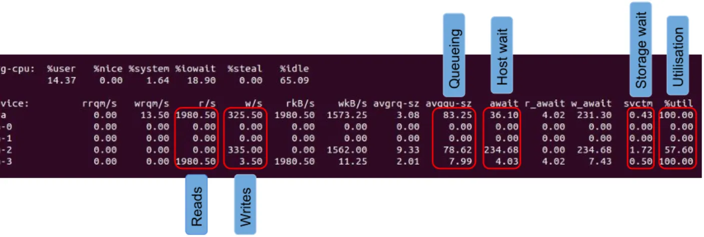
3.3.3 An Example of Measuring the Actual I/O Queue Size . . . 52
3.4 GUI and Demo in Action . . . 55
3.5 Summary . . . 56
4 Predicting the Performance of Applications in Multicore Virtualised Envi-ronments 57 4.1 Introduction . . . 57 4.2 Benchmarking . . . 59 4.3 Proposed Model . . . 63 4.3.1 Model Specification . . . 63 4.3.2 CPU 0 . . . 65
4.3.3 Two-class Markov Chain and its Stationary Distribution of CPU 0 . . . . 65
4.3.4 Average Sojourn Time of CPU 0 . . . 68
4.3.5 Average Service Time and Utilisation of CPU 0 . . . 70
4.3.7 Combined Model . . . 73
4.3.8 Validation . . . 74
4.4 Scalability and Model Enhancement . . . 75
4.4.1 Scalability Enhancement . . . 76
4.4.2 Model Enhancement . . . 76
4.4.3 Prediction with Previous Parameters . . . 77
4.4.4 Prediction validation for Type I hypervisor – Xen . . . 80
4.4.5 Model Limitations . . . 80
4.5 Summary . . . 80
5 Diagnosing and Managing Performance Interference in Multi-Tenant Clouds 82 5.1 Introduction . . . 82
5.2 Characterising Performance Interference . . . 85
5.2.1 Recapping Xen Virtualisation Background . . . 85
5.2.2 Measuring the Effect of Performance Interference . . . 86
5.3 System Design . . . 89
5.3.1 Predicting Performance Interference . . . 91
5.3.2 CPU workloads . . . 92
5.3.3 I/O workloads . . . 93
5.3.4 Virtualisation Slowdown Factor . . . 95
5.4 Interference Conflict Handing . . . 96
5.4.1 Dynamic Interference Scheduling . . . 97
5.5 Evaluation . . . 99
5.5.1 Experimental Setup . . . 99
5.5.2 CPU, Disk, and Network Intensive Workloads . . . 100
5.5.3 Mixed Workload . . . 101
5.5.4 MapReduce Workload . . . 102
5.5.5 Interference-aware Scheduling . . . 104
5.5.6 Adaptive Control Domain . . . 107
5.6 Summary . . . 108
6 Conclusion 110 6.1 Summary of Achievements . . . 111
6.2 Future Work . . . 113
A Xen Validation Results 115
Bibliography 117
List of Tables
4.1 Summary of the key parameters in the multicore performance prediction model . 74 4.2 Likelihood estimation of the mean service of classb job . . . 74
4.3 Relative errors between model and measurements (%) . . . 79
5.1 Benchmarking configuration of interference prediction . . . 86 5.2 Specifications for interference-aware scheduler experimental environment . . . . 104 5.3 Related work of virtualisation interference prediction . . . 108
List of Figures
1.1 The decision making hierarchy . . . 4
1.2 The overview of this thesis . . . 6
2.1 Context switching inside a multicore server . . . 12
2.2 A brief history of virtualisation . . . 15
2.3 Xen hypervisor architecture with guest virtual machines . . . 17
2.4 A state transition diagram example . . . 24
2.5 An example of Performance Tree query . . . 32
3.1 An example of Performance Tree-based SLO evaluation . . . 44
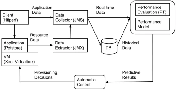
3.2 System architecture . . . 45
3.3 The screenshot of iostat running fio benchmark tests . . . 48
3.4 The path of an application issuing requests to disks without virtualisation . . . 52
3.5 The sequence diagram of an application issuing requests to disks . . . 53
3.6 The path of an application issuing requests to disks with virtualisation . . . 53
3.7 The sequence diagram of an application issuing requests to disks with virtualisation 54 3.8 Performance Tree evaluation GUI . . . 56
4.1 Testbed Infrastructures for Type-1 Hypervisor (left) and Type-2 Hypervisor (right) 60 xvii
4.3 Response time and throughput of 1 to 8 core VMs running web application . . . 62
4.4 Modelling a multicore server using a network of queues . . . 63
4.5 State transition diagram of CPU 0 . . . 66
4.6 Comparing numerical and analytical solution E(K) . . . 68
4.7 Response time validation of 1 to 8 core with 1 NIC . . . 75
4.8 Revalidation of response time of 1 to 8 core with multiple number of NICs . . . 78
5.1 The load average (utilisation) example of the VM running sysbench experiment 87 5.2 Co-resident VM performance measurements for CPU, disk and network intensive workloads . . . 88
5.3 CloudScope system architecture . . . 90
5.4 State transition diagrams for CPU, disk and network insensitive workloads . . . 92
5.5 Interference prediction model validation for CPU, disk and network intensive workloads. . . 100
5.6 Interference prediction and model validation of mixed workloads . . . 102
5.7 Interference prediction model validation for different Hadoop Yarn workloads with different numbers of mappers and reducers . . . 103
5.8 Histograms of the performance improvement of the CloudScope interference-aware scheduler over the CloudStack scheduler . . . 105
5.9 CDF plots for the job completion times of different tasks under CloudScope compared to CloudStack . . . 106
5.10 CloudScope scheduling results compared to the default CloudStack scheduler . . 108
5.11 CloudScope self-adaptive Dom0 with different vCPU weights . . . 108 xviii
A.1 Validation of response time of 1 to 8 core with multiple number of NICs on Xen hypervisor . . . 116
Chapter 1
Introduction
1.1
Motivation
Cloud computing refers to both the applications delivered as services over the Internet and the hardware and software in the data centres that provide those services [AFG+10]. The demand
for cloud computing has continuously been increasing during recent years. Millions of servers are hosted and utilised in cloud data centres every day and many organisations deploy their own virtualised computing infrastructure [OWZS13, MYM+11]. Virtualisation is the technol-ogy that enables the cloud to multiplex different workloads and to achieve elasticity and the illusion of infinite resources. By 2016, it is anticipated that more than 80% of enterprise work-loads will be using IaaS (Infrastructure as a Service) clouds [Col16], whether these are public, private and hybrid. Virtualisation and multicore technologies both enable and further en-courage this trend, increasing platform utilisation via consolidating multiple application work-loads [RTG+12, ABK+14]. This computing paradigm provides improved performance, reduced application design and deployment complexity, elastic handling of dynamic workloads, and lower power consumption compared to traditional IT infrastructures [NSG+13, GNS11a, GLKS11]. Efficient application management over cloud-scale computing clusters is critical for both cloud providers and end users in terms of resource utilisation, application performance and system throughput. Strategies for resource allocation in different applications and virtual resource
solidation increasingly depend on understanding the relationship between the required perfor-mance of applications and system resources [SSGW11, TZP+16]. To increase resource efficiency
and lower operating costs, cloud providers resort to consolidating virtual instances, i.e. pack-ing multiple applications into one physical machine [RTG+12]. Analysis performed by Google
shows that up to 19 distinct applications and components are co-deployed on a single multicore node in their data centres [KMHK12]. Understanding the performance of consolidated appli-cations is important for cloud providers to maximise resource utilisation and augment system throughput while maintaining individual application performance targets. Satisfying perfor-mance within a certain level of Service Level Objectives (SLOs) is also important to end users because they are keen to know their applications are provisioned with sufficient resources to cope with varying workloads. For instance, local web server infrastructure may not be provi-sioned for high-volume requests, but it may be feasible to rent capacity from the cloud for the duration of the increasing volume [LZK+11, ALW15].
Further, performance management in clouds is becoming even more challenging with grow-ing cluster sizes and more complex workloads with diverse characteristics. Major cloud ser-vice vendors not only provide a variety of VMs that offer different levels of compute power (including GPU), memory, storage, and networking, but also a broad selection of services, e.g. web servers, databases, network-based storage or in-network services such as load bal-ancers [ABK+14, TBO+13]. A growing number of users from different organisations submit
jobs to these clouds every day. Amazon EC2 alone has grown from 9 million to 28 million public IP addresses in the past two years [Var16]. The submitted jobs are diverse in nature, with a variety of characteristics regarding the amount of requests, the complexity of processing, the degree of parallelism, and the resource requirements.
Beside the fact that applications running in clouds exhibit a high degree of diversity, they also remain highly variable in performance. Whereas efforts have improved both the raw performance and performance isolation of VMs, the additional virtualisation layer makes it hard to achieve bare metal performance in many cases. Multicore platforms and their current hypervisor-level resource isolation management continues to be challenged in their ability to meet the performance of multiple consolidated workloads [ZTH+13]. This is due to the fact
1.2. Objectives and Aims 3
that an application’s performance is determined not only by its use of CPU and memory capacities, which can be carefully allocated and partitioned [BDF+03, HKZ+11], but also its
use of other shared resources, which are not easy to control in an isolated fashion, e.g. I/O resources [TGS14]. As a result, cloud applications and appliance throughput varies by up to a factor of 5 times in data centres due to resource contention [BCKR11]. Therefore, developers and cloud managers require techniques to help them measure their applications executed in such environments. Furthermore, they need to be able to diagnose and manage application performance issues.
In summary, resource management in hypervisors or cloud environments must manage in-dividual elastic applications along multiple resource dimensions while dealing with dynamic workloads, and they must do so in a way that considers the runtime resource costs of meeting the application requirements while understanding the performance implications caused by other co-resident applications due to indirect resource dependencies.
1.2
Objectives and Aims
Our primary goal is to develop performance analysis techniques and tools that can help end users and cloud providers to manage application performance efficiently. We tackle this goal in the context of the decision making hierarchy shown in Figure 1.1. At the bottom level, we develop monitoring and resource control tools to help describe ‘what is going on?’ in the system. Next, we predict ‘what is going to happen if something changes?’ using performance models. Finally, at the highest level, we prescribe the corresponding performance management actions to answer ‘what value-adding decision can we make?’ for improved performance.
The primary research hypothesis that emerges from the above is: Within the context of virtualised environments, and with appropriate tool and user interface support, performance modelling can help to diagnose system bottlenecks and to improve resource allocation decision in a way that increases horizontal scalability and lowers interference between co-resident VMs. Our hypothesis has a broad scope and the related work, such as performance benchmarking
Description (monitoring) Prediction (modelling) Prescription (managing)
What value-adding decision can we make?
What is going to happen if something changes?
What is going on?
Figure 1.1: The decision making hierarchy
systems, performance modelling and resource management techniques, has been intensively studied. Yahoo!’s YCSB [CST+10], MalStone [BGL+10], and COSBench [ZCW+13] are pro-posed to create standard benchmarking frameworks for evaluating the performance of differ-ent cloud systems, e.g. data processing systems, web services, cloud object storage etc. At the same time, researchers have developed specialised prediction models [BGHK13, CGPS13, BM13, DK13, CH11, NKG10, NBKR13, CKK11] to capture and predict performance under dif-ferent workloads. These systems and techniques cope with certain aspects of the performance management problem in cloud environments; however, they also come with several drawbacks. We are going to present the objectives of this dissertation with the observation of current systems and research. In this context the objectives of this thesis are:
1. To support flexible and intuitive performance queries: Many benchmarking frame-works provide limited support for flexible and intuitive performance queries. Some of them provide users with a query interface or a textual query language [GBK14], leading to management difficulty for complex performance evaluation and decision making. We seek to design an intuitive graphical specification of complex performance queries that can reason about a broader range of concepts related to application SLOs than current alternatives [DHK04, CCD+01].
2. To provide an automatic resource control: If an application does not fulfil the performance requirements, the user must either manually decide on the scaling options
1.3. Contributions 5
and new instance types, or else write a new module in the system calling corresponding cloud APIs to do so [BCKR11, FSYM13]. Efficient performance management should be enhanced with self-managing capabilities, including self-configuration and self-scaling once the performance is violated.
3. To provide lightweight and detailed models for targeted prediction: It is both expensive and unwieldy to compose a prediction model based on comprehensive micro-benchmarks or on-line training [DK13, CH11, NKG10, RKG+13, CSG13, KEY13, ZT12, YHJ+10]. Current clouds require prediction to be general and efficient enough for complex environments where applications change frequently. Apart from being lightweight, low-level resource behaviour such as the utilisation of different CPU cores needs to be captured to support fine-grained and target-specific resource allocation.
4. To investigate system and VM control strategies for better performance: Based on the resource demand and performance prediction, successful management needs to be able to not only add or remove servers [SSGW11, ZTH+13, NSG+13], but also to seek the best configuration of the underlying servers and the hypervisor in order to serve the guest VM applications in a more efficient way.
1.3
Contributions
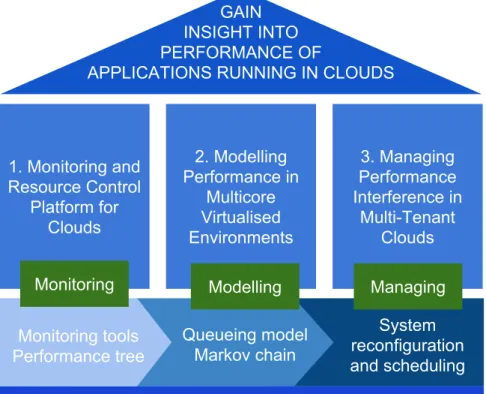
As shown in Figure 1.2, this thesis presents a number of innovations with respect to monitoring, modelling and managing the performance of applications in clouds. We outline the contributions made in this dissertation and several key advantages over current techniques and methods.
1.3.1
A Performance Tree-based Monitoring Platform for Clouds
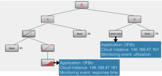
We implement a real time performance monitoring, evaluation and resource control platform that reflects well the characteristics of contemporary cloud computing (e.g. extensible, user-defined, scalable). The front-end allows for the graphical specification of SLOs using
Perfor-GAIN INSIGHT INTO PERFORMANCE OF
APPLICATIONS RUNNING IN CLOUDS
1. Monitoring and Resource Control Platform for Clouds 2. Modelling Performance in Multicore Virtualised Environments 3. Managing Performance Interference in Multi-Tenant Clouds
Monitoring Modelling Managing
Monitoring tools Performance tree Queueing model Markov chain System reconfiguration and scheduling Cloud Systems, hypervisor, applications
1.3. Contributions 7
mance Trees (PTs), while violated SLOs trigger mitigating resource control actions. SLOs can be specified over both live and historical data, and can be sourced from multiple applications running on multiple clouds. We clarify that our contribution is not in the development of the formalism (which is defined in [SBK06, KDS09]), nor in the Performance Tree evaluation environment [BDK+08]. Rather it concerns the application of Performance Trees to cloud
envi-ronments. Specifically, we demonstrate how our system is capable of monitoring and evaluating the application performance, and ensuring the SLOs of a target cloud application are achieved by resource auto-scaling. Our system is amenable to multi-tenancy and multi-cloud environ-ments, allowing applications to meet their SLOs in an efficient and responsive fashion through automatic resource control.
1.3.2
Investigating and Modelling the Performance of Web
Appli-cations in Multicore Virtualised Environments
As the computing industry enters the Cloud era, multicore architectures and virtualisation technologies are replacing traditional IT infrastructures. However, the complex relationship between applications and system resources in multicore virtualised environments is not well understood. Workloads such as web services and on-line financial applications have the re-quirement of high performance but benchmark analysis suggests that these applications do not optimally benefit from a higher number of cores [HBB12, HKAC13]. We begin by bench-marking a real web application, noting the systematic imbalance that arises with respect to per-core workload. Having identified the reason for this phenomenon, we propose a queueing model which, when appropriately parametrised, reflects the trend in our benchmark results for up to 8 cores. Key to our approach is providing a fine-grained model which incorporates the idiosyncrasies of the operating system and the multiple CPU cores. Analysis of the model suggests a straightforward way to mitigate the observed bottleneck, which can be practically realised by the deployment of multiple virtual NICs within the VM. It is interesting to add virtual hardware to the existing VM to improve performance (at no actual hardware cost). We validate the model against direct measurements based on a real system. The validation results
show that the model is able to predict the expected performance across different number of cores and virtual NICs with relative errors ranging between 8 and 26%.
1.3.3
Diagnosing and Managing Performance Interference in
Multi-Tenant Clouds
Virtual machine consolidation is attractive in cloud computing platforms for several reasons including reduced infrastructure costs, lower energy consumption and ease of management. However, the interference between co-resident workloads caused by virtualisation can violate the SLOs that the cloud platform guarantees. Existing solutions to minimise interference be-tween VMs are mostly based on comprehensive micro-benchmarks or online training which makes them computationally intensive. We develop CloudScope, a system for diagnosing inter-ference for multi-tenant cloud systems in a lightweight way. CloudScope employs a discrete-time Markov chain model for the online prediction of performance interference of co-resident VMs. It uses the results to (re)assign VMs to physical machines and to optimise the hypervisor configuration, e.g. the CPU share it can use, for different workloads. We implement Cloud-Scope on top of the Xen hypervisor and conduct experiments using a set of CPU, disk, and network-intensive workloads and a real system (MapReduce). Our results show that Cloud-Scope interference prediction achieves an average error of 9%. The interference-aware scheduler improves VM performance by up to 10% compared to the default scheduler. In addition, the hypervisor reconfiguration can improve network throughput by up to 30%.
1.4
Statement of Originality and Publications
I declare that this thesis was composed by myself, and that the work that it presents is my own except where otherwise stated.
1.5. Thesis Roadmap 9
• 6th ACM/SPEC International Conference on Performance Engineering(ICPE 2015) [CK15] presents a Performance Tree-based monitoring and resource control platform for clouds. The work presented in Chapter 3 is based on this paper.
• 5th ACM/SPEC International Conference on Performance Engineering(ICPE 2014) [CHO+14] presents a performance model for web applications deployed in multicore
virtualised environments. The work presented in Chapter 4 is based on this paper. • 23rd International Symposium on Modeling, Analysis and Simulation of
Com-puter and Telecommunications Systems (MASCOTS 2015) [CRO+15] presents a
comprehensive system, CloudScope, to predict resource interference in virtualised envi-ronments, and use the prediction to enhance the operation of cloud platforms. The work presented in Chapter 5 is based on this paper.
1.5
Thesis Roadmap
The reminder of this dissertation is structured as follows. We explore the background and the related work in Chapter 2. In Chapter 3, we introduce a Performance Tree-based monitoring and resource control platform. In Chapter 4, we present a model that captures the performance of web applications in multicore virtualised environments. In Chapter 5, we present CloudScope, a system that diagnoses the bottlenecks of co-resident VMs and mitigates their interference based on a lightweight prediction model. Chapter 6 concludes this dissertation with a summary of our achievements and a discussion of future work.
Background
2.1
Introduction
This chapter presents background related to the understanding and modelling of the systems that we focus on. We begin by giving an overview of cloud computing, followed by a description of two major enabling technologies heavily used in clouds: multicore architectures and virtual-isation. We highlight the most important properties of the workloads and systems with a view to incorporate them into an analytical model. We then present an overview of Markov chains and Queueing theory, which are the key techniques we use for performance modelling. Next, we briefly recap how Performance Trees can be utilised for graphical performance queries and eval-uation. We conclude by reviewing the related scientific literature covering cloud benchmarking systems, performance modelling for virtualised multicore systems and performance interference prediction and management in multi-tenant cloud environments.
2.2
Cloud Computing
Cloud computing platforms are becoming increasingly popular for hosting enterprise applica-tions due to their ability to support dynamic provisioning of virtualised resources. Multicore
2.3. Characterising Virtualised Multicore Scalability 11
systems are widespread in all types of computing systems, from embedded to high-performance servers, which are widely provided in these public cloud platforms. More than 80% of mail services (e.g. Gmail, or Yahoo!), personal data storage (e.g. Dropbox), on-line delivery (e.g. Domino pizza), video streaming services (e.g. Netflix) and many other services are supported by cloud-based web applications [CDM+12, ABK+14, ALW15, PLH+15]. Flexibility, high
scal-ability and low-cost delivery of services are key drivers of operational efficiency in many organi-sations. However, the sophistication of the deployed hardware and software architectures makes the performance studies of such applications very complex [CGPS13]. Often, enterprise appli-cations experience dynamic workloads and unpredictable performance [ABG15, ZCM11]. As a result, provisioning appropriate and budget-efficient resource capacity for these applications remains an important and challenging problem.
Another reason for variable performance and a major feature of cloud infrastructure, is the fact that the underlying physical infrastructure is shared by multiple virtual instances. Although modern virtualisation technology provides performance isolation to a certain extent, the com-bined effects from concurrent applications, when deployed on shared physical resources, are difficult to predict, and so it is problematic to achieve application SLOs. For example, a MapReduce cloud service has to deal with the interference deriving from contention in numer-ous hardware components, including CPU, memory, I/O bandwidth, the hypervisor, and their joint effects [BRX13, DK13, WZY+13]. Our goal is to build on the capability of performance
modelling to provide significant gains in automatic system management, in particular (a) im-proving the horizontal scalability of a multicore virtualised system and (b) diminishing the interference between co-resident VMs. We discuss the key aspects of each of these objectives in the subsections below.
2.3
Characterising Virtualised Multicore Scalability
Here we present the background related to capturing the behaviour under scaling of CPU and network intensive workloads (e.g. web applications) running on multicore virtualised platforms.
We start by briefly introducing multicore architectures; then we explain the basic steps involved in receiving/transmitting traffic from/to the network and finally discuss the overhead introduced by virtualisation.
2.3.1
Multicore and Scalability
To exploit the benefits of a multicore architecture, applications need to be parallelised [PBYC13, VF07]. Parallelism is mainly used by operating systems at the process level to provide mul-titasking [GK06]. We assume that the following two factors are inherent to web applications which scale with the number of cores: (1) the workload of a web application typically involves multiple concurrent client requests on the server and hence is easily parallelisable; (2) they exploit the multithreading and asynchronous request services provided by modern web servers (such as Nginx). Each request is usually processed in a separate thread and threads can run simultaneously on different CPUs. As a result, modern web servers can efficiently utilise mul-tiple CPU cores. However, scalability of web servers is not linear in practice as other factors, such as synchronisation, sequential workflows, communication overhead, cache pollution, and call-stack depth [NBKR13, VF07, CSA+14, JJ09] limit the performance.
0 1 n-1
2.3. Characterising Virtualised Multicore Scalability 13
2.3.2
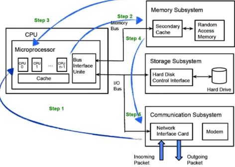
Linux Kernel Internals and Imbalance of Cores
Modern computer architectures are interrupt-driven. If a device, such as a network interface card (NIC) or a hard disk, requires CPU cycles to support an I/O operation, it triggers an inter-rupt which calls a corresponding handler function [TB14]. As we investigate web applications, we focus oninterrupts generated by NICs. When packets from the network arrive, the NIC places these in an internal packet queue and generates an interrupt to notify the CPU to process the packet. By default, an interrupt is handled by a single CPU (usually CPU 0). Figure 2.1 illustrates the process of passing a packet from the network to the application and sending a response back to the network (steps 1 to 5). The NIC driver copies the packet to memory and generates a hardware interrupt to signal the kernel that a new packet is readable (step 1). A previously registered interrupt handler is called which generates a software interrupt to push the packet down to the appropriate protocol stack layer or application (step 2) [WCB07]. By default, a NIC software interrupt is handled by CPU 0 (core 0) which induces a non-negligible load and, as processing rates increase, creates a major bottleneck for web applications (interrupt storm) [VF07]. Modern NICs can support multiple packet queues. The driver for these NICs typically provides a kernel module parameter to configure multiple queues [PJD04, JJ09] and assign an interrupt to the corresponding CPU (step 3). The signalling path for PCI (Peripheral Component Interconnect) devices uses message signalled interrupts (MSI-X) that can route each interrupt to a particular CPU [PJD04, HKAC13] (step 4). The NIC triggers an associated interrupt to notify a CPU when new packets arrive or depart on the given queue (step 5).
2.3.3
Virtualisation and Hypervisor Overhead
In the context of modelling the performance of web applications running in virtualised envi-ronments, the relationship between application performance and virtualisation overhead must be taken into account. The virtualisation overhead greatly depends on the different requirements of the guest workloads on the host hardware. With technologies like
VT-x/AMD-V1 and nested paging2, the CPU-intensive guest code can run very close to 100% native speed whereas I/O can take considerably longer due to virtualisation [GCGV06]. For ex-ample, Barham et al. [BDF+03] show that the CPU-intensive SPECweb99 benchmark and the
I/O-intensive Open Source Database Benchmark suite (OSDB) exhibit very different behaviour in native Linux and XenoLinux (based on the Xen hypervisor). PostgreSQL in OSDB places considerable load on the disk resulting in multiple domain transitions which are reflected in the substantial virtualisation overhead. SPECweb99, on the other hand, does not require these transitions and hence obtain very nearly the same performance as a bare machine [BDF+03].
2.4
Characterising Performance Interference Caused by
Virtualisation
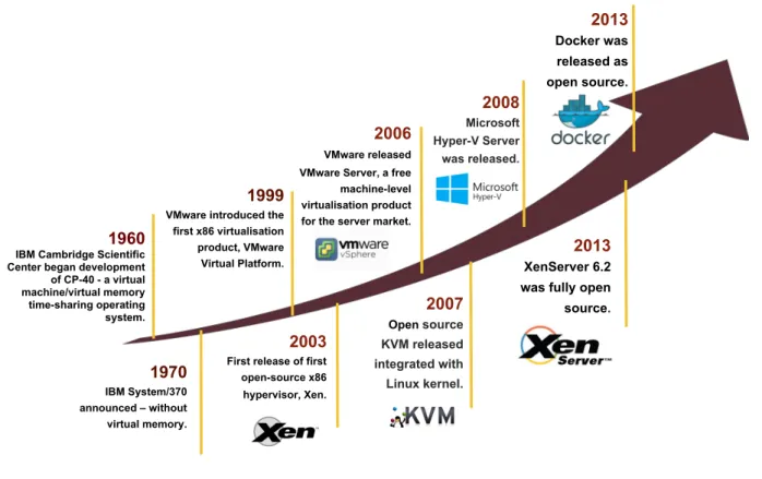
The IT industry’s focus on virtualisation technology has increased considerably in the past few years. In this section, we will recap the history of virtualisation and the key technologies behind it. Figure 2.2 shows a brief overview of virtualisation technology over time. The concept of virtualisation is generally believed to have its origins in the mainframe days back in the late 1960s and early 1970s when IBM invested a lot of time and efforts in developing robust time-sharing solutions3, e.g. the IBM CP-40 and the IBM System/370. Time-sharing refers to
the shared usage of computer resources among a large group of users, aiming to increase the efficiency of both the user and the expensive compute resources they share. The best way to improve resource utilisation, and at the same time simplify data centre management, is through this time-sharing idea – virtualisation. Virtualisation is defined as enabling multiple operating systems to run on a single host computer, and the essential component in the virtualisation stack is the hypervisor. Hypervisors are commonly classified as one of these two types:
1“Hardware-assisted virtualization,” in Wikipedia: The Free Encyclopedia; available from https://en.
wikipedia.org/wiki/Hardware-assisted_virtualization; retrieved 9 June 2016.
2“Second Level Address Translation,” in Wikipedia: The Free Encyclopedia; available from https://en.
wikipedia.org/wiki/Second_Level_Address_Translation; retrieved 7 June 2016.
3“Brief history of virtualisation,” in Oracle Help Center; available from https://docs.oracle.com/cd/
2.4. Characterising Performance Interference Caused by Virtualisation 15
1960
IBM Cambridge Scientific Center began development of CP-40 - a virtual machine/virtual memory time-sharing operating system. 1970 IBM System/370 announced – without virtual memory. 1999 VMware introduced the
first x86 virtualisation product, VMware Virtual Platform.
2003
First release of first open-source x86 hypervisor, Xen.
2006
VMware released VMware Server, a free machine-level virtualisation product for the server market.
2007 Open source KVM released integrated with Linux kernel. 2008 Microsoft Hyper-V Server was released. 2013 XenServer 6.2 was fully open source.
2013
Docker was released as open source.
Figure 2.2: A brief history of virtualisation, compiled using information sourced from Timeline of Virtualisation Development4
• Type-1 hypervisors run on the host hardware (native or bare metal), and include Xen, Oracle VM, Microsoft Hyper-V, VMware ESX [BDF+03, CFF14, AM13].
• Type-2 hypervisors run within a traditional operating system (hosted), e.g. VMware Server, Microsoft Virtual PC, KVM and Oracle Virtualbox [LWJ+13, TIIN10].
2.4.1
Xen and Paravirtualisation
Most of the Type-2 hypervisors discussed above are well-known commercial implementations of full virtualisation. This type of hypervisor can be considered as a highly sophisticated emulator, which relies on binary translation to trap and virtualise the execution. The hypervisor will allocate a lot of memory to emulate the RAM of the VM and then start reading the disk image of the VM from the beginning (the boot code). There is large overhead in interpreting the VM’s instruction from the VM’s image and deciding what to do with it, e.g. placing data in
4“Timeline of Virtualisation Development,” in Wikipedia: The Free Encyclopedia; available from https:
memory, drawing on a screen or sending data over the network. This approach can suffer a large performance overhead compared to the VM running natively on hardware. As a result, cloud vendors use Type-1 hypervisors to provide virtual servers. Xen is widely used as the primary VM hypervisor of the product offerings of many public and private clouds. It is deployed in the largest cloud platforms in production such as Amazon EC2 and Rackspace Cloud. We picked Xen as the target of this study in this dissertation due to its popularity and also because it is the only open source bare-metal hypervisor.
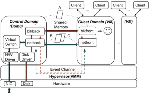
Xen provides a spectrum of virtualisation modes, where paravirtualisation (PV) and full vir-tualisation, or hardware-assisted virtualisation (HVM), are the poles. The main difference between PV and HVM mode is that, a paravirtualised guest “knows” it is being virtualised on Xen, contrary to a fully-virtualised guest. To boost performance, fully-virtualised guests can use special paravirtualised device drivers, and this is usually called PVHVM or PV-on-HVM drivers mode. Xen project 4.5 introduced PVH for Dom0 (PVH mode). This is essentially a PV guest using PV drivers for boot and I/O5.
The entire Xen kernel has been modified to replace privileged instructions with hypercalls, i.e. direct calls to the hypervisor. A domain is one of the VMs that run on the system. A hypercall is a software trap from a domain to the hypervisor, just as a system call is a software trap from an application to the kernel6. So, instead of issuing a system call to, for example, allocate a memory address space for a process, the PV guest will make a hypercall directly to Xen. This procedure is detailed in Figure 2.3. Domains will use hypercalls to request privileged operations. Like a system call, the hypervisor communicates with guest domains using an event channel. An event channel is a queue of synchronous hypervisor notifications for the events that need to notify the native hardware.
The reason for this mechanism is that, before hardware-assisted virtualisation was invented, the CPU would consider the guest kernel to be an application and silently fail privileged calls, crashing the guest. With hardware support and the drivers in Dom0, we can run the guest as a paravirtualised machine which allows the guest kernel to make the privileged call. The
5Xen Project Software Overview. http://wiki.xen.org/wiki/Xen_Project_Software_Overview 6Hypercall. http://wiki.xenproject.org/wiki/Hypercall
2.4. Characterising Performance Interference Caused by Virtualisation 17 Hypervisor(VMM) NIC Hardware Packets N/W Driver Virtual Switch Control Domain (Dom0) blkback Guest Domain (VM) Event Channel Disk ... (VM) Client ... netback Shared Memory A B C ... Client Client Client blkfront netfront Disk Driver
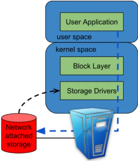
Figure 2.3: Xen hypervisor architecture with guest VMs
hardware will understand the call comes from a guest kernel (the guest domain or DomU) and trap it. It will then pass it to Xen, which in turn will invoke the same hypercall to, for example, update the page table or issue an I/O request [BDF+03] as shown in Figure 2.3. This avoids having to translate general system calls into specific calls to the hypervisor as in the HVM case. PV is very efficient and lightweight compared to HVM and hence it is more widely adopted as a virtualisation solution [XBNJ13, NKG10]. This is why we focus on modelling Xen’s PV mode.
We continue our discussion of the Xen internals with the credit-based CPU scheduler, followed by the grant table mechanism, and give more detail about the disk and network I/O data paths in Xen.
2.4.2
CPU Scheduler
When a VM is launched, the control domain will tell the hypervisor to allocate memory and copy the VM’s boot code and kernel to that memory. From this point, the VM can run on its own, scheduled directly by the hypervisor. The Xen hypervisor supports three different CPU schedulers which are (1) borrowed virtual time, (2) simple earliest deadline first, and (3)
credit scheduler. All of these allow users to specify CPU allocation via CPU shares (i.e. weights and caps). Credit scheduler is the most widely deployed Xen CPU scheduler after Xen 3.0 was released, because it provides better load balancing across multiple processors compared to other schedulers [CG05, CGV07, PLM+13].
The credit scheduler is a proportional fair-share CPU scheduler designed for SMP hosts7. The
‘credit’ is a combination effect of weight, cap and time slice. A relative weight and a cap are assigned to each VM. A domain with a weight of 512 will get twice as much CPU as a domain with a weight of 256 on the same host. The cap optionally fixes the maximum proportion of CPU a domain will be able to consume, even when the host is idle. Each VM is given 30 ms before being preempted to run another VM. After this 30 ms, the credits of all runnable VMs are recalculated. All VMs in the CPU queues are served as FIFO and the execution of these virtual CPUs (vCPUs) ends when the VM has consumed its time slice. The credit scheduler automatically load balances guest vCPUs across all available physical CPUs (pCPUs); however, when guest domains run many concurrent workloads, a large amount of time in the scheduler is spent switching back and forth between tasks instead of doing the actual work. This causes significant performance overhead.
A VM can enter a boost state which gives the VM a higher priority to be inserted into the head of the queue in case it receives frequent interrupts. These effects of the credit scheduler should be taken into consideration when analysing the performance of co-resident applications, as it is more likely to prioritise an I/O-intensive workload while unfairly penalising CPU-intensive workloads with higher processing latencies. For example, we also observe that executing a CPU-intensive workload within a VM alongside a network-intensive benchmark will result in better throughput for the network-intensive workload. However, to keep our model simple, this work does not consider this effect. We consider CPU-intensive and I/O-intensive (including disk and network) applications are allocated an equal share of CPU resources. We acknowledge this might account for part of the prediction errors observed in Section 5.5.
2.4. Characterising Performance Interference Caused by Virtualisation 19
2.4.3
Disk I/O
While CPU-intensive applications generally exhibit excellent performance (close to bare metal) on benchmarks, applications involving I/O (either storage or network) differ. When a user application inside the guest VM makes a request to a virtual disk, almost every process in the kernel behaves as in the case of a bare metal machine: the system call is processed; a corresponding request for a block device is created; the request is placed in the request queue and the device driver is notified to process the queue. From there, the driver passes the request to the storage media such as a locally attached disk (e.g. SCSI, SATA) or a network-based storage (e.g. NFS, iSCSI). Within a hypervisor, however, the device driver is handled by a module called blkfront(see Figure 2.3).
blkfront has a shared memory page with another component called blkback in the control
domain. This page is used to place the requests that come to the request queue of the virtual device. Once the virtual request is placed,blkfrontnotifiesblkbackthrough an interrupt sent via the event channel. blkback will process the request that comes from blkfront and make another call to Dom0’s kernel. This, in turn, creates another I/O request for the actual device on which the virtual disk allocates. As the virtual disk for a VM can be in various locations, Dom0’s kernel is responsible for directing requests coming from blkback to the correct place. All these processes add processing overhead and increase the latency for serving I/O requests.
So the actual speed of I/O requests is dependent on the speed and availability of the CPUs of Dom0. If there are too many VMs performing intensive CPU workloads, the storage I/O data path can be significantly affected [PLM+13, SWWL14].
2.4.4
Grant Table
After a virtual device has been constructed, the guest VM shares a memory area with the control domain which it uses for controlling the I/O requests, the grant table8. The paravirtualised
protocol has a limitation on the amount of requests that can be placed on this shared page
between blkfront and blkback (see Figure 2.3). Furthermore, these requests also have a limitation on the amount of data they can address (the number of segments per request). These two factors lead to higher latency and lower bandwidth, which limits I/O performance. The guest will also issue an interrupt to the control domain which goes via the hypervisor; this process has some latency associated with it.
2.4.5
Network I/O
Xen has a database on the control domain which is visible to all VMs through the hypervisor. This is called XenStore9. When the control domain initialises a VM, it writes certain entries
into this database exposing virtual devices (network/storage). The VM network driver will read those entries and learn about the devices it is supposed to emulate. This is the same process as when a physical network card driver loads and examines the available hardware (e.g. PCI bus) to detect which interfaces are available. The Xen VM network driver, called netfront, will then communicate directly with another piece of software on the control domain,netback, and handshake the network interface.
In contrast to storage, there aretwo memory pages shared betweennetfront andnetback, each of which contains a circular buffer. One of these is used for packets going out of the guest operating system (OS) and another is used for packets going in to the guest OS from the control domain. When one of the domains (either the guest or the control) has a network packet, it will place information about this request in the buffer and notify the other end via a hypervisor event channel. The receiving module, eithernetfrontornetbackis then capable of reading this buffer and notifying the originator of the message that it has been processed. This is different to storage virtualisation in that storage requests always start in the guest (the drive never sends data without first being asked to do so); therefore, only one buffer is necessary between the control domain and guest domains.
Having presented a brief overview of multicore and virtualisation technology, in the next part of this chapter, we will introduce the theoretical background of this dissertation.
2.5. Stochastic Modelling 21
2.5
Stochastic Modelling
To abstract a sequence of random events, one can model it as a stochastic process. Stochastic models play a major role in gaining insight into many areas of computer and natural sci-ences [PN16]. Stochastic modelling concerns the use of probability to model dynamic real-world situations. Since uncertainty is pervasive, this means that this modelling technique can potentially prove useful in almost all facets of real systems. However, the use of a stochastic model does not imply the assumption that the system under consideration actually behaves randomly. For example, the behaviour of an individual might appear random, but an interview may reveal a set of preferences under which that person’s behaviour is then shown to be en-tirely predictable. The use of a stochastic model reflects only a practical decision on the part of the modeller that such a model represents the best currently available understanding of the phenomenon under consideration, given the data that is available and the universe of models known to the modeller [TK14].
We can describe the basic steps of a stochastic modelling procedure as follows:
1. Identify the critical features that jointly characterise a state of the system under study. This set of features forms the state vector.
2. Given some initial states, understand the universe of transitions which occur between states, together with the corresponding probabilities and/or rates. The set of all states that can be reached from the initial state is known as the reachable state space.
3. Analyse the model to extract the performance measurements of interests, for example, the long run proportion of time spent in end state, or the passage time distribution from one set of state to another.
2.5.1
Discrete-time Markov Chains
Consider a discrete-time random process {Xm, m = 0,1,2, . . .}. In the very simple case where
there is no memory in the system so each Xm can be considered independently from previous ones. However, for many real-life applications, the independence assumption is not usually valid. Therefore, we need to develop models where the value of Xm depends on the previous
values. In a Markov process, Xm+1 depends on Xm, but not any the other previous values X0, X1, . . . , Xm−1. A Markov process can be defined as a stochastic process that has this
property which is known as Markov property [PN16].
Markov processes are usually used to model the evolution of “states” in probabilistic systems. More specifically, consider a system with a state spaceS ={s1, s2, . . .}. IfXn=i, we say that
the system is in state iat timen. For example, suppose that we model a queue in a bank. The state of the system can be defined as the non-negative integer by number of people in the queue. This is, ifXndenotes the number of people in the queue at timen, thenXn∈S ={0,1,2, . . .}. A discrete-time Markov chain is a Markov process whose state spaceS is a finite or countable set, and whose time index set isT ={0,1,2, . . .}[PN16, TK14]. In formal terms, Discrete-time Markov chains satisfy the Markov property:
P(Xm+1 =j | Xm =i, Xm−1 =im−1, . . . , X0 =i0) = P(Xm+1 =j | Xm =i),
for all t ∈ {0,1,2, . . .}, where P(Xm+1 = j | Xm = i) are the transition probabilities. This
notion emphasises that in general transition probabilities are functions not only of the initial and final sates, but also of the time of transition. When the one-step transition probabilities are independent of the time variable m, the Markov chain is said to be time-homogeneous [TK14] and P(Xm+1 = j | Xm = i) = pij. In this dissertation, we limit our discussion to this
case. As it is common in performance modelling Markov chains are frequently assumed to be time-homogeneous. When time-homogeneous, the Markov chain can be interpreted as a state machine assigning a probability of hopping from each state to an adjacent one, so that the process can be described by a single, time-independent matrix P = (pij), which will be
introduced in the next section. It greatly increases the trackability of the underlying system. Also, it is easy to parametrise the model given the read measurement data.
2.5. Stochastic Modelling 23
2.5.2
Transition Matrix and State Transition Diagram
The matrix of one-step transition probabilities is given by P= (pij). For r states, we have,
P= p11 p12 . . . p1r p21 p22 . . . p2r · · · · · · · · pr1 pr2 . . . prr
where pij ≥0, and, for all i,
r
X
k=1
pik = 1
Consider an example with four states and the following transition matrix:
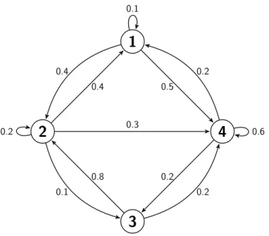
P= 1 10 2 5 0 1 2 2 5 1 5 1 10 3 10 0 45 0 15 1 5 0 1 5 3 5
Figure 2.4 shows the state transition diagram for the above Markov chain. The arrows from each state to other states show the transition probabilities pij. If there is no arrow from state i to statej, it means that pij = 0.
2.5.3
State Transition Probability Distribution
A Markov chain is completely defined once its transition probability matrix and initial state
X0 are specified (or, more generally, an initial distribution is given a row vector). Recall the
1
2
3
4
0.5 0.4 0.1 0.4 0.3 0.2 0.1 0.8 0.2 0.2 0.6 0.2Figure 2.4: A state transition diagram example
distribution of X0 is known. We can define the row vector π(0) as,
π(0) =P(X0 = 1), P(X0 = 2), . . . , P(X0 =r)
.
We can obtain the probability distribution ofX1,X2, . . . , at time step-n using the law of total
probability. More specifically, for any j ∈S, we have,
P(X1 =j) = r X k=1 P(X1 =j | X0 =k)P(X0 =k) = r X k=1 pkjP(X0 =k) If we define π(m) =P(Xm = 1), P(Xm = 2), . . . , P(Xm=r) ,
we can obtain the result,
π(1) =π(0)P,
Similarly,
2.5. Stochastic Modelling 25
The n-step transition probability of a Markov chain is,
p(ijn) =P(Xm+n=j | Xm =i) (2.1)
and the associated n-step transition matrix is
P(n) = (pij(n)) (P(1) =P).
The Markov property allows to express Equation 2.1 in the following theorem.
Theorem 2.1. The n-step transition probabilities of a Markov chain satisfy
p(ijn) = ∞ X k=0 pikp (n−1) kj (2.2) where we define p(0)ij = 1 if i = j, 0 otherwise.
From linear algebra we recognize the relation 2.2 as the formula for matrix multiplication, so that P(n) =P×P(n−1). By iterating this formula, we obtain
P(n)=P×P×. . .×P.
In other words, the n-step transition probabilities p(ijn) are the entries in the matrix Pn, the nth
power of P.
Proof. The proof proceeds via a first step analysis, a break down of the possible transitions, followed by an application of the Markov property. The event of going from state i to state j
afterntransitions can be realised in the mutually exclusive ways of going to some intermediate state k(k = 0,1, . . .) after the first transition, and then going from state k to state j in the remaining (n−1) transitions [HP92].
the first is pik. If we use the law of total probability, then Equation 2.2 follows [TK14]. The steps are, p(ijn) =P(Xn =j | X0 =i) = ∞ X k=0 P(Xn =j, X1 =k | X0 =i) = ∞ X k=0 P(X1 =k | X0 =i)P(Xn=j | X0 =i, X1 =k) = ∞ X k=0 pikp (n−1) kj
Letm and n be two positive integers and assume X0 =i. In order to get to statej in (m+n)
steps, the chain will be at some intermediate state k after m steps. To obtain p(ijm+n), we can obtain the Chapman-Kolmogorov equationover all possible intermediate states:
p(ijm+n) =P(Xm+n=j | X0 =i) =
X
k∈S
p(ikm)p(kjn)
2.5.4
Steady State and Stationary Distribution
Next we consider the long-term behaviour of Markov chains. In particular, we are interested in the proportion of time that the Markov chain spends in each state whennbecomes large [PN16]. A Markov chain’s equilibrium requires that: (i) the p(ijn) have settled to a limiting value; (ii) this value is independent of the initial state; and (iii) the π(jn) also approach a limiting value
πj [HP92].
Formally, the probability distribution π = [π0, π1, π2, . . .] is called the limiting distribution of
the Markov chain Xn. We have,
πj = lim
n→∞p
(n)
ij ,
for all i, j ∈S, with
X
j∈S
2.6. Queueing Theory 27 since, p(ijn+1) =X k p(ikn)pkj, as n→ ∞, πj = X k πkpkj, π = πP. (2.3)
As we can see theπ in Equation (2.3) is the left eigenvector of Pwith eigenvalue 1. Therefore, we can solve the limiting distribution by computing the eigenvector of the transition probability matrix P.
2.6
Queueing Theory
In many aspects of daily life, queueing phenomena may be observed when service facilities (counters, web services) cannot serve their users immediately. Queueing systems are mainly characterised by the nature of how customers arrive at the system and by the amount of work that the customers require to be served [Che07]. Another important characteristic is described as the service discipline, which refers to how the resources are allocated to serve the customers. The interaction between these features has a significant impact on the performance of the system and the individual customers.
The first queueing models were conceived in the early 20th century. Back in 1909, the Erlang loss model, one of the most traditional and basic types of queueing models, was originally developed for the performance analysis of circuit-switched telephony systems [Erl09]. Later, queueing theory was successfully applied to many areas, such as production and operations management. Nowadays, queueing theory also plays a prominent part in the design and performance analysis of a wide range of computer systems [Che07].
A queueing system consists of customers arriving at random times at some facility where they receive service of a specific type and then depart. Queueing models are specified as A/S/c,
according to a notation proposed by D. G. Kendall [Ken53]. The first symbol A reflects the arrival pattern of customers. The second symbol S represents the service time needed for a customer, and the ‘c’ refers to the number of servers. To fully describe a queueing system, we also need to define how the server capacity is assigned to the customers in the system. The most natural discipline is the first come first serve (FCFS), where the customers are served in order of arrivals. Another important type of queueing discipline arising in performance analysis of computer and telecommunication systems is so-called the processor-sharing (PS) discipline, whereby all customers are served in parallel [Che07, HP92]. In this dissertation, we use both disciplines to model systems of interest.
2.6.1
Important Performance Measures
Queueing models assist the design process by predicting and managing system performance. For example, a queueing model might be employed to evaluate the cost and benefit of adding an additional server to a system. The models facilitate us to calculate system performance measures both from the perspective of the system, e.g. overall resource utilisation, or from the perspective of individual customers, e.g. response time. Important operating characteristics of a queueing system include [HP92]:
• λ: the average arrival rate of customers (average number of customers arriving per unit of time)
• µ: the average service rate (average number of customers that can be served per unit of time)
• ρ: the utilisation of the system, indicating the load of a queue • L: the average number of customers in the system
• LQ: the average number of customers waiting in line
2.6. Queueing Theory 29
2.6.2
Processor-sharing Queueing Models
In the field of performance evaluation of computer and communication systems, the processor-sharing discipline has been extensively adopted as a convenient paradigm for modelling capac-ity sharing. PS models were initially developed for the analysis of time-sharing in computer communication system in the 1960s. Kleinrock [Kle64, Kle67] introduced the simplest and best-known egalitarian processor-sharing discipline, in which a single server assigns each customer a fraction 1/n of the server capacity whenn > 0 customers are in the system; the total service rate is then fairly shared among all customers present.
An M/M/1 queue is the simplest non-trivial queue where the requests arrive according to a Poisson process with rate λ, which is the inter-arrival times are independent, exponentially distributed random variables with parameter λ. The service time are also assumed to be independent and exponentially distributed with parameter µ. Similar to M/M/1-FIFO, the arrival process of an M/M/1-PS queue is a Poisson process with intensityλand the distribution of the service demand is also an exponential distributionExp(µ). Then the number of customers in the system obeys the same birth-death process as in the M/M/1-FIFO queue [Vir16]. With
n customers in the system, the queue length distribution of the PS queue is the same as for the ordinary M/M/1-FIFO queue,
πn = (1−ρ)ρn, ρ=λ/µ
Accordingly, the expected number of customers in the system,E[N], and by Little’s Law10, the expected delay in the system E[T] are,
E[N] = ρ
1−ρ, E[T] =
1/µ
1−ρ
10“Little’s law,” in Wikipedia: The Free Encyclopedia; available from https://en.wikipedia.org/wiki/
The average sojourn time of a customer with service demandx is:
T(x) = x
C(1−ρ)
where C is the capacity of the server. This means that jobs experience a service rate of
C(1−ρ) [HP92, Vir16].
2.6.3
BCMP Network
Queueing networks are the systems in which individual queues are connected by a routing network. In the study of queueing networks one typically tries to obtain the equilibrium dis-tribution of the network11. However, so as to enable computation of performance metrics such as throughput, utilisation and so on, attempting to solve for the steady state distribution of all queues joint often proves intractable on account of the state space explosion problem. For efficient solution, separable approaches that analyse queues in isolation and then combine the results to obtain a joint distribution are necessary. The leading example of this is the BCMP theorem which defines a class of queueing networks in which the steady state joint probability distributions have a product form solution. It is named after the authors of the paper where the network was first described [BCMP75]: Baskett, Chandy, Muntz and Palacios. The theorem was described in 1990 as “one of the seminal achievements of queueing theory in the last 20 years” by J.M. Harrison and R.J. Williams in [HW90].
Definition of a BCMP network. A network of m interconnected queues is generally iden-tified as a BCMP network if each of the queues is one of the following four types:
1. FCFS with class-independent exponentially distributed service time
2. PS queue
3. IS (Infinite Server) queue
11“Queueing theory,” in Wikipedia: The Free Encyclopedia; available from https://en.wikipedia.org/
2.6. Queueing Theory 31
4. LCFS (Last Come First Serve) with pre-emptive resume
In the final three cases, the service time distribution must have a rational Laplace trans-form [HP92]. That is,
L(s) = N(s)
D(s)
where N(s) and D(s) are polynomials in s. Also, it must meet the following conditions:
• External arrivals to node i (if any) follow a Poisson process.
• A customer completing service at queue i will either move to some new queue j with (fixed) probabilitypij or leave the system with probability 1−
PM
j=1pij, which is non-zero
for some subset of the queues12.
Also it is assumed that the routing of jobs among queues is state-independent. That is, jobs are routed among the queues according to fixed probabilities (which could be different for different classes of jobs) and not based on the number of jobs in the queues. Then the steady-state joint probability distributionπn1n2...nM is of the form,
πn1n2...nM = π1(n1)π2(n2). . . πM(nM)
K
where πm(nm) is the stationary probability of observing nm jobs in queuem if the queue were
in isolation with a Poisson input process having the same rate as the throughput for queue m, and K is a normalisation constant [HP92]. In the case of an open network,K is always 1. For a closed network, K is determined by the constraint that the state probabilities sum to 1,
K = X
all states
π1(n1)π2(n2). . . πM(nM)
12“BCMP network,” inWikipedia: The Free Encyclopedia; available fromhttps://en.wikipedia.org/wiki/
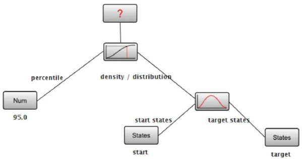
Figure 2.5: An example of Performance Tree query: “what is the 95th percentile of the passage time density of the passage defined by the set of start states identified by label ‘start’ and the set of target states identified by label ‘target’ ?
2.7
Performance Trees
Finding a way to represent complex performance queries on models of systems in a way that is both accessible and expressive is a major challenge in performance analysis [SBK06]. This section describes an intuitive way to address this challenge via the graphical Performance Trees (PTs) formalism. PTs are designed to be accessible by providing intuitive query specification, expressive by being able to reason about a broad range of concepts, extensible by supporting additional user-defined concepts, and versatile through their applicability to multiple modelling formalisms [KDS09]. Whereas PT queries can also be expressed in textual form [SBK06], the formalism was primarily designed as a graphical specification technique and we focus on this graphical interface to help performance management.
A PT query consists of a set of nodes that are connected via arcs to form a hierarchical tree structure, as shown in Figure 2.5. Nodes in a PT can be of two kinds: operation or value nodes. Operation nodes represent performance concepts and behave like a function, taking one or more child nodes as arguments and returning a result. Child nodes can return a value of an appropriate type or value nodes, which can represent other operations such as states, functions on states, actions, numerical values, numerical ranges or Boolean values. PT queries
2.7. Performance Trees 33
can be feasibly constructed from basic concepts by linking nodes together into query trees. Arcs connect nodes together and are annotated with labels, which represent roles that child nodes have for their parent nodes. The root node of a PT query represents the overall result of the query. The type of the result is determined by the output of the root’s child node while PTs are evaluated from the bottom-up [KDS09, SBK06]. For example, the bottom right of Figure 2.5 computes the probability density function (P