Leveraging over Prior Knowledge for Online Learning of Visual Categories across Robots MOHSEN KABOLI

(1)

Leveraging over Prior Knowledge

for Online Learning of Visual Categories

across Robots

(2)

Leveraging over Prior Knowledge

for Online Learning of Visual Categories

across Robots

M O H S E N K A B O L I

DD221X, Master’s Thesis in Computer Science (30 ECTS credits) Master Programme in Wireless Systems 120 cr

Royal Institute of Technology year 2012 Supervisor at CSC was Danica Kragic

Examiner was Danica Kragic TRITA-CSC-E 2012:053 ISRN-KTH/CSC/E--12/053--SE ISSN-1653-5715

Royal Institute of Technology

School of Computer Science and Communication KTH CSC SE-100 44 Stockholm, Sweden URL: www.kth.se/csc

(3)

Introduction

Abstract

Open ended learning is a dynamic process based on the continuous processing of new data, guided by past experience. On one side it is helpful to take advantage of prior knowledge when only few information on a new task is available (transfer learning). On the other, it is important to continuously update an existing model so to exploit the new incoming data, especially if their informative content is very different from what is already known (online learning). Until today these two aspects of the learning process have been tackled separately. In this thesis we propose an algorithm that takes the best of both worlds: we consider a sequential learning setting, and we exploit the potentiality of knowledge transfer with a computationally cheap solution. At the same time, by relying on past experience we boost online learning to predict reliably on future problems. A theoretical analysis, coupled with extensive experiments, show that our approach performs well in terms of the online number of training mistakes, as well as in terms of performance on separate test sets.

(6)

1.1 Introduction

Machine learning algorithms predict on the future data with the help of statistical models that are learned from collected labeled or unlabeled training sets [8],[19],[29]. In semi supervised classification [2],[16],[17], [32] labeled data are too few to build a good classification models, therefore using a large amount of unlabeled data together with a small amount of labeled data it is possible to find the good learning models for the classifiers. Many research in classification task have done by assuming that the distributions of the labeled and unlabeled data are the same. Knowledge transfer, in contrast, allows the domains, tasks, and distributions used in training and testing to be different. Knowledge transfer allows to exploit prior knowledge when learning a new class, which reduces the need for annotated training samples. Many works address the issue of what to transfer, for instance, samples of data [1], feature representation [4], model parameters [12], moreover, some focus on how to transfer [12], like, boosting [30], and SVM [7], while others concentrate on how to avoid negative transfer, evaluating when and how much to transfer or methods to measure the task relatedness [10]. In real world, we observe many examples of transfer learning for example, we may find that learning to recognize bicycle, might help to recognize motorbike or car rather than cat and dog. The fundamental motivation for knowledge transfer in the field of machine learning was discussed in a NIPS-95 workshop onLearning to Learn which focused on the need for lifelong machine learning methods that retain and reuse previously learned knowledge [22]. The main goal of all research in visual recognition is to enable vision-based artificial systems to operate autonomously in the real world. However, even the best system we can currently engineer is bound to fail whenever the setting is not heavily constrained. This is because the real world is generally too nuanced, too complicated and too unpredictable to be summarized within a limited set of specifications. There will be inevitably novel situations and the system will always have gaps, conflicts or ambiguities in its own knowledge and capabilities. This calls for algorithms able to support open ended learning of visual classes. The open ended learning issue, i.e. the ability to learn a new detected class continuously over time, has been typically addressed in a fragmented fashion in the literature. A first component is that of transfer learning, i.e. the ability to leverage over prior knowledge when learning a new class, especially in presence of few training data [22]. A second component is that of being able to update continuously the learned visual class, as new samples arrive sequentially. The dominant approach in the literature here is that of online learning: predictions are made on the fly and the model is progressively updated at each step, on the basis of the given true label. An attractive feature of this family of algorithms is that they aim at minimizing the number of total mistakes on the incoming samples (mistake-bound). In this thesis we propose to merge together these two components, using the prior knowledge sources for initializing the online learning process on a new target task through transfer learning. This has two main advantages: (1) by using a principled transfer learning process we can study the relation between the old sources and the new target. Within this

(7)

1.2. RELATED WORKS

framework, few samples might be sufficient to indicate in which part of the original space the correct solution (the best in term of generalization capacity) should be sought. (2) we show theoretically that a good initialization for the online learning process produces a tighter mistake bound compared to previous work [31], while empirically improving the recognition performance on an unseen test set. Globally an expensive transfer learning approach is used only at the beginning, therefore limiting the computational burden. Then, a fast and efficient online approach is applied. We choose the Passive Aggressive online learning algorithm [5], and we show how to initialize it in two different fashions with a state of the art transfer learning method [25]. For each of the two versions of the algorithm, we derive the relative mistake bound, which provide us with a deeper understanding of the methods. Experiments on the object categorization domain show the potential of our approach.

1.2 Related Works

To our best of knowledge, the most similar approach to our methods has introduced by Zhao and Hoi in OTL (A Framework of Online Transfer Learning) [31] which is based on ensemble learning, it makes a prediction of online learning function with the help of PA-algorithm [5] on the data of the target domain, and combine it with the old prediction function learned on the prior knowledge. The weights for the combination of prediction function are adjusted dynamically on the basis of a squared loss function which evaluates the difference among the current prediction and the correct label of any new incoming sample. OTL algorithm cannot exploit multi prior knowledge and authors just introduced a theoretical analysis for single prior knowledge model which demonstrates the existence of a mistake bound for their algorithm. In contrast, our proposed methods are able to transfer from multi-ple sources. Moreover we will show that the bound on mistakes in case of exploiting both single and multi prior knowledge do not behave worse than the OTL. In addi-tion, to be able to compare our results in case of multi source transfer learning we modified OTL algorithm to be able to transfer multi prior knowledge (4.1.4).

(8)

1.3 Contribution and Organization of this Thesis

In this thesis we proposed two novel online transfer learning methods that aim to transfer knowledge from some source domains to an online learning task with differ-ent classes in both target and source data. We call our suggested methods TROL and TROL+ . In TROL technique (4.1.1) we propose initializing of the online learning algorithm with the help of Multi-KT method [25] which provides a model for the new target problem on the basis of very few training samples exploiting a reliable combination of sources. In second method , TROL+ (4.1.3) we suggest re-weighting the old knowledge during online integrating prior and new knowledge together. We show that it is possible to employ a simple augmentation trick to have the same starting condition of TROL together with a progressive update of old and new knowledge weights in time. One important issue in our research which raises the challenge of knowledge transfer is to address concept drifting problem. It means that the new samples to be predicted changes over time in learning process. Moreover, to compare our techniques with OTL method as the only close work to ours, in case of employing multi class prior knowledge, we needed to modify the OTL to be able to use multiple sources as the original algorithm cannot. We called the modified version of OTL algorithm M-OTL (4.1.4). We show also the mistakes bounds of the proposed algorithm, and empirically examine our methods with some available baselines.

This thesis is organized as follows : Chapter 1 includes an introduction to our research followed by description of some related works, chapter 2 explains some definition of transfer learning and reviews online learning methods , in chapter 3 we discuss batch transfer learning together with online transfer learning algorithms, chapter 4 presents our proposed methods, chapter 5 gives experimental results , and chapter 6 concludes this thesis and our research.

(9)

Chapter 2

(10)

2.1 Knowledge Transfer

2.1.1 Motivation

Most traditional machine learning algorithms are invented based on training and testing data sample with same feature space and distribution domain. On the contrary, knowledge transfer makes new target learning algorithms able to exploit the pre-trained knowledge from the previous tasks with different distribution and feature space. In other words, knowledge transfer method allows to employ prior knowledge when learning a new class, which in both supervise and semi supervise learning approach reduces the need for labeled training data. Figure (2.1) shows different learning process between traditional learning and knowledge transfer.

Figure 2.1. Different learning process between traditional learning and transfer learning [22]

2.1.2 Definition of Knowledge Transfer and Some Notation

Domain D has two elements one is feature space, x = {x1, ....,xn} ∈ X, and the

other is marginal probability distribution,P(x). Different domainD_s means differ-ent either in the feature space for instance, differdiffer-ent feature descriptors in object recognition issue or different in the marginal probability distribution for example, different class of objects in object categorization task. A Task T, in knowledge transfer consists of a label space, and objective predictive function f(.). Different task, means either different in objective predictive function f(.) (different condi-tional probability distribution ) for instance, the situation in which the source and target objects in object recognition issue are very unbalanced in term of the user defined classes, or different in label space Y for instance in situation where source domains has binary classes whereas the target domain is multi-class [22].

(11)

2.1. KNOWLEDGE TRANSFER

2.1.3 Related and Unrelated Domain

The source domains and target domains are related when implicitly or explicitly,

there exists some relationship between feature spaces otherwise areunrelated [22].

2.1.4 Important Issues in Knowledge Transfer Techniques

In the field of knowledge transfer, researchers are concern about finding the proper and clear answer for the following issues : what to transfer,how to transfer, andwhen

to transfer [26]. What to transfer means to discover which part of knowledge makes

an improvement of performance in domains and targets and is worth to transfer. To develop the learning algorithm to transfer the knowledge corresponds to thehow

to transfer. When to transfer means in which situation transferring the knowledge

helps to improve the performance of learning in target and when transferring the knowledge by negative transferring hurts the performance of learning due to the unrelated domain and target source [22].

2.1.5 Categorization of Knowledge Transfer

Transfer learning is classified into three different settings: (1)Inductive Transfer

Learning,(2)Transductive Transfer Learning, and (3)unsupervised transfer learning.

Moreover, based onwhat to transfer in learning, each approaches is categorized into four contexts. (1)Instance Transfer approach, (2)Feature Representation Transfer

approach, (3)Parameter Transfer approach, (4)Relational Knowledge Transfer ap-proach. In following we explain the different approaches of the transfer learning [22].

2.1.6 Inductive Knowledge Transfer

Inductive transfer learning tries to ameliorate the learning of the target learning functionf(.) in D_T exploiting the knowledge inD_s and T_s, in which T_s6=T_T [22].

Instance Transfer Approach

In this approach, it is not possible to utilize source domain directly in the target domain, but there are some particular parts of the data that can be exploited with

(12)

Feature Representation Transfer Approach

The goal of feature representation transfer approach is to find the suitable feature representations to reduce domain divergence and classification model error. The procedure of discovering the appropriate feature representations are different for various types of the source domain data [22].

Parameter Transfer Approach

In this approach the individual models for related tasks share some parameters or prior distributions of hyper parameters. The majority of the approaches are designed to work under multitask learning by easily changing the regularization structure [22].

Relational Knowledge Transfer Approach

This technique of knowledge transfer is alien to previous approaches and data are not independent and identically distributed (i.i.d) so it can be delineated by multiple relations, which means that is not essential data in each domain to be (i.i.d ) [22].

2.1.7 Trnsductive Knowledge Transfer

Transductive transfer learning attempts to ameliorate the learning of the target leaning function f(.) in DT employing the knowledge in Ds and Ts, where Ts =TT and Ds 6= DT. Moreover, there must be some unrelated target domain data at training time [22].

Instance Transfer Approach

The purpose of this idea is to learn an optimal model for the target domain by reducing the expected risk, in addition there is not any annotated training samples in the target domain, therefore, the models should be learned just by the source domain data [22].

Many researches in this approach have done under unsupervised learning frame-works [22].

(13)

2.1. KNOWLEDGE TRANSFER

2.1.8 Unsupervised Knowledge Transfer

Unsupervised transfer learning tries to gain the learning of the target functionf(.) inD_T employing the knowledge in D_s and T_s, whereT_s6=T_T and labels of training samples in both source and target domains are not accessible. In unsupervised transfer learning, the predicted labels are possible variables [22].

This perspective of knowledge transfer attempts to clustering a small group of un-labeled data in the target domain by employing a large amount of unun-labeled data in the source domain. Theses techniques are studied by [28].

In figure (2.2) we summarize all different setting of Transfer Learning.

Transfer Learning Transfer Learning Unsupervised Transfer Learning Unsupervised Transfer Learning Inductive Transfer Learning Inductive Transfer Learning Transductive Transfer Learning Transductive Transfer Learning Case1 Case1 Case2 Case2 No labeled data in a source domain

No labeled data in a source domain

Labeled data are available in a source domain

Selftaught Learning Selftaught Learning No labeled data in both source and target domain No labeled data in both source and target domain Labeled data are available Labeled data are available only in a source domain only in a source domain Labeled data are available Labeled data are available only in a source domain only in a source domain Labeled data are available in a target domain Labeled data are available in a target domain Multitask Learning Multitask Learning Domain Adaptation Domain Adaptation Sample Selection Bias Covariance Shift Sample Selection Bias Covariance Shift Source and targets are learnt simultaneously Source and targets are learnt simultaneously Assumption: single domains and single task Assumption: single domains and single task Assumption: different domains but single task Assumption: different domains but single task

(14)

2.1.9 Negative Transfer

Most approaches to transfer learning assume transferring knowledge across domains be always positive. However, in some cases, when two tasks are too dissimilar, brute-force transfer may even hurt the performance of the target task, which is called negative transfer [21].

(15)

2.2. OVERVIEW ON ONLINE LEARNING

2.2 Overview on Online Learning

A common trend in machine learning is the employment of huge amounts of data to achieve an increase in classification performance. Cognitive systems learn con-tinuously from experience, updating their models of the environment. This learning strategy is the main purpose why cognitive systems are capable of achieving a ro-bust, still adaptable ability to respond to new stimuli. Moreover, in real world many problems are fundamentally sequential and information will not be accessible at the same time. Sometimes the learned implication will revolve over time. For instance an autonomous robots need to learn continuously from their adjacency, to adapt to the ever changing surroundings. This interesting example needs learning algorithms capable to update their internal delegation which is antagonized to the traditional batch learning algorithms. Many times updating the solution is con-ceivable only via a thorough re-training, employing the training set including with the existing samples and the new training samples. The algorithms expanded in the online learning structure are fundamentally brought forth to be updated after each sample is received. Therefore, we conclude that online updating is a vital component for learning algorithms using in artificial intelligent systems. From com-putational complexity perspective, online learning algorithm has extremely lower mathematical complexity than batch learning methods. In machine learning field, recently many strong online learning algorithm have been proposed [23] with the ability of employing different regularizers to minimize the objective loss function effectively. With the aid of the offered methods, we can draw expedient online learning methods to find the solution for complex batch learning issues. In the following, concurrently we look at the issue from passive-aggressive online learning algorithm and optimization perspective (2.2.2).

2.2.2 Passive Agressive Algorithm

The passive-aggressive (PA) algorithm was proposed by Crammer and his colleagues in 2006 [5]. PA-algorithm is a margin based online learning algorithm to estimate different classification tasks which observes instances in a sequential manner. Online algorithm is usually simple to implement and their analysis often provides tight bound on their proficiency. Although PA-algorithm utilizes hypothesis from the set of linear prediction by using Mercer kernels one can employ highly non-linear prediction with still keeping the formal attributes and simplicity of linear predictor.

(16)

update of the algorithm is carried out by solving a confined optimization function by keeping the new classifier as close as possible to the current models of classifier while getting at least a unit margin on the most recent instances. The general structure of PA-algorithm can be viewed as discovering a Support Vector based on the single training sample while changing the norm of SVM with almost constraint to the current classifier. This method has two advantages. (1) To have close form solution for the next classifier and (2) to provide a unified analysis of the cumulative loss for different online classification.

Problem Setting

Online binary classification participates in a sequence of rounds. On each round the algorithm perceives one sample and estimates its related label with the aid of pre-learned hyper models from previous observed examples. PA- algorithm makes correct prediction if the corresponding margin in each round is grater than one oth-erwise, it suffers an instantaneous loss which is defined by hinge-loss function. In addition, classifier uses the newly obtained instance-label pair to improve its pre-diction for the next rounds. The confidence of the prepre-diction in each round, can be shown by |w.x|. PA-algorithm learns weight vectorwincrementally and observes a new training sample and weight vector time to timet. In PA-algorithm hinge loss function is used to calculate the missclassification as [5] :

`(w; (x,y)) = max(0,1−y(w.x)) (2.1)

Binary Classification Algorithms

How to initialize the weight vector is very important in both obtaining a concrete algorithm and defining the update rule to modify the weight vectorw_tat the end of each roundt. In this section we present three different update rules in case of binary classification. We name them as PA , PAI , and PAII . In all different update rules the weight vector w₁ is initialize with (0,...,0), on round t the new wight vector

w_t₊₁ is the solution of the following constrained optimization function [5] :

w_t+1 = min w∈Rd 1 2kw−wtk 2 _s.t _`₍_w_{; (}_x t,yt)) (2.2)

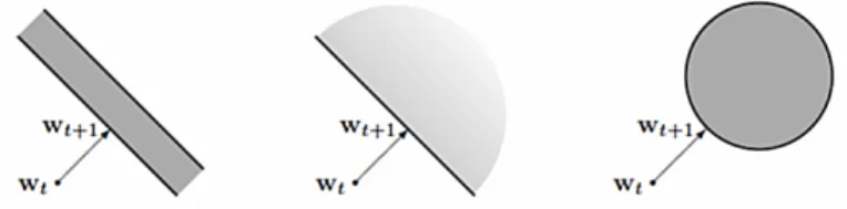
Geomatrically,wt+1 is set to be the projection ofwton to the half-space of vectors which attains hinge-loss of zero on the current instance. If the hinge-loss is zero then

(17)

w_t₊₁ = w_t, therefore the loss function is also zero `t = 0. Fig.(2.3). The solution to the optimization problem in Eq.(2.2) has a simple close form as in following :

w_t₊₁=w_t+τtytxt where τt=

`t

kx_tk2 (PA) (2.3)

If`t= 0 thenwt, itself satisfies the constraining Eq.(2.2) and it is optimal solution of optimization problem. If`t> 0 , then the Lagrangian cost function of Eq.(2.2) is:

L(x, τ) = 1

2kw−wtk

2₋_τ₍₁₋_y

t.xt). (2.4)

whereτ ≥0 is a Lagrangian multiplier.

The optimization problem Eq.(2.2) has a convex objective function and a single affine constrain which are enough to hold the Slater’s condition to find the optimum solution which is equivalent to satisfying the Karush-Khun-Tucker’s condition(Boyd and Vanderberghe,2004). By setting the partial derivatives of Lequal to zero with respect to the elements of w, we get [5] :

0 = ∇_wL(w, τ) = w−w_t−τ ytxt =⇒ w = wt + τtyt.xt (2.5)

By substituting the above result into Eq.(2.4) we get :

L(τ) = −1

2τ

2_k_x

tk2 + τ(1−yt(wtxt)) (2.6)

By taking the derivative of L(τ) with respect toτ and setting to zero, we get:

0 : = ∂L(τ) ∂τ = −τkxtk 2 _{+ (1}₋₍_y twtxt)) =⇒ τ = 1−yt(wtxt) kxtk2 (2.7)

Since `t > 0, we have `t = 1−yt(wt.xt) , therefore, we can write a uniform

up-date for the case where `t= 0 , and also the case where`t >0 , just by setting

(18)

In PA-algorithm, updating the weight vector satisfies the constrain aggressively by imposing the current sample which may result undesirable consequences. In other word, PA-algorithm updates weight vector in time of observing a new sam-ple, therefore, any miss classification due to label noise in data set may cause sever change in weight vector with the result of the wrong direction of hyperplane and it means that having several prediction mistakes on subsequent rounds. PA-algorithm introduces two techniques to solve this problem. The original idea of these tech-nique comes from soft margin classifier in support vector machine (Vapnik 1998) by introducing a non-negative slack variable ξ in optimization objective function Eq.(2.2). In first method the optimization objective function is scaled withξ.

wt+1= min w∈Rd 1 2kw−wtk 2 +Cξ s.t. `(w; (xt,yt))6ξ and ξ ≥0 . (2.8)

Parameter C in (2.8) is positive value which governs the influence of the slack terms. Large value of C implies more aggressive update in algorithm. This technique is known as a PAI [5].

In second technique, objective cost function is scaled quadratically withξ. since ξ2

is always non-negative there is no need for constraint ξ ≥ 0. This update method is known as PAII [5]. wt-1= min w∈Red 1 2kw−wtk 2₊_Cξ2 _s.t. _`₍_w_{; (}_x t,yt))6ξ . (2.9)

The solution to optimization problem in Eq.(2.8) and Eq.(2.9) has a simple unified close form for all update techniques.

wt+1 =wt+τtytxt (2.10) Where : τt= `t kxtk2 in (PA), τt= min{C, `t kxtk2 } in (PAI), τt= `t kxtk2+₂1_C in (PAII) (2.11)

All discussion till now was limited to linear prediction of the form sign(w.x). By using Mercer kernel we can generalize PA-algorithm as non-linear classifier. For all three different PA update we can write [5] :

(19)

Figure 2.3. An illustration of the update: wt+1is found by projecting the current

vectorwt onto the set of vectors attaining a zero loss. This set is a stripe in the case

of regression, a half-space for classification, and a ball for uni class [18].

wt= t−1 X i=1 τiyixi (2.12) and therefore: wtxt = t-1 X i=1 τiyi(xi.xt) (2.13)

The inner product of Eq.(2.13) can be replaced with a general Mercer Kernel

K(x_i.x_t). wtxt= t−1 X i=1 τiyiK(xi,xt) (2.14) Analysis of PA-Algorithm

In PA-algorithm the cumulative squared hinge loss upper bounds the number of prediction mistakes. The bounds in PA-algorithm prove that for any sequence of training samples this algorithm cannot work worse than the best fixed predictor. Since we are using PAI update in our project we will show just mistake bound for PA-algorithm in following [5].

(20)

Theorem :

Let (x1, y1), ...,(xT, yT) be a sequence of samples where xt ∈ Rn , yt ∈ {+1,−1} and kx_tk ≤ R for all t. Then, for any vector u ∈ Rn, the number of prediction mistakes made by PAI on this sequence of example is bounded from [5]:

max{R2, 1 C}(kuk 2_{+ 2}_C T X t=1 `(u; (x_t, yt))) (2.15)

(21)

Chapter 3

Batch Transfer Learning and Online

Transfer Learning

(22)

3.1 Batch Transfer Learning

Suppose we are given n different visual categories, the task is to distinguish each classes from background. Therefore, we should determinendifferent learning func-tions ni(x) → {1,−1} , with i = 1, ..., N such that the object x is set to be in the ith class if and only if ni(x) = 1. Now we would like to learn a new learning function fn+1 to classify a new n+ 1 class in the situation that only one or few

instances together with some background samples are accessible. To obtain fn+1

we need to train our classifier just with the available training data, or taking the advantage of pre-trained learning function or model parameters. In other words, suppose the task is to learn from few examples, for instance the class car, having already learned the categories motorbike, trunk, horse, and dog with the aim to improve the results by transferring from car and motorbike, rather than transfer-ring from car or motorbike. The expectation is to get better results compared to transferring equally fromall known categories, might generate negative transfer. In general speaking, knowledge transfer can give three advantages [9] in comparison with traditional machine learning, see Figure (3.1). First advantage is to get the higher start means the initial performance is higher (one-shot learning) and the second one is to have higher slope it means that the performance grows faster, the last benefit is to achieve the higher asymptote which means the final performance is better. This kind of scenario motivates us to design a knowledge transfer algorithm able to find autonomously the best subset of known models from where to transfer. In the following we briefly review the LS-SVM (3.1.2) theory and how it can be used in a model adaptation framework [11] then we review how this approach can be formulated to derive a knowledge transfer algorithm that exploits source knowl-edge from only one of the n classes [24] and at the end we extend this method to employ all the appropriate old knowledge [25]. Since we are utilizing a batch of data sample to find the bet learning models, we call our developed techniques as

Batch TRansfer Learning.

3.1.2 Least Square Support Vector Machine (LS-SVM) Definition

Least Square Support Vector machine (LS-SVM) is a Kernel based learning meth-ods. This algorithm is interesting because it can be employed as a strong non linear classifier just by utilizing simple mathematical methods. Suppose we have a binary problem with a set of l number of training samples {xi, yi}li=1 in which

xi ∈ X ⊂Rd is an input vector expressing the ith sample and yi ∈ Y ={−1,1} is the related label. The goal is to design a linear model function in a fixed feature

(23)

3.1. BATCH TRANSFER LEARNING

Figure 3.1. Three ways in which transfer might improve learning [26].

space which can distinguish correctly the unseen test sample x[6] :

f(x) =w·φ(x) +b (3.1)

where φ(x) is used to map the input samples to a high dimensional feature space Φ :X → F, induced by a kernel function :

K(x,x0) =φ(x)·φ(x0) (3.2)

In LS-SVM the model parameters (w, b) are found by solving the following op-timization problem [11]: min w,b 1 2kwk 2₊ C 2 l X i=1 [yi−w·φ(xi)−b]2 (3.3)

where C is a regularization parameter governing the bias-variance trade-off [6]. The precision of LS-SVM on unseen test data depends on discovering optimum values for the hyper-parameters which in our case are regularization parameter C

and kernel parameters. Looking for the optimum values of hyper-parameters are named as model selection. It can be shown that the optimal w is expressed by

w = Pl

i=1αiφ(xi). The corresponding primal Lagrangian for this optimization problem gives the following unconstrained minimization problem [6]:

(24)

where :

α= (α1, α2, . . . , αl)∈Rl (3.5)

is a vector of Lagrange multipliers and can be found by the solving the regularized least-squares problem (3.3) with a computational complexity of O(3) operations. The optimality conditions for the problem (3.4) is expressed by a linear equations that can be written concisely in matrix form as follows [3]:

" K+_C1I 1 1T 0 # " α b # = " y 0 # (3.6)

In Eq.(3.6), K depicts a kernel matrix. Suppose G delineates the first term in left-hand side of (3.6). Therefore the least-square optimization problem [3] can be solved just by simply inverting G. As previously mentioned the accuracy of the models on unseen test data is substantially depends on selecting the good learning parameters (e.g. the kernel parameters and the regularization parameter C can be found by a preceding cross validation considering the leave-one-out error. The LOO error is an unbiased estimator of the classifier generalization error and can be evaluated employing knowledge already accessible as a by-product of training the least-squares support vector machine on whole data set, with only a insignificant extra computational costs [3] [20]. Regarding to the equation (3.6) it is possible to show :

[α(−i), b(−i)]T =G(−i)−1[y1, ..., yi−1, yi−2, .., yl,0]T (3.7)

which shows the dual parameters of the LS-SVM when the ith sample is excluded during the leave-one-out cross validation procedure. With the aid of block matrix inversion lemma we can write the leave-one-out errorr_i(−i)for theithsample in close form.[3] [6]:

r(−_i i)=yi−ybi =

αi

G−1_ii . (3.8)

(25)

explicitly running cross validation experiment it is possible to express a criterion er-ror to maximize the LS-SVM model generalization performance, therefore the best learning parameters are those reducing the following error:

ERR= l X i=1 Ψ{yir (−i) i −1} with Ψ = 1 1 + exp(γ∗z) (3.9)

3.1.3 Learning a new object category from many samples

We would like to learn a new category from a pre-trained learning models or in other words from a set of annotated training data {x_i}_i₌₁_,m with the reward of exploiting what has been learned till now. To constrain a new model close to one of a set of pre-trained models [11] offered the technique which is mathematically formulated in the LS-SVM classification domain just by moderately changing the classical regularization part and expressing the following optimization problem :

min w,b 1 2kw−βw 0_k2₊C 2 l X i=1 ξ2 (3.10) subject to yi =w·φ(xi) +b+ξi ∀i ∈ {1,· · · , l}

Wherew0 is the parameter explaining the pre-traind model andβ is a scaling factor for governing the degree to which the new model is close to the old models or pre-trained models. w=βw0+ l X i=1 αiφ(xi) (3.11)

The optimum solution of modified objective cost function is given by the sum of the pre-trained model scaled by the parameterband a new model built on the new data points. If bequals to 0 in (3.10) we will get the original LSSVM formulation, which is without any adaptation to the previous data. To find the optimal β, [24] proposed to take benefit from the possibility of LS-SVM to write the leave-one-out

(26)

r_i(−i)= αi G−1_ii −β α0_i G−1_ii , (3.12) where α0_i =G−1₍₋_i₎[ˆy1, . . . ,yˆi−1,yˆi+1, . . . ,yˆl]T (3.13)

The G(−i) is the matrix attained when the ith sample is excluded in G and ˆyi = (w0·φ(xi)), it means ˆyi is the prediction of the old model on theith sample. With the aid of the new closed form of LOO for the modified cost function it is possible to discover best β for each known model, therefore by comparing all the criterion errors, the lowest one recognizes the best prior knowledge model to employ for adaptation.

3.1.4 Learning a new object category from few samples

We are given training samples with 1 positive and 10 negative instances and asked to assess from where to transfer with the aid of the leave one-out error. In such a situation just making one wrong prediction on one sample contributes for 1/10 of the total errors independently respect to the sign of its label. To utilize efficiently the criterion error is substantial to be more tolerant on negative sample due to their higher number, and strict on the positive sample which is alone. To cope with the effect of the unbalance contribution of training samples, re-weighting the leave-one-out recognition based on the number of the positive and negative samples is very promising. In the following we show the leave-one-out cross validation estimate of the Weighted Error Rate (WERR) by editing the criterion error [6] [3]:

W ERR= l X i=1 ζiΨ{yir(−_i i)−1} (3.14) Where : ζi= ( _l 2`+ if yi= +1 l 2`− if yi=−1 (3.15)

In equation (3.15), `+ and `− are the number of positive and negative instances respectively. ζ represents a weighting factor which is asymptotically equal to re-sampling the data, also the function Ψ is the same as (3.9). We suppose again our training set with 1 positive and 10 negative examples, and by employing the

(27)

Weighted Error Rate, the error on a negative example cooperates for 1/20 of the total while the error on the positive example contribute for 1/2. Without explicitly running cross validation experiments, the best learning parameters which maximize the LS-SVM model generalization performance can be found by minimizing WER and the lowest WER. The modified leave-one-out cross validation estimate of the Weighted Error Rate is named asAdapt-W. WERR gives concurring only in the last part of the transfer learning and it does not help to build the new adapted model which means that it is beneficial to choose the best prior knowledge to transfer and helps to define the relevance of the new task.To increase the robustness to unbal-anced distributions of the data, the model parameters (w, b) can be found through the minimization of a regularized weighted least-square loss function [6]:

min w,b 1 2kwk 2₊C 2 l X i=1 ζi[yi−w·φ(xi)−b]2 . (3.16)

The optimality condition for obtained problem (3.16) express a linear equation. The solution of this linear function results to discover the model parameter (α, b):

" K+_C1W 1 1T 0 # " α b # = " y 0 # , (3.17)

Where W = diag{ζ₁−1, ζ₂−1, . . . , ζ_l−1} and ζi are defined as in (3.15). Hence the model adaptation technique changes to its weighted formulation [24] :

min w,b 1 2kw−βw 0_k2₊C 2 n X i=1 ζi[yi−w·φ(xi)−b]2 subject to 0≤β ≤1 .

The weighting factors ζi take into account that the part of positive and negative examples in the training data are known not to be nominee of the operational class frequencies. Particularly, they help to balance the collaborating with the sets of pos-itive and negative examples to the data misfit term [24]. The proposed algorithm selects only one prior known model in time and is not always the best solution in a situation of exploiting multi prior models moreover, when the number of training samples increase, this method suffers from instability in time. Therefore we should find the new solution to cope with mentioned weakness points of [24]. The [25] solved the problems of [24] and proposed new method based on LS-SVM which is almost the modification of [24], in following we briefly explain this approach.

(28)

3.1.5 Multi Prior Transfer Learning

The [25] offered to replace the single coefficientβ with a vectorβ into the objective cost function (3.18) which contains as many components as the number of prior models,k : min w,b 1 2 w− k X j=1 βjw0j 2 +C 2 l X i=1 ζi(yi−w·φ(xi)−b)2 . (3.18)

Whereβ has to be selected in the unitary ball, it means kβk₂ ≤1. It is equated to the regularization term employed in LS-SVM in Equation (3.3), and it is a natural generalization of the original confine 0≤β ≤1 which is substantial to prevent high variance problems and happen when the number of known models are sufficient enough compared to the number of training samples. The new formulation of the optimal solution can be shown as :

w= k X j=1 βjw0j+ l X i=1 αiφ(xi) . (3.19)

where w is defined as a weighted sum of the pre-trained models scaled by the parametersβj, plus the new model built on the incoming training data. To discover the optimal β we utilize again the benefit of LS-SVM to write the LOO error in closed form: r(−_i i)=yi−y˜i = αi G−1_ii − k X j=1 βj α0_i₍_j₎ G−1_ii , (3.20) where α0_i₍_j₎=G−1₍₋_i₎[ˆy₁j, . . . ,yˆ_ij₋₁,yˆ_ij₊₁, . . . ,yˆj_l,0]T (3.21) and ˆ yj_i = (w0_j·φ(xi)) (3.22)

(29)

3.1. BATCH TRANSFER LEARNING yiy˜i= 1−yi   αi G−1_ii − k X j=1 βj α0_i₍_j₎ G−1_ii   . (3.23)

The best amount of βj are those reducing the LOO error, it means the values resulting positive amount foryiy˜i, for eachi. However minimizing directly the sign of those quantities would conclude in a non-convex formulation with lots of local minima. Therefore, we offer the following loss function :

loss(yi,y˜i) =ζimax [1−yiy˜i,0] = max

 y_iζ_i   αi G−1_ii − k X j=1 βj α0_i₍_j₎ G−1_ii  ,0   . (3.24)

This loss function is alike to the hinge loss exploited in Support Vector Machines. It is a convex upper bound to the LOO missclassification loss and favors solution in which ˜yi has a amount of 1, beside having the same sign of yi. Moreover it has a smoothing effect, similar to the function in (3.9). Finally, the objective function is: J = l X i=1 loss(yi,y˜i) s.t. kβk2 ≤1 . (3.25)

The above formulation is equivalent to the optimization problem of :

kβk2 2

2 + CJ (3.26)

for a proper choice of C [6]. The best values of βj to weight the known prior models can be find by minimizing J in the transfer learning process and scaling factorsζi are introduced in the loss function to take care of the data unbalance be-tween positive and negative samples in the training set, as in [24]. The optimization process the [25] utilizes a simple projected sub-gradient descent algorithm, in which at each iterationβ is projected onto thel2-sphere,kβk2 ≤1.

(30)

Properties

The main goal of the offered method is to transfer multiple models rather than only one, moreover in [25] the significance of the model and its interaction to prevent negative transfer knowledge are assessed at the same time, also the optimization of the loss function and objective function(3.25) has the unique solution as they are both convex function. In addition, the new formulation is firm enough which means that the behavior of the algorithm does not interchange much if one instance is excluded or included. We employ this algorithm as batch transfer learning in our proposed method (4.1.1), 4.1.3.

(31)

3.2. OTL: A FRAMEWORK OF ONLINE TRANSFER LEARNING

3.2 OTL: A Framework of Online Transfer Learning

3.2.1 Introduction

Zaho and Hoi proposed a new framework of online transfer learning (OTL) algo-rithm with the goal of improving supervised online learning algoalgo-rithm in a new target domain by employing the knowledge learned previously from some source domains. In this method, target variable to be predicted changes in learning pro-cedure over time and also both target and source domains can be variant in their feature representations and class distributions. In the following we explain briefly the OTL technique and its corresponding obtained mistake bound in situation that the source and target domains have the same feature space (homogeneous data).

3.2.2 OTL Algorithm

The OTL algorithm proposed in [31] is a two stages online learning approach which combines a source classifierh(x) with a prediction function f(x) learned online on the target domain. Specificallyf is learned from a sequence of samples (xt, yt) where

t∈ {1, . . . , T}. At the t−trial the learner receives an instancextand the prediction functionft is updated to ft+1 according to the PA-algorithm’s rule Eq.(2.10) with

ft(xt) = wt·xt. In addition, the corresponding class label is predicted by the following ensemble function [31] :

b

yt=sign(αtΠ(h(xt)) +γtΠ(ft(xt))− 1

2) (3.27) Where Π(x) = max{0,min{1,x+1₂ }} is a normalization function. The weights are initialized asα1 =γ1= 1₂ and at each step they are adjusted dynamically according

to [31] : αt+1 = αtst(h) αtst(h) +γtst(ft) γt+1 = γtst(ft) αtst(h) +γtst(ft) (3.28) where : st(g)= exp{−η`s(Π(g(xt)),Π(yt))} (3.29)

(32)

and `s(z, y) = (z−y)2 is the loss function. Here we would like to analyze the mistake bound in OTL method but we nee to introduce a preposition which will be employed in deriving the mistake bound later.

3.2.3 Preposition

When using the square loss function as `s(z, y) = (z−y)2 in which z ∈[0,1] and

y∈ {0,1}and the above weighting update technique and settingη= 1/2, the bound of the ensemble algorithm can be written as :

T X t=1 `s(αtΠ(h(xt)) + γtΠ(ft(xt)) , Π(yt)) ≤ 2 ln 2 + min n PT t=1 `s(Π(h(xt)) , Π(yt)) , PTt=1 `s(Π(ft(xt)) , Π(yt)) o

With the help of above proposition now we can derive the mistake bound of the OTL method in case of homogeneous target and source domains.

3.2.4 Theoretical Analysis

In the particular case of one single source task the OTL algorithm has a theoretical support given by the possibility to prove an upper bound on the number of mistakes made during the online learning process.

Theorem : Let us denote by M the number of mistakes made by the OTL algorithm, we have then M bounded from above by[31] :

M ≤4 min{Σ_h,Σ_f}+ 8 ln 2, (3.30) where: Σ_h = T X t=1 `s(Π(h(xt)),Π(yt)) (3.31) Σf = T X t=1 `s(Π(ft(xt)),Π(yt)) (3.32)

(33)

3.2. OTL: A FRAMEWORK OF ONLINE TRANSFER LEARNING

Note that the first stage in OTL is based on the PA-algorithm, that uses the hinge loss, while the second stage uses the square loss. Hence in [31] the Authors observe that, if we denote byMh andMf the mistake bound of the modelh andft respectively, and we assume that:

`s(Π(h(xt)),Π(yt))≈ 1 4Mh (3.33) and `s(Π(ft(xt)),Π(yt))≈ 1 4Mf (3.34) then M ≤min{Mh, Mf}+ 8 ln 2 (3.35)

The obtained mistake bound gives a powerful theoretical support to the OTL method. This algorithm can only employ single source knowledge to transfer. Hence, in case of multiple sources, it should be modified to be able to exploit multi prior knowledge. In this thesis we modify the OTL algorithm to exploit multi prior knowledge (4.1.4), then we compare performance of the modified OTL with our proposed methods. We will see that the performance of our methods and their corresponding mistake bound outperform the OTL.

(34)

(35)

Chapter 4

(36)

4.1 Hybrid Transfer Learning

Our research in this thesis is related to two machine learning issues: transfer learn-ing and online learnlearn-ing. Most of the researches in transfer learnlearn-ing framework have been done in an offline learning manner or in other words, in batch learning fash-ion, where training samples in new target domain are provided in advanced. Since in reality training examples may arrive in an online manner typical batch transfer learning cannot be appropriate techniques for the real world problems. The on-line learning algorithms are more suitable for an actual scenario than traditional machine learning methods as in online learning techniques, training sample arrive sequentially. Moreover, online learning algorithms have less computational complex-ity and are easier to implement than typical batch learning methods. In this thesis we would like to propose the novel and new transfer learning approach with the aid of the combination of the both batch transfer learning and online classifier which in our case is PA-algorithm. Moreover, the only close algorithm to our method is OTL [31] (3.2) and we need to modify this to be able to exploit multi prior knowledge as the original one cannot. In the following we suggest three different methods. First method explains how to initialize the online classifier with batch transfer learning model parameters (4.1.1). In second method we define a feature augmentation trick to update of the source and the target knowledge weights in time (4.1.3) and our last suggestion shows how to modify the OTL to be able to use the multiple sources (4.1.4).

4.1.1 TRansfer initializes Online Learning : TROL Method

Multi-KT (3.1.5) algorithm provides a model for the new target problem on the basis of very few training samples exploiting a reliable combination of prior models. This is a batch approach directly meant to minimize the generalization error of the obtained target model and operates in the small setting scenario, we can use it to define a hybrid batch-online learning approach different from OTL. At the beginning of the Multi-KT,ntarget training samples are given as input and Multi-KT outputs the corresponding target model, then this model is used to initialize the online learning process. Using PA-algorithm as the online learning part of the hybrid transfer learning, the updated solution will be at each step close to the previous one which helps keeping the advantage given by Multi-KT together with the proper introduction of new information when necessary.

(37)

4.1. HYBRID TRANSFER LEARNING

TROL Algorithm

Training Multi-KT algorithm onntarget samples consists in solving the optimiza-tion problem in (3.18). The corresponding obtained model can be written as :

w_batch= ( k X j=1 βjwbj+ n X i=1 αixi) (4.1)

We call this new obtained modelw_batchasbatch model which is then introduced in (2.10) as initialization when learning from the (n+ 1)−th training sample on. The Multi-KT algorithm is applied onn(typicallyn≤10) training samples andkprior knowledge sources, before starting the online learning process. We name our pro-posed algorithm TROL: TRansfer initializes Online Learning. In this method the final cost isO(T2+n3+kn2), that for enough samplesT is dominated by the com-plexity of PA-algorithm. In other words the added comcom-plexity of using Multi-KT on nsamples is negligible.

Theoretical Analysis and Mistake Bound

A good initialization model in online learning part of our method can improve the mistake bound of PA-algorithm. In the following we will first derive the mistake bound of PA-algorithm and then we modify it to be generalized. We show the loss suffered by PA-algorithm on round t by `t and we denote the loss suffered by the arbitrary fixed predictor by`∗ . we can write :

`t=`(wt; (xt), yt) `∗t=`(u; (xt), yt) (4.2)

Whereu∈Rdis an arbitrary vector. Note that the loss function in PA-algorithm is the hinge loss function. With the aid of technical lemma we will derive the mistake bound for PA-I algorithm which we employ it on our methods.

Lemma 1

Let (x1, y1), ...,(xT, yT) be a sequence of training samples in which xt ∈ Rd and

yt∈ {+1, −1} for allt andτt= min{C,_k_x`_tt_k2} and by using the notation in (4.2)

(38)

4.1.2 Theorem

Let (x1, y1), ...,(xT, yT) be a sequence of training samples in which xt ∈ Rd and

yt∈ {+1,−1}and kxtk ≤R for all t. Then for any vector u∈Rd, the number of prediction mistakes made by PAI is bounded by [5] :

maxnR2,1/Co kuk2+ 2C T X t=1 `(u; (x_t, yt)) ! , (4.4)

Where C is the aggressiveness parameter in PAI (2.11).

Proof

` ≥ 1 in case of any prediction mistakes in PAI on round t. With the aim of our assumption that kxtk2 ≤ R2 and the definition of τt = min{C,_k_x`_tt_k2} for any

prediction mistakes in roundtwe can write :

minn1/R2,1/Co≤τt`t (4.5)

Suppose M denotes the number of prediction mistakes in entire training samples sinceτt`t is always positive value we can show that :

minn1/R2,1/CoM ≤

T

X

t=1

τt`t. (4.6)

By plugging theτt`∗t≤C`∗t and τtkxtk2 ≤`t in to Lemma 1 (4.3) we obtain:

T X t=1 τt`t≤ kutk2+ 2C T X t=1 `(u; (xt, yt)) (4.7)

Combination of Eq.(4.6) and Eq.(4.7) holds the following results :

minn1/R2,1/CoM ≤ kutk2+ 2C T

X

t=1

`(u; (xt, yt)) (4.8)

Finally by multiplying both sides of (4.8) by max

R2,1/C we obtain the mistake bound of PAI method as we introduced in (4.4) [5] .

(39)

Generalization of Mistake Bound

In fact it is easy to generalize the mistake bound in (4.4) to the case of using a

wbatch = (Pkj=1βjwbj + Pn

i=1αixi) different from the null vector. Therefore, if we denote the general loss function in PAI by `H and the number of prediction mistakes in entire training sequence byM, the mistake bound of PA-algorithm can be generalized as : M ≤2 max{R,1/C} 1 2ku−wbatchk 2₊_C T X t=1 `H(u; (xt, yt) ! . (4.9)

From this bound we conclude that, it is possible to improve the performance of the PA-algorithm, at least in the worst case, by initializing the algorithm with a classifier that is close to the optimal one.

4.1.3 Augmentation trick Method : TROL+ Method

The learning solution described above to integrate old and new knowledge is based on a proper initialization of the online process. The old knowledge still is not directly re-weighted during the learning process. We show here that it is possible to use a simple feature augmentation trick to have the same starting condition of TROL together with a progressive update of the source and the target knowledge weights in time. We call this algorithm TROL+.

TROL+ Algorithm

Given the modelw_batch, we can evaluate its prediction on each new training samples as (wbatch·xt) . Cropping the obtained value between -1 and 1, similarly to OTL, to limit the norm of the added dimension, we use this prediction as the (d+ 1)-th element in the feature vector descriptor ofx_t. So we define:

x0_t= (x_t, νt) ∈Rd+1 where νt= max{−1,min{1,wbatch·xt}} . (4.10)

(40)

ini-rule in (2.10) results in : w0_t₊₁ =w0_t+τ_t0ytx0t where τt0 = min{C, `H((w0t·x0t), yt) kx0 tk2 } (4.11)

and the predictions are :

w0t·x0t= t−1

X

i=1

τ_i0yi(xi·xt+νiνt) . (4.12)

Hence the hyperplane w0t can be thought as composed by two parts, one for the old knowledge and the other one for the knowledge comes from the new in-stances. This approach can be generalized to allow the use of k different prior models wj_batch and j = 1, . . . , k . We can expand the input vectors with k new dimensions :

x0t= (xt, ν1,t, . . . , νk,t)∈Rd+k where νj,t = max{−1,min{1,wj_batch·xt}} . (4.13)

Theoretical Analysis and Mistake Bound

From the bound (4.9), taking into account the increased dimensionality of the in-stances, we have the following theorem:

Let (x0t, yt), t = 1, . . . , T be a sequence of transformed instances as in (4.13),

yt ∈ {+1,−1} and kxtk ≤ 1 for all t. Then, for any vector u ∈Rd+k the number of prediction mistakes made by TROL+ on this sequence of examples is bounded from above by:

M ≤2 max{1 +k,1/C} 1 2ku−w 0_k2₊_C T X t=1 `H(u; (x0t, yt)) ! , (4.14)

where C is the aggressiveness parameter provided to TROL+. Now to compare this bound with the proposed mistake bound in OTL algorithm (3.2.4), we set

C= 1 and use only one prior knowledge, i.e. k= 1. Given that the bound in (4.1) holds for any u, we can worsen the bound by setting u to be the optimal one for

(41)

the new knowledge alone or the prior knowledge alone, to have that

M ≤4 min{Σ_h,Σ_f} (4.15) where Σh = T X t=1 `H(vt, yt)≤ T X t=1 `H(wbatch·xt, yt) (4.16) and Σ_f = min u 1 2kuk 2₊ T X t=1 `H(u·x_t, yt) (4.17)

The performance of TROL+ is always close to the best between the performance of the prior and the performance of the best batch classifier over the new knowledge. However, in our method we have the hinge loss `H and not the square loss `S as in OTL. It is known that the first one approximates the real 0/1 loss better than the second. Moreover, as discussed in (3.2.4), the OTL bounds does not directly link the performance to the two stages of the algorithm, while in TROL+ there is only one layer so we do not have this problem. Another difference with OTL is that TROL+ makes only a finite number of mistakes if there is a hyperplaneu that correctly classifies all the samples.

4.1.4 Modified OTL : M-OTL

In OTL [31] algorithm, the proposed method originally supposes the existence of one unique source domain. In case of multiple source tasks we suggest the naïve solution of averaging all the prior knowledge models and use the mean classifier as

h(x). A different solution consists in assigning one weight to each source knowl-edge. In this case we start from α1 =Pkj=1αj,1 =γ1 = 1₂ with αj,1 = ₂1_k for

j= 1. . . , k and then we update the weights with:

αj,t+1 = αj,tst(hj) Pk j=1αj,tst(hj) +γtst(ft) , γt+1 = γtst(ft) Pk j=1αj,tst(hj) +γtst(ft) . (4.18)

(42)

(43)

Chapter 5

(44)

5.1 Experiments

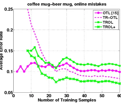
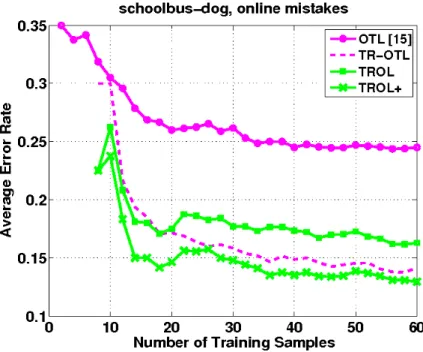
We assessed our proposed algorithms in the visual categories setting and evaluate the performance of our methods for online learning of visual categories. Following the setting proposed in [25], we used the Caltech-256 data set [15], for object category detection, considering a binary problem for each object class versus the background defined by the class clutter. By exploiting the taxonomy provided together with the images it is possible to set various transfer problems among differently related classes with one or multiple prior knowledge. For all the images we used the pre-computed SIFT features of [14]. The training set for each class consisted of 60 samples and the testing set for each class included 100 examples. Each set contains an equal number of positive (object class) and negative (background) data samples. We considered 10 random orderings of the samples for each class and we present the average results on these ten splits both in terms of the average error rate for the online methods and of the recognition rate produced by the current training solution on the test set. The training samples are always followed by a negative one and vice-versa and we can call such a sequential training data as concept drift. For all experiments we used the Gaussian kernel

K(x,x0) = exp(− 1

σ2kx−x

0_k2₎ _(5.1)

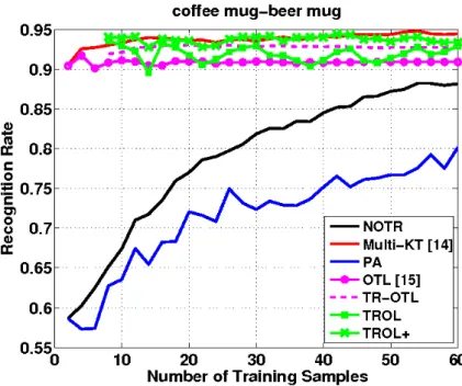
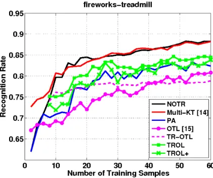
We fixed σ to the mean of the pairwise distances among the samples. We bench marked TROL and TROL+ against PA-algorithm trained on the target samples, Multi-KT (3.1.5) and OTL (3.2), where in case of multiple priors we considered the average of all the available models as source classifier.

This thesis is based on the work described in the following paper : T.Tomassi, F.Orabona, M.Kaboli, B.Caputo. Leveraging over prior knowledge for online learn-ing of visual categories submitted to BMVC2012 conference [27].

5.1.1 Baselines

To compare our experimental results we define the following baselines :

NOTR : This is a batch least square support vector machine (3.1.4) strategy corresponding to learn exploiting only the target samples and classify the unseen test data samples.

Multi-KT: This is the original batch transfer learning method presented in (3.1.5),[25].

PA: This is passive aggressive online learning strategy 2.2.2 on the available target samples for no transfer.

(45)

5.1. EXPERIMENTS

OTL : This is the online transfer learning method presented in (3.2), [31]. In case of multiple prior knowledges we consider the average of all the available mod-els as source classifier.

TR-OTL : This method considers as source knowledge for OTL the same Multi-KT output that we use as initialization in TROL.

M-OTL : This is our modified version of OTL able to assign a different weights to each prior knowledge in case of multiple sources, with the update rule defined in (4.18).

5.1.2 Initialization of Experiment

All the online techniques initialized with Multi-KT (3.1.5) use its output model learned over n= 6 training images, corresponding to three positive and three neg-ative samples. All the source models have been learned with LS-SVM (3.1.2). The value of the C parameter is chosen by cross validation on the sources and we used the same for the batch methods (Multi-KT and NOTR) applied on the new task. The C value for all the online methods is instead fixed to 1.

5.1.3 Single Source or Single prior knowledge

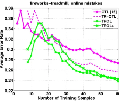
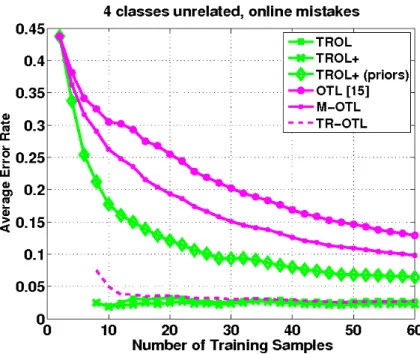
We ran a first group of experiments on couples of related and unrelated classes. The first ones are chosen inside the macro classes defined by the data set taxonomy, for instance, transportation-ground-motorized, food-containers, while the second ones are extracted randomly. For all the couples we consider one of the classes as target task and the other as a prior data. We repeat the experiments by terminating the role of the two classes finally, we report the obtained results as an average over each of the two classes.

Related Classes

Figure.(5.1) is the recognition rate which results on the test set and is plotted as a function of the number of training samples. It shows the experiments on the related