Statistical learning methods for multi-omics data integration in dimension reduction, supervised and unsupervised machine learning

(1)

STATISTICAL LEARNING METHODS FOR

MULTI-OMICS DATA INTEGRATION IN

DIMENSION REDUCTION, SUPERVISED AND

UNSUPERVISED MACHINE LEARNING

by

SungHwan Kim

M.S., Statistics, Korea University, South Korea, 2010

B.A., Education, Korea University, South Korea, 2007

Submitted to the Graduate Faculty of

the Department of Biostatistics of the

Graduate School of Public Health in partial fulfillment

of the requirements for the degree of

Doctor of Philosophy

University of Pittsburgh

2015

(2)

UNIVERSITY OF PITTSBURGH

DEPARTMENT OF BIOSTATISTICS OF THE GRADUATE SCHOOL OF PUBLIC HEALTH

This dissertation was presented by

SungHwan Kim

It was defended on April 20, 2015 and approved by

George C. Tseng, ScD, Professor, Department of Biostatistics, Graduate School of Public Health, University of Pittsburgh

YongSeok Park, PhD, Assistant Professor Department of Biostatistics, Graduate School of Public Health, University of Pittsburgh

Daniel E. Weeks, PhD, Professor, Department of Human Genetics, Graduate School of Public Health, University of Pittsburgh

Wei Chen, PhD, Assistant Professor, Department of Pediatrics, School of Medicine, University of Pittsburgh

Jing Lei, PhD, Assistant Professor, Department of Statistics, Carnegie Mellon University Dissertation Director: George C. Tseng, ScD, Professor, Department of Biostatistics,

(3)

STATISTICAL LEARNING METHODS FOR MULTI-OMICS DATA INTEGRATION IN DIMENSION REDUCTION, SUPERVISED AND

UNSUPERVISED MACHINE LEARNING

SungHwan Kim, PhD University of Pittsburgh, 2015

Abstract

Over the decades, many statistical learning techniques such as supervised learning, un-supervised learning, dimension reduction technique have played ground breaking roles for important tasks in biomedical research. More recently, multi-omics data integration analysis has become increasingly popular to answer to many intractable biomedical questions, to im-prove statistical power by exploiting large size samples and di↵erent types omics data, and to replicate individual experiments for validation. This dissertation covers the several analytic methods and frameworks to tackle with practical problems in multi-omics data integration analysis.

Supervised prediction rules have been widely applied to high-throughput omics data to predict disease diagnosis, prognosis or survival risk. The top scoring pair (TSP) algorithm is a supervised discriminant rule that applies a robust simple rank-based algorithm to iden-tify rank-altered gene pairs in case/control classes. TSP usually generates greatly reduced accuracy in inter-study prediction (i.e., the prediction model is established in the training study and applied to an independent test study). In the first part, we introduce a MetaTSP algorithm that combines multiple transcriptomic studies and generates a robust prediction model applicable to independent test studies.

One important objective of omics data analysis is clustering unlabeled patients in order to identify meaningful disease subtypes. In the second part, we propose a group structured

(4)

integrative clustering method to incorporate a sparse overlapping group lasso technique and a tight clustering via regularization to integrate inter-omics regulation flow, and to encourage outlier samples scattering away from tight clusters. We show by two real examples and simulated data that our proposed methods improve the existing integrative clustering in clustering accuracy, biological interpretation, and are able to generate coherent tight clusters. Principal componentanalysis(PCA)iscommonlyusedforprojectiontolow-dimensional spaceforvisualization. Inthethirdpart,weintroducetwometa-analysisframeworksofPCA (Meta-PCA)foranalyzingmultiplehigh-dimensionalstudiesincommonprincipalcomponent space. Theoretically,Meta-PCAspecializestoidentifymetaprincipalcomponent(Meta-PC) space; (1) by decomposing the sum of variances and (2) by minimizing the sum of squared cosines. Applications tovarious simulated data showsthat Meta-PCAs outstandingly iden-tify true principal component space, and retain robustness to noise features and outlier samples. We also propose sparse Meta-PCAs that penalize principal componentsin order to selectivelyaccommodatesignificantprincipalcomponentprojections. Withseveralsimulated and realdataapplications,we foundMeta-PCA efficienttodetectsignificanttranscriptomic features, and torecognize visual patternsfor multi-omics data sets.

In the future, the success of data integration analysis will play an important role in revealing the molecular and cellular process inside multiple data, and will facilitate disease subtype discovery and characterization that improve hypothesis generation towards pre-cision medicine, and potentially advance public healthresearch.

(5)

2.0 A TOP SCORING PAIR ALGORITHM IN META-ANALYTIC FRAME-WORK . . . 16

2.1 Introduction . . . 16

(6)

2.2.1 Top scoring pair algorithm (TSP) and kTSP . . . 18

2.2.2 Estimate K for kTSP . . . 21

2.2.3 Meta-kTSP algorithms . . . 22

2.2.4 Estimate K for Meta-kTSP . . . 24

2.3 Results . . . 24

2.3.1 Simulations. . . 24

2.3.2 Application to genomic data sets . . . 30

2.4 Discussion . . . 32

3.0 INTEGRATIVE MULTI-OMICS CLUSTERING FOR DISEASE SUB-TYPE DISCOVERY BY SPARSE OVERLAPPING GROUP LASSO AND TIGHT CLUSTERING . . . 40

3.2 Integrative clustering (iCluster) . . . 41

3.3 Group structured and tight integrative clustering . . . 42

3.3.1 Sparse overlapping group lasso . . . 42

3.3.2 Group structured integrative clustering (GS-iCluster) . . . 44

3.3.3 Group structured tight integrative clustering (GST-iCluster) . . . 47

3.3.4 Selection of penalization constant for GS-iCluster . . . 47

3.4 Applications . . . 49

3.4.1 Integration of mRNA, methylation and CNV using TCGA breast can-cer data . . . 50

3.4.2 Integration of mRNA and miRNA using TCGA breast data . . . 56

3.5 Simulation . . . 58

4.0 META-ANALYTIC FRAMEWORKS FOR PRINCIPAL COMPONENT ANALYSIS . . . 63

4.2 Methods. . . 66

4.2.1 Meta-PCA via sum of variance decomposition (SV) . . . 66

(7)

4.2.3 Variable selection of Meta-PCAs (Meta-sparsePCA) . . . 69

4.3 Simulation study . . . 70

4.3.1 True eigenvector detection of Meta-PCA . . . 70

4.3.2 Robustness of Meta-PCA . . . 74

4.4 Application to real data sets. . . 76

4.4.1 Spellman’s cell cycle data . . . 77

4.4.2 Prostate cancer data . . . 79

4.4.3 TCGA cancer data . . . 81

4.4.4 Mouse Metabolism Data . . . 82

4.6 Supplementary Materials . . . 85

4.6.1 Best choice of Meta-PC dimension . . . 85

4.6.2 Penalization constant for Meta-sparsePCA . . . 85

5.0 FUTURE WORKS AND CONCLUSION . . . 91

5.1 Meta-KTSP extended to multi-omics and multi-class problems. . . 91

5.2 GS-iCluster reflecting feature regulatory directions . . . 92

5.3 Conclusion . . . 92

(8)

LIST OF TABLES

1 The list of nine identified gene pairs of Average Meta-KTSP and the existing

breast cancer gene signatures. . . 30

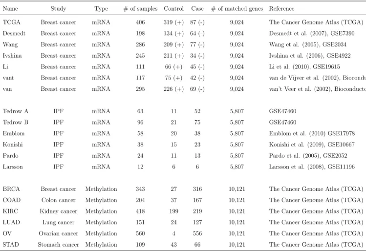
2 Shown are the brief descriptions of the nineteen microarray datasets of disease-related binary phenotypes (e.g., case and control or ER+/-). All datasets are publicly available. . . 33

3 Smoothing proximal gradient descent algorithm for structured likelihood func-tion.. . . 46

4 Analysis of three pathways over selected genes from both GS-iCluster and iCluster . . . 55

5 The number of selected features in modules with two or more features. . . 57

6 miRNAs set enrichment analysis of miRCancer database . . . 59

7 The algorithm of Meta-PCA via sum of variance decomposition (SV) . . . 67

8 The algorithm of Meta-PCA (Sum of squared cosine (SSC) maximization) . . 70

9 The four proposed methods of Meta-SparsePCAs for variable selection . . . . 71

10 The summary of four prostate cancer data. . . 79

11 Fisher discriminant scores of PC projections (prostate cancer data). . . 81

12 The summary of six TCGA methylation data. . . 82

13 Fisher discriminant scores of PC projections (TCGA pan-cancer data; Class lables: Tumor, Normal, Male and Female). . . 86

14 Fisher discriminant scores of PC projections (mouse metabolism data) . . . . 88

(9)

LIST OF FIGURES

1 Data structure of multiple genomic studies . . . 4

2 Overview of high-throughput data analysis. . . 6

3 Two major types of omics data integration (A) Horizontal omics meta-analysis to combine K transcriptomic datasets (B) Vertical omics integrative analysis to combine di↵erent omics data in a given cohort. . . 11

4 Two TSP examples from real data to show advantage of MetaTSP. X-axis and Y-axis refer to sample indices and gene expression levels, respectively. (A) Gene pair ITGAX/XBP1 has high TSP score (XBP1>ITGAX in controls but ITGAX>XBP1 in cases) in the training ‘Emblom’ study but fail to replicate in the testing ‘Konishi’ study as well as the other two Tedrow B and Pardo stud-ies. (B) Gene pair GPR160/COMP has high TSP scores (GPR160>COMP in controls and COMP>GPR160 in cases) in all three training studies ‘Emblom’, ‘Tedrow B’ and ‘Pardo’. The gene pair is successfully validated in the testing ‘Konishi’ study. . . 19

5 Results of inter-study prediction using four simulated data sets (A:µa= 1, B:

µa = 0.8; n11 =n21 = 100). Y-axis represents the average Youden index. The

bar plots indicate the standard error of estimated Youden index. . . 25

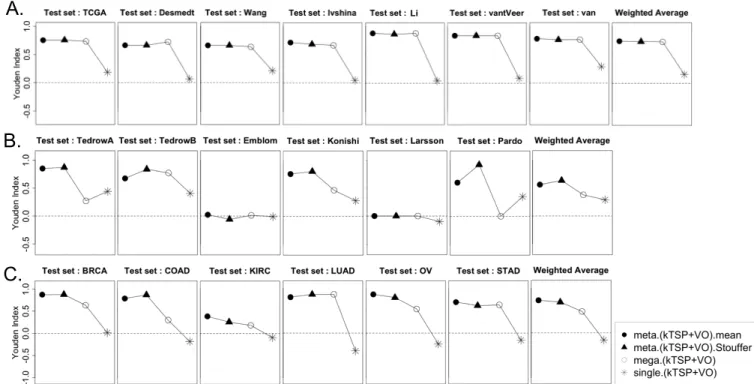
6 Three examples of Inter-study prediction with applications to real data sets (A. Breast Cancer: ER+ vs ER-, B. Idiopathic pulmonary fibrosis, B. Six di↵erents cancers in TCGA). Y-axis represents the average Youden index. . 28

(10)

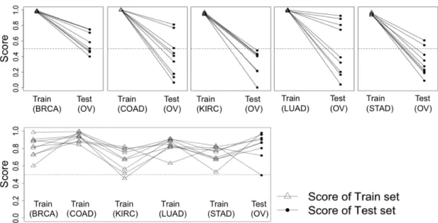
7 Comparison between single TSP scores and Meta-TSP scores using TCGA cancer data sets. The upper panels illustrate the scores of single study TSP to test data set (Ovarian; OV), whereas the bottom panel shows the Meta-TSP scores of multiple the train studies to test data set (Ovarian; OV). . . 29

8 Heatmap of the four simulated data. Genes encircled by red dotted line refer to correlated consensus genes. Study-specific genes are encircled by the blue dotted line. . . 34

9 Simulation results of the methods of TSP and MetaTSP family (µa= 1).. . . 35

10 Simulation results of the methods of TSP and MetaTSP family (µa= 0.8).. . 36

11 Performance comparisons of the methods of TSP and MetaTSP family using breast cancer mRNA data. . . 37

12 Performance comparisons of the methods of TSP and MetaTSP family using lung disease mRNA data. . . 38

13 Performance comparisons of the methods of TSP and MetaTSP family using TCGA pan cancer methylation data. . . 39

14 An example of penalization constant C implemented in sparse overlapping group lasso technique. . . 48

15 Heatmap of three omics (Gene, Methylation, and CNV) features selected via (A: Group structured / B: iCluster) integrative clustering. For ER and PR status, the pink and green colors represent ER-positive and ER-negative, re-spectively. For the rest, the pink color refers to Basal-like, Luminal A/B, and HER2 enriched, respectively. . . 51

16 Scatter plots of the top 12 feature modules that are negatively or positively mapped to the ordered mRNA features. Red, Blue, and Black colors rep-resent Methylation, CNV, and mRNA feature intensities, respectively. The values at the corner are correlations between two involving features, and each solid line represents a simple linear regression model of Methylation (Red) and CNV (Blue). Y-axis refers to expression levels, and X-axis samples ordered by mRNA expression. . . 52

(11)

17 Manhattan plots of pathway enrichment analysis (A: Result from GS-iCluster / B: Result from iCluster). . . 54

18 Heatmap of two omics (A:mRNA, Methylation and CNV / B:mRNA and miRNA) features selected via GST-iCluster. . . 56

19 A: Heatmap of two omics (mRNA and miRNA) features selected via Group structured integrative clustering, B:Heatmap of two omics (mRNA and miRNA) features selected via iCluster . . . 57

20 Performance comparisons between Group-structured integrative clustering and standard iCluster. . . 61

21 Examples of dimension reduction via PCA and Meta-PCA (SSC) over the four mouse metabolism omics data. The x-axis and y-axis refer to the first and second principal component projection. Red (WT), black (VLCAD), and blue (LCAD) colors represent wild-type, very longchain acyl-coenzyme A dehy-drogenase (VLCAD), and longchain acyl-coenzyme A dehydehy-drogenase (LCAD) deficiencies, respectively. Each figure (star, square, circle, and triangle) repre-sents each study label. . . 65

22 Geometrical illustrations for common principal component space (SSC). . . . 68

23 Performance comparisons (Meta-PCAs, PCA and JIVE) of the e↵ects on the number of studies for estimating true eigenvector. “SV”, “SSC” refer to Meta-PCA (SV) and Meta-Meta-PCA (SSC). “Single” represents standard Meta-PCA of each individual study (A:C = 0.1, B: C = 0.5, C and D: C= 1). . . 73

24 Robustness comparisons of Meta-PCA, JIVE and PCA to outliers and noises. The y-axis represents the averages of Fisher discriminant scores, and the x-axis the magnitude of cluster separation. The figure presents the two MetaPCA methods SV (dot), SSC (triangle), JIVE (circle) and standard PCA (Single, star) applied to each individual study. . . 75

25 Two dimensional PC projections of PCA, Meta-PCAs (SV, SSC), JIVE using four mRNA expression data sets of Spellman’s yeast cellcycle experiment. The numbers on the lines indicate time point during the two cell cycles. The first and second PC projection are on the x-axis and y-axis of each panel, respectively. 78

(12)

26 Two dimensional PC projections using four prostate cancer mRNA expression data sets; star (normal), square (primary tumor) and circle (metastasis tissues). The first and second PC projections are on the x-axis and y-axis, respectively. 80

27 Two dimensional PC projections using methylation expressions of six di↵erent cancers (TCGA) data; Tumor (square), Normal (dot), Male (black) and Female (grey). . . 83

28 Two dimensional PC projections using mRNA expressions of four mouse metabolo-ism data; WT (square), LCAD (dot) and VLCAD (star). . . 87

29 The example of scree plot to determine the optimal dimension reduction of Meta-PCA. . . 89

30 The example of scree plot to determine the penalization constant for Meta-sparsePCA. . . 90

(13)

1.0 INTRODUCTION

1.1 OVERVIEW OF HIGH-THROUGHPUT OMICS DATA

1.1.1 High-throughput data analysis

The system biological information flow is fundamentally rooted upon the central dogma paradigm from DNA to RNA, and RNA to Protein. This principle applies to all living creatures with exception of some simple organisms. DNA, encoding for genetic instructions, contains all necessary information for transcribing RNA transcripts, and hence functions as the structural sketch for cellular and bio-molecular mechanisms. The ground-breaking genome projects expedite deciphering genetic information of molecular organisms. Partic-ularly, whole genome sequencing has become a bifurcation toward the biomedical research history. Such advances in genomic technologies have spurred technological orchestration among various disciplines of biomedical, physiological, and bio-chemical sciences, and facili-tated the understanding of organismic functions, evolution and disease psychophysiology.

With the advance of modern bioinformatics, high-throughput technologies such as DNA microarrays, next generation sequencing (NGS) or mass spectrometry progressively produce abundant large genome-scale data with hundreds of thousands of features and large sample sizes. Over the past decades, genome profiling techniques have become viable at di↵er-ent levels of molecular cells and cellular organisms, including epigenome, transcriptome, metabolome, proteome, and interactome (Joyce et al.,2006). In addition, many other bioin-formatics technologies, such as proteomics assays and imaging techniques (e.g. fMRI and PET scan) have been actively applied to support the biomedical research community. Since each type of omics data has its unique characteristics, techniques that can accommodate

(14)

di↵erences of multiple types of omic data have been heavily sought beyond traditional bioin-formatics analysis. Recently, multi-omics data integration analysis has been highlighted by considering to elucidate inter-regulatory flows and whole bio-molecular systems. It has also revolutionized the understanding of the complex molecular biology process and disease devel-opments (Cancer Genome Atlas Research Network,2012). Furthermore, with the advances of hight-throughput technologies and rapid drop of the genomic experimental cost, generation of genomic data has been exponentially increased. Several large-scale data depositories have been constructed for public access such as Gene Expression Omnibus (GEO), ArrayExpress and Sequence Read Archive (SRA), and The Cancer Genome Atlas (TCGA). The emerging of large scale multi-omic data provides great opportunities for data integration analysis in the future.

1.1.2 High-throughput omics data technologies

1.1.2.1 Microarrays have been widely utilized in most of biological research domain and produced various real applications for translational research (?). Particularly, microar-ray data have been analyzed, together with computational algorithms and machine learning techniques, in applications for drug discovery, biomarker detection, pharmacology, toxicoge-nomics, prognostic testing, population genomics and disease subtype identifications. In the microarray technology, tens of thousands of microarray probes are immobilized on a solid support, such as a microscope glass slide or silicon chips. Labeled target sequences bind to probes for identifying unknown sequences. mRNA is reversely transcribed, amplified and hybridized to cDNA templates. Several levels of mRNA bound to di↵erent sites on the array for expression profiles of thousands of genes, and/or even the whole genome. The microar-ray technique can also be applied to detect single nucleotide polymorphisms (SNPs), copy number variation (CNVs), DNA methylation, and protein-DNA binding.

Since bulk microarray data sets have been generated, public access of those datasets have been required in hope of routinely storing and openly sharing of the data resources in the public domain. The National Center for Biotechnology Information (NCBI) has managed Gene Expression Omnibus (GEO), where a multitude of gene expression data

(15)

sets are available. The Cancer Genome Atlas (TCGA, https://tcga-data.nci.nih.gov/tcga/) provides large-scale microarray datasets that can be downloaded via a public access. Up to date, TCGA has accumulated over 600 miroarray samples that are clinically annotated to primary breast cancer specimens. In this dissertation, several public microarray datasets are used to demonstrate our novel bioinformatics analysis methods such as robust prediction rules, coherent disease subtype identification, feature discovery, and dimension reduction for data visualization.

1.1.2.2 Next-generation sequencing (NGS) has been introduced in recent years, and mostly used in many biomedical applications (e.g., mutation discovery, meta-genomics, defin-ing DNA-protein interactions, noncoddefin-ing RNAs, and de-novo assembly of transcriptomic se-quences, (Mardis,2008). Next-generation sequencing is so-called ultra deep high-throughput that processes millions of sequence reads simultaneously. The workflow is to bind specific adapter oligos to both ends of each DNA fragment and then sequence the DNA fragments. Next-generation sequencers can generate short sequencing reads while read lengths can vary depending on user preference, technologies or platforms (e.g., Illumina1, SOLiD2, Roche). The generated short sequencing reads are aligned to a reference genome or transcriptome to quantify the expression levels of genes or transcripts by counting mapped short reads.

RNA-Seq is the most popular next-generation sequencing technology to quantify gene expression. RNA-Seq is an efficient way to produce gene-expression profiles, transcriptional structures of genes, and post-transcriptional modifications. Compared to the microarray technology, RNA-Seq has quite a few better properties such as high resolution, novel exons and genes detection, higher specificity and sensitivity with low background noise, no need for reference sequence, distinguishing isoforms and allelic expression (Wang et al., 2009), and accurately measuring the amounts of transcripts and their isoforms (alternatively spliced transcripts from the same gene). RNA-Seq can be flexibly extended to di↵erent types of analyses, for example, single nucleotide polymorphism discovery, alternative transcript iden-tification, and gene expression profiling. TCGA projects also include thousands of primary tumor samples from more than 30 di↵erent tumor types in order to study underlying mech-anism of malignant transformation and progression (http://tcga-data.nci.nih.gov/tcga).

(16)

!_!!(!)!!!_!"(!)!!!!!!!!∙∙∙!!!!!!!!_!_!(!) (!) _!_! !_!"(!)!!!_!!(!)!!!!!!!!∙∙∙!!!!!!!!_!(!_!()!)! !_!"(!)!!!_!"(!)!!!!!!!!∙∙∙!!!!!!!!_!_!(!) (!) ! !!!!!!!!!∙!!!!!!!!!!!!!!!!!!!!!!!!!!!!!!!!!!!!!!!!∙!!!!!!!!! !!!!!!!!!∙!!!!!!!!!!!!!!!!!!!!!!!!!!!!!!!!!!!!!!!!∙!!! !!!!!!!!!∙!!!!!!!!!!!!!!!!!!!!!!!!!!!!!!!!!!!!!!!!∙!!! !!!!!!!!!∙!!!!!!!!!!!!!!!!!!!!!!!!!!!!!!!!!!!!!!!!∙!!! !!!!!!!!!∙!!!!!!!!!!!!!!!!!!!!!!!!!!!!!!!!!!!!!!!!∙!!! ! !_!(!_!)!!!_!(!_!)!!!!!!!!∙∙∙!!!!!!!!_!_!(!) (!) ! ! 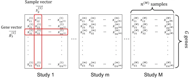Gene$vector$ !!_!(!)$ !_!!(!)!!!_!"(!)!!!!!!!!∙∙∙!!!!!!!!_!_!(!) (!) _!_! !_!"(!)!!!_!!(!)!!!!!!!!∙∙∙!!!!!!!!_!(!_!()!)! !_!"(!)!!!_!"(!)!!!!!!!!∙∙∙!!!!!!!!_!_!(!) (!) ! !!!!!!!!!∙!!!!!!!!!!!!!!!!!!!!!!!!!!!!!!!!!!!!!!!!∙!!!!!!!!! !!!!!!!!!∙!!!!!!!!!!!!!!!!!!!!!!!!!!!!!!!!!!!!!!!!∙!!! !!!!!!!!!∙!!!!!!!!!!!!!!!!!!!!!!!!!!!!!!!!!!!!!!!!∙!!! !!!!!!!!!∙!!!!!!!!!!!!!!!!!!!!!!!!!!!!!!!!!!!!!!!!∙!!! !!!!!!!!!∙!!!!!!!!!!!!!!!!!!!!!!!!!!!!!!!!!!!!!!!!∙!!! ! !_!(!_!)!!!_!(!_!)!!!!!!!!∙∙∙!!!!!!!!_!_!(!) (!) ! ! !_!!(!)!!!_!"(!)!!!!!!!!∙∙∙!!!!!!!!_!_!(!) (!) _!_! !_!"(!)!!!_!!(!)!!!!!!!!∙∙∙!!!!!!!!_!(!_!)(!)! !_!"(!)!!!_!"(!)!!!!!!!!∙∙∙!!!!!!!!_!_!(!) (!) ! !!!!!!!!!∙!!!!!!!!!!!!!!!!!!!!!!!!!!!!!!!!!!!!!!!!∙!!!!!!!!! !!!!!!!!!∙!!!!!!!!!!!!!!!!!!!!!!!!!!!!!!!!!!!!!!!!∙!!! !!!!!!!!!∙!!!!!!!!!!!!!!!!!!!!!!!!!!!!!!!!!!!!!!!!∙!!! !!!!!!!!!∙!!!!!!!!!!!!!!!!!!!!!!!!!!!!!!!!!!!!!!!!∙!!! !!!!!!!!!∙!!!!!!!!!!!!!!!!!!!!!!!!!!!!!!!!!!!!!!!!∙!!! ! !_!(!_!)!!!_!(!_!)!!!!!!!!∙∙∙!!!!!!!!_!_!(!) (!) ! ! Sample'vector' !!_!(!)'

…

Study 1

Study m

Study M

!(!)_!samples!

Figure 1: Data structure of multiple genomic studies

1.1.3 Data structure of omics study

In genomic data analysis, large-scale genomic data are generated under various conditions for di↵erent tissue samples. As shown in Figure 1, the data after proper pre-processing are in an expression matrix D=_{x(_ijm)_} (1_i_G,1_j _n(m)_,₁__m __M_{), where the rows} refer to expression features, the columns represent sample profiles, andx(_ijm)is the expression level for gene i in samplej of study m. !gi(m) ={x(im1), . . . , x

(m)

in(m)} is theith gene vector that

contains expression levels across all samples of study m. !sj(m) ={x(1mj);. . . , x

(m)

Gj } is the jth

sample vector of expression levels across all gene features in study m. In microarray data,

x(_ijm) is a log2 transformed of raw intensity or an intensity ratio as continuous values. For RNA-Seq data, x(_ijm) is the read count of gene iof subjectj in studym. In this dissertation, we use these notations and the dataset structure unless explicitly described.

(17)

1.2 MACHINE LEARNING ANALYSIS ON HIGH-THROUGHPUT OMICS DATA

1.2.1 Major aims of statistical analysis in bioinformatics

The analyses of high-throughput data can be classified into two based on its major objectives. The first aim is to decipher underlying biological or disease development system through var-ious omics data from di↵erent patient cohorts or/and varvar-ious treatments. Exploitative and analytic methods such as di↵erential expression (DE) analysis, clustering analysis, pathway analysis, and network analysis (Hawkins et al., 2010; Quackenbush, 2001) have played cru-cial roles in the identification of relations between bio-molecular units and clinical phenotype patterns (e.g., candidate biomarker detection, disease subtype identification and associated biological pathways) (Figure 2). This analytic trend has also revolutionized the target drug development, preventive disease procedures (Zografos et al., 2013) that will ultimately lead to “translational medicine” (Winslow et al.,2012). For example, breast cancer developments has diverse patterns that depend on expressed marker genes related to Estrogen Receptor (ER)-positive or negative. Accurate biomarker detection closely links to the success of rele-vant clinical treatments and/or radio- or chemotherapy.

The second objective is to identify novel biomarker classifiers for clinical trial design and decision theory in many biomedical applications (Baek et al.,2009). The advent of prediction rules applicable to high-throughput omics data facilitates novel translational products such as disease diagnosis, prognosis prediction, treatment selection, preventative intervention, and precision medicine. However, high-throughput genomic, proteomic and metabolomic data brings new challenges in constructing robust prediction models. Model building with e↵ective feature selection closely links to success in the development of a biomarker classifier. For this reason, the e↵ort to detect biomarkers of disease development (translational products in the aim above) can closely related to developing accurate and feasible prediction models (Figure 2).

In Chapter 2, we propose “meta top scoring pairs (Meta-TSP)”, a robust prediction model using the rank-order of paired genes. Meta-TSP can successfully function as a disease

(18)

prediction model. In Chapter 3, we develop “group structured tight integrative clustering (GST-iCluster)”. We show that GST-iCluster can efficiently identify biologically relevant genes related to disease development mechanisms, and discover coherent disease subtypes. We expect these machine learning methods will significantly contribute to the community of the high-throughput omic data analysis.

High throughput omics data (e.g. microarray, NGS, proteomics)

•  Understand disease mechanisms •  Differential expression analysis •  Cluster analysis •  Pathway enrichment analysis •  Network analysis •  Biomarkers of disease development •  Targeted drug development •  Preventive treatment •  Develop prediction model •  Discriminant rules by machine learning •  Decision model

•  Clinical trial design

•  Disease diagnosis, prognosis, treatment decision •  Precision medicine •  Disease prevention Data source Goals Bioinformatics techniques Translational products

(19)

1.2.2 Unsupervised learning on omics data

Unsupervised machine learning, aka clustering analysis, is a set of methods that do not rely on class label information, and separate samples into clusters under a predefined distance measure. By nature of unsupervised learning, it is intractable to evaluate its statistical prop-erty and performance due to the absence of so-called “gold standard”. When performing clustering analysis, a distance or dissimilarity matrix measures the degree of closeness or sep-aration of each pair of observations, and thereby a clustering algorithm can assign samples in proximity to each cluster. Many classical algorithms such as hierarchical clustering (Defays,

1977), K-means (Hartigan et al., 1979), self-organizing maps (Kohonen, 1982), Gaussian mixture model-based clustering (Banfield et al., 1993) and Bayesian clustering (Laua et al.,

2007) have been developed. In addition, to control separation degrees of estimated clusters, a few cutting-edge methods have been proposed such as tight clustering (Tseng and Wong,

2005), penalized K-means (Tseng, 2007), and consensus clustering (Monti et al.,2003). Consider a gene expression matrix of p genes and n samples. The data matrix can be viewed from row-wise (clustering genes) or column-wise (clustering samples) perspectives. When performing gene clustering, it is believed that highly correlated genes have a high chance of belonging to the same co-regulated systems and similar biological functions. Such gene cluster analysis generates gene modules that reveals relevant biological functions and evidences. In contrast, the problem of disease subtype discovery (clustering samples) has also been received wide attention. The purpose of subtype discovery is to cluster samples based on expression profiles in hope of identifying patient clusters with biologically (e.g. di↵erent pathway activation and disease progression mechanisms) and clinically (e.g. di↵erent drug response or survival) meaningful disease subtypes. For example, breast cancer was once thought as one type of disease. However, the well-known paper from Perous lab (Perou et al.,

2010) applied hierarchical clustering in their microarray dataset and successfully identified five molecular breast cancer subtypes (Luminal A, Luminal B, Basal, Her2, and Normal-like) and demonstrated their biological and clinical relevance. This finding of novel disease subtypes will eventually become the fundamental basis for precision medicine.

(20)

1.2.3 Supervised discriminant analyses on omics data

Supervised machine learning has contributed to the advance of biomedical and clinical appli-cations. In general, the task is to learn a classification model from training high-throughput data and predict the disease status or prognosis for incoming new patients. For instance, MammaPrint (Cardoso et al., 2007) established via supervised learning is a diagnostic tool to assess the metastatic risk of breast tumor based on the Amsterdam 70-gene breast cancer signature. MammaPrint measures a dichotomous risk using microarray profiles and samples from lymph node-negative breast cancers.

Here we introduce the generic data structure for supervised machine learning. Let G

dimensional random vector !X = (!g1, . . . ,g!G) be the input data of population as covariates

(e.g. the gene expression of G genes) and a random variable Y of values on {1,2, . . . , K} as the class labels. In biomedical research, X can be high-throughput data that contain G

features of clinical variables, gene expression levels, miRNA expression levels, protein ex-pression levels, methylation intensities, SNPs/mutations. Y represents labels for di↵erent groups such as “disease vs control”, “metastatic vs non-metastatic”, “short patient survival vs long patient survival”, “drug respondents vs non-respondents” or “multiple disease sub-types”. The observed data as a whole comprisenpatients: D= ((y1,!s1), . . . ,(yn,!sn)) where

(yj,!sj) ⇠ (Y,!X) for 1  j  n. Using supervised learning techniques, a model is learned

from the observed data D (including label information), and predicts new labels for future patients.

When applying machine learning techniques, it is essential to understand the motivations and details of each algorithm (e.g. data distribution assumption) to achieve accurate and interpretable results. The true distribution of data is typically unknown and is impossible to precisely estimate under high-dimensional settings due to “Curse of dimensionality” (refer to Section 1.3) . This problem has led to development of various machine learning methods based on di↵erent assumptions and types of data structure. To analyze high-throughput data, many popular machine learning methods have been proposed and applied, such as logistic regression, linear (quadratic) discriminant analysis, classification and regression tree (CART), random forest and support vector machines. There are also many fundamental

(21)

issues for better fitting machine learning models, e.g. cross-validation, feature selection and avoiding overfitting.

1.3 DIMENSION REDUCTION ON HIGH-THROUGHPUT OMICS DATA

With the advances in technology, high-dimensional data are now commonly generated in a wide range of research fields including genomics, signal processing, and financial risk man-agement. The data analysis methods to deal with high dimensionality have been received increasing attentions as high-dimensional and large size data are accumulated over the years. The term of “Curse of dimensionality” introduced by Richard Bellman (Richard et al.,1957) refers to problems that occur under high-dimension of state variables in optimization prob-lems (e.g. the computing complexity increases exponentially as the dimension increases). As a solution to this, he proposed a dynamic programming method for particular optimization problems. When fitting statistical models, the “curse of dimensionality” causes estimation to converge at a very slow rate. For example, the required sample sizes are only 4 and 19 for one or two dimensional space, whereas the required sample size rises to 842,000 if the dimension increases to 10. Another example is “concentration of measure” that influences the shape of a standard multivariate (d-dimensional) normal distribution. When d=1 or 2, the density concentrates to the origin, but when d is large, the distribution is concentrated on a d-dimensional sphere/shell with radius equalspd.

To circumvent high dimensionality problems, many dimension reduction techniques have been developed (e.g. Principal component analysis (PCA), multidimensional scaling (MDS), non-negative matrix factorization (NMF), etc.). In particular, the dimension reduction is suitable for high-throughput genomic data analysis, in which the signals of interest to dif-ferentiate groups tend to be in lower dimension subspace. Nevertheless, there are still many practical challenges of PCA method to deal with high-dimensional data. For example, noise features contained in most of large-scale microarray data often cause potential failure of dimension reduction (Hubert et al., 2005).

(22)

1.3.1 Principal component analysis (PCA)

Principal component analysis (PCA) has been one of the most popular data-processing and dimension reduction technique in multivariate analysis. It is particularly suitable to discover low-dimensional signals for high-dimensional data. In the setting of small-p and large-n, the estimated principal components of the covariance matrix are shown to be consistent as the sample size n increases when p fixed. For high-throughput data analysis, PCA has been applied to gene expression data (Alter et al., 2000). For example, the “gene shaving” technique (Hastie et al., 2000) uses PCA to cluster highly variable and coherent genes in microarray datasets. In spite of its advantages, PCA has several fundamental flaws.

Several experimental studies (Baik et al., 2006) show that the sample principal com-ponent is inconsistent with the principal comcom-ponent of whole population. For example, the high-dimensional setting of large-p and small-n causes very poor estimates. In addi-tion, sample principal eigenvectors generally have nonzero loading values for each coordinate component. This drawback results in low interpretability as the dimension p increases. To overcome this issue, we introduce a meta analytic framework for principal components (Meta-PCA) in Chapter 4. Meta-PCA is designed to discover the best common eigenvector space, and is less sensitive to the e↵ect of noise samples and features than single PCA method.

1.3.2 Regularized principal component analysis (Sparse PCA)

Sparse PCA is designed to overcome the aforementioned shortcomings of PCA, especially, the variable selection problem in high dimensional eigenvectors. In theory, PCA holds two bene-ficial properties: (1) the leading principal components minimize information loss (maximized variability);(2) Principal components are projected into perpendicular subspaces. However, small but non-zero loadings from many features in eigenvectors often act as a major barrier to interpret estimated principal components. One potential way to increase the interpretabil-ity of principal component (PC) is to apply regularization (i.e., penalization) over leading eigenvector components. This approach is commonly called “sparse PCA”, and various sparse PCA methods have been proposed in the literature (Hoyle et al., 2004; dAspremont et al., 2007; Journ ee et al., 2010; Shen et al., 2008; Ulfarsson et al., 2008; Jolli↵e et al.,

(23)

2003; Witten et al., 2009; Zou et al., 2006). Jolli↵e et al. (2003) introduced SCoTLASS to estimate principal components with possible zero loadings. Zou et al. (2006) proposed sparse PCA (SPCA) based on a regression-type optimization via the elastic net incorporat-ing the regression technique. Similar to SPCA, Witten et al. (2009) developed sparsePCA that exploits the penalized matrix decomposition (PMD) using SVD approximated matrix to minimize errors to the original observed matrix. In Chapter 5, we develop several sparse Meta-PCAs to improve the proposed Meta-PCA’s interpretability. Various numerical ex-amples have shown the sparse Meta-PCAs outperform Meta-PCA in favor of efficient and distinctive visualization in low dimension space.

1.4 MULTI-OMICS DATA INTEGRATION ANALYSIS

Figure 3: Two major types of omics data integration (A) Horizontal omics meta-analysis to combine K transcriptomic datasets (B) Vertical omics integrative analysis to combine di↵erent omics data in a given cohort.

(24)

1.4.1 Horizontal omics data integration (Meta-analysis)

In the past two decades, high-throughput experimental techniques have revolutionized biomed-ical research with large genome-scale data. The fruitful successes of this research are paving the way towards better drug targets and precision medicine. Such “big” datasets are rou-tinely generated now that the cost has been greatly decreased. As a result, abundant datasets are available in the public domain. For example, as of 9/16/2014, GEO contains 1,234,880 samples and SRA has>2,826 terabases of sequencing data. E↵ective integrative methods are urgently required to decipher the biological information inside these data, leading to a bet-ter understanding of disease mechanisms. Omics integrative methods are commonly divided into two major categories. Due to high experimental cost, and/or limitation of clinical tissue access, individual labs usually generate omics datasets with small to moderate sample sizes (e.g. n=40-100). Statistical power and reproducibility of such small studies has long been a concern in this field (Simon et al.,2003;Simon, 2005;Domany, 2014). An increasingly pop-ular solution is to search the literature, seek similar datasets (of similar design and biological hypothesis) and perform data integration. In this context, the analytic questions and meth-ods are analogous to traditional meta-analysis (Ramasamy et al., 2008; Tseng et al., 2012). Since the microarray boom of the late 90s, a convention has been developed in which genes on the rows and samples on the columns. As a result, multi-study data integration is often called “horizontal omics meta-analysis” since datasets are laid out horizontally (Figure3A). The horizontal meta-analysis methods can conceptually be applied to other types of omics data, such as GWAS, mRNA expression, methylation, miRNA, copy number variation and protein expression. In particular, horizontal meta-analysis methods are useful and practical for individual labs mostly generating data of moderate sample size. Successful development of horizontal meta-analysis methods for subtype discovery and characterization can greatly enhance knowledge of finding and generating hypotheses towards precision medicine. In this dissertation, we introduce two methods on horizontal data integration analysis. In Chapter 2, we introduce “meta top scoring pairs (Meta-TSP)”, a robust prediction model of paired genes. TSP integrates multiple studies when the prediction model is fitted, so Meta-TSP generates high accuracy especially in inter-study prediction. In Chapter 4, we propose

(25)

a meta-analytic framework for principal component analysis (Meta-PCA). Single PCA study tends to be sensitive to the e↵ects of noise samples and features in high-dimensional data. On the contrary, Meta-PCA aims to form common eigenvector space that can capture varia-tions of multiple studies in parallel. Due to nature of common eigenvector space, Meta-PCA is robust to noise features and outlier samples.

1.4.2 Vertical omics data integration

In contrast to horizontal meta-analysis, many large consortia (e.g. the Cancer Genome Atlas (TCGA) and the Lung Genomics Research Consortium (LGRC)) have started to generate multiple di↵erent types of -omics data using samples in a single cohort, including SNP genotyping, mutation, copy number variation, mRNA expression, miRNA expression and protein expression. The integration of the multi-omics data for understanding the inter-omics interaction mechanisms is challenging in statistical problem. The datasets are aligned vertically (Figure 3B) and thus, the integration of such multi-omics data is called “vertical omics integrative analysis”. While integration of multiple omics data sources on the same cohort provides great insight into the molecular and cellular processes of the disease and has become popular, the problem brings new analytical challenges and it is in need to develop of statistical methods in this field.

Similar to traditional microarray data analysis, vertical omics integration can target on the following biological objectives: (i) candidate marker detection (Wang et al., 2008); (ii) gene set or pathway analysis (Hu et al.,2014); (iii) dimension reduction (Lock et al.,2013A;

Li et al., 2012; Zhang et al., 2011); (iv) classification (Setty et al., 2014); and finally (v) clustering analysis. Using multi-omics data sources, several methods for disease subtype discovery using vertical omics integration have been proposed. Rey and Roth (2012) in-troduced a copula mixture model for dependency-seeking clustering of multi-omics data.

Lock et al. (2013B) proposed a Bayesian consensus clustering to account for consensus and source-specific information in the cluster formation.

Shen et al. (2009, 2013) developed an integrative clustering approach (iCluster) via a Gaussian latent regression model. iCluster has several advantages that brought it

(26)

pop-ularity in many, particularly cancer, applications. Multi-omics integrative clustering has the focus to identify disease subtypes. For n subjects, suppose we have M di↵erent omics datasets. Let X(m) _{be the} _mth _{dataset with} _p

m features, where each column of X(m)

con-sists of mean-centered features of n subjects (1 _ m _ M). The combined dataset is

X =⇣X(1)T

, X(2)T

, . . . , X(M)T⌘T

, whereX is aPM_m₌₁p(m)_⇥_n_{matrix, and} _X(m) _{is a}_p(m)_⇥_n matrix. The joint latent regression model is

X(m) =B(m)Z+E(m) for 1_m_M,

where Z is a `_⇥n matrix whose rows are latent variables and columns are samples. The matrix B(m) _{is used to control the degree of relation between feature intensities and} la-tent variables (usually l << p(m)_,₈_m_{). To achieve the sparse estimation of} _B(m)_{, the} expectation-maximization (EM) algorithm (Dempster et al., 1977) is applied to estimate

ˆ

B and ˆ, together with a L1-lasso penalty (Tibshirani, 1996). Once we estimate the latent variable matrix Z, the standard k-means clustering is applied toZ with respect to samples to produce the integrative clusters.

1.5 OVERVIEW OF THE DISSERTATION

This dissertation covers three major data integration analyses: (1) robust prediction in a meta-analytic framework (horizontal integration); (2) coherent and tight integrative cluster-ing specialized in feature gene discovery (vertical integration); (3) meta-analytic framework of dimension reduction for visualization (horizontal integration). In Chapter 2, we introduce a MetaTSP algorithm that combines multiple transcriptomic studies and generates a robust prediction model applicable to independent test studies. The top scoring pair (TSP) algo-rithm is a supervised discriminant rule by applying a robust simple rank-based algoalgo-rithm. TSP exhaustively explores rank-altered gene pairs in case/control classes but often su↵ers from low accuracy in inter-study prediction (i.e. the prediction model is established in the training study and applied to an independent test study). With comprehensive applications and simulated data, the performance of MetaTSP is shown to outperform single study TSP.

(27)

In Chapter 3, we propose a group structured iCluster together with a sparse overlapping group lasso technique via regularization to incorporate information of inter-omics regulation flow, and also applying a tight clustering concept to form tight clusters by scattering outlier samples away. This integrative clustering (unsupervised) method can identify meaningful disease subtypes and biologically associated gene modules. We show by two real examples and simulated data that our proposed methods improve the original iCluster in clustering ac-curacy, biological interpretation, and are able to generate coherent tight clusters. In Chapter 4, we introduce two meta-analysis frameworks of PCA (Meta PCA) for analyzing multiple high-dimensional studies in common principal component space. Meta PCA aims to identify the best common PC space. Applications to various simulated data show that Meta PCA is able to find the true principal component space, and retains robustness on noise features and outlier samples. In Chapter 5, we further propose several sparse Meta PCA methods that can regularize principal components, and facilitate feature identifications and visual pattern recognition for multiple omics datasets.

(28)

2.0 METAKTSP: A META-ANALYTIC TOP SCORING PAIR METHOD FOR ROBUST CROSS-STUDY VALIDATION OF OMICS PREDICTION

ANALYSIS

2.1 INTRODUCTION

High-throughput experimental techniques, including microarray and massively parallel se-quencing, have been widely applied to discover underlying biological processes and to pre-dict the multi-causes of complex diseases (e.g., cancer diagnosis, (Ramaswamy et al.,2001), prognosis (van de Vijver et al., 2002), and therapeutic outcomes (Ma et al., 2004)). The associated data analysis has brought new statistical and bioinformatics challenges and many new methods have been developed in the past 15 years. In particular, methods for classifi-cation and prediction analysis (a.k.a. supervised machine learning) are probably the most relevant tools towards translational and clinical applications. Take breast cancer as an ex-ample, many expression-based biomarker panels have been developed (e.g. MammaPrint (van ’t Veeret al.,2002), Oncotype DX (Paiket al.,2004), Breast Cancer Index BCI (Zhang

et al., 2013) and PAM50 (Parker et al., 2009)) for classification/prediction of survival, re-currence, drug response and disease subtype. Reproducibility analysis of these markers and classification models has been a major concern and has drawn significant attention to ensure clinical applicability of these panels (Garrett-Mayer et al., 2008; Kuo et al., 2006; MAQC Consortium et al., 2006; Mitchell et al., 2004; Sato et al., 2009). Many papers have focused on normalization, reproducibility of marker detection, inter-lab or inter-platform correlation concordance. For direct clinical utilities, more attention have shifted towards cross-study situation or inter-study prediction (i.e. a prediction model is established in one study and validated independently in a test study (Xu et al., 2008; Chenget al., 2009; Mi et al., 2010;

(29)

Bernau et al., 2014)). Such an issue is critical for translating models from transcriptomic studies into a practical clinical tool. For example, the training cohort may have utilized an old A↵ymetrix U133 platform. A biomarker panel and a model are constructed and a test study from a di↵erent medical center using an RNA-seq platform is available. A successful machine learning model should retain high prediction accuracy in such inter-lab and inter-platform validation. We note that many normalization methods have been developed to adjust for systematic biases across studies, including distance weighted discrimination (DWD, (Benito

et al., 2004)), cross-platform normalization (XPN, (Shabalin et al., 2008)) and Knorm cor-relation (Tenget al.,2007). But the normalization performance largely depends on whether the observed data structure fits the model assumptions. In most applications, researchers have often applied meta-analysis methods instead of normalization and data merging (Tseng

et al.,2012). Similarly, we will not consider normalization and data merging approach (a.k.a. mega-analysis).

In addition to the issue of cross-study validation, selection of a robust and accurate ma-chine learning method is also critical. In the literature, many supervised mama-chine learning methods have been proposed and applied to high-throughput experimental data. For ex-ample, the CMA package allows easy implementation of 21 popular classification methods such as linear or quadratic discriminant analysis, lasso, elastic net, support vector machines, random forest, PAM, etc (Slawskiet al., 2008). Most of these parametric and model-based methods potentially can su↵er from heterogeneity across platforms and limit the feasibility and reproducibility in the cross-study validation. In addition to these popular methods, the top scoring pair (TSP) method (Geman et al., 2004; Tan et al., 2005; Afsari et al., 2014) is a straightforward prediction rule utilizing building blocks of rank-altered gene pairs in case and control comparison (see Section 2.1 for more details). The method is rank-based without any model parameter. It is invariant to monotone data transformation that relieves from normalization necessity, and the feature selection and the model are more transparent for biological interpretation. Although TSP and its variant are robust methods that do not require normalization in cross-study validation, we have found that some of the selected TSPs from the training study may not reproduce in the test study and appear to be false positives.

(30)

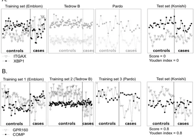
Here we consider four Idiopathic pulmonary fibrosis(IPF) studies (see Table 2). Figure 1A illustrates the expression levels of a good TSP gene pair, CBS and MOXD1, identified from the first IPF training study Emblom XBP1 is more over-expressed than ITGAX in control samples but under-expressed in cases. If we use this TSP to validate in the test study Konishi, we find that XBP1 is over-expressed than ITGAX in both cases and controls and we obtain 0% sensitivity and 100% specificity (i.e. Youden index = sensitivity + specificity -1 = 0). We find similar poor performance in two other studies Tedrow B and Pardo, showing that the TSP is likely a false positive. In Figure 1B, GPR160 is over-expressed than COMP in controls and under-expressed in cases for all three studies Emblom, Tedrow B and Pardo. It is a more reliable TSP across three studies and conceptually is less likely a false positive. Indeed, the cross-study validation in Konishi shows good performance with 80% Youden index. The two real examples in Figure 1 argue the potential of a meta-analytic approach by combining multiple training transcritomic studies to identify reliable TSPs so the resulting model has enhanced cross-study validation performance.

2.2 METHODS

2.2.1 Top scoring pair algorithm (TSP) and kTSP

The original TSP algorithm was first proposed by Geman et al. (2004). Denote by data matrix X ={xgn} the gene expression intensity of gene g (1  g  G) in sample n (1 n

 N) and yn the class label of sample n. Particularly, we consider yn2{0,1}, representing

controls and cases for binary classification. For any gene pairi and j (1 i, j  G), define the conditional ordering probability scoreTij(C) =P r(Xi< Xj|Y =C) forC2{0,1}, where

XiandXj are gene expression intensities of geneiandj. Intuitively,Tij(0) is the probability

in controls that genej has larger expression intensity than that of geneiand similarlyTij(1)

is for cases. Given observed expression profile data matrix X, the probability scores can be estimated as ˆTij(C) = ⇣ PN_n₌₁I(xin < xjn)·I(yn =C)⌘ ⇣ P_nN₌₁I(yn =C)

⌘

, where I(_·) is an indicator function that is one if the statement inside the parenthesis is true and zero

(31)

oth-A.!

B.!

Figure 4: Two TSP examples from real data to show advantage of MetaTSP. X-axis and Y-axis refer to sample indices and gene expression levels, respectively. (A) Gene pair IT-GAX/XBP1 has high TSP score (XBP1>ITGAX in controls but ITGAX>XBP1 in cases) in the training ‘Emblom’ study but fail to replicate in the testing ‘Konishi’ study as well as the other two Tedrow B and Pardo studies. (B) Gene pair GPR160/COMP has high TSP scores (GPR160>COMP in controls and COMP>GPR160 in cases) in all three training studies ‘Emblom’, ‘Tedrow B’ and ‘Pardo’. The gene pair is successfully validated in the testing ‘Konishi’ study.

(32)

erwise. The discriminant score of the gene pair is defined asSij = ˆTij(1) Tˆij(0). Note that

1_Sij 1 always holds. WhenSij = 1, expression of genej is always greater than that of

geneiin cases and expression of gene j is always smaller than that in geneiamong controls. As a result, the ordering of gene iand gene j expression is predictive to the class label. On the contrary, if Sij = 1, gene j always has smaller expression than gene i in cases and the

relation is reversed in controls. In summary, the absolute value of Sij reflects the predictive

value of the gene pair. The TSP algorithm seeks the best gene pair (i⇤, j⇤) = arg maxi6=j|Sij|

as the classifier. When multiple gene pairs give the same highest absolute score, the best pair that gives the largest di↵erential magnitudeDij is chosen, where Dij =|dij(1) dij(0)|

and dij(C) = ⇣ P_nN₌₁(xin xjn)·I(yn = C)⌘ ⇣ P_nN₌₁I(yn = C)

⌘

. When a new test sam-ple!x(test)= x(1test),· · ·, x

(test)

G is entered in the future, the class prediction is determined by

ˆ Ci⇤_j⇤(!x(test)) = 8 > < > : 1, if Si⇤j⇤· ⇣ x(_i⇤test) x(jtest⇤ ) ⌘ 0 0, if Si⇤_j⇤· ⇣ x(_i⇤test) x(_jtest⇤ ) ⌘ >0

TSP classifier above is based on only one top scoring pair (two genes) and so the method can be very sensitive to slight noise perturbations (Geman et al., 2004). To circumvent this issue, Tan et al. (2005) introduced kTSP to combine multiple TSPs for a more stable algorithm. The method identified the sorted TSPs similar to above. Instead of choosing only the best TSP, it selected the topK (whereK is a parameter to be tuned) TSPs to construct the model. The TSPs were selected from the sorted list such that the genes in the TSPs had no overlap otherwise the latter TSPs containing overlapping genes would be skipped and the next TSP in the sorted list would be considered. In other words, the selected top

K TSPs always contain 2K distinct genes. Suppose (i⇤1, j1⇤),· · ·,(i⇤K, jK⇤) represents the K selected TSPs. ThekTSP algorithm makes a prediction for a new test sample !x(test) _by

ˆ

C(!x(test)_{) = arg max}

C

PK

k=1I Cˆi⇤

kjk⇤(

!_x(test)_{) =} _C _{. In a sense, the} _k_{-TSP is an ensemble} classifier that aggregates multiple weak classifiers by majority vote (Opitz et al., 1999). To avoid ties, we usually select odd numbers for K.

The TSP algorithms have the following advantages for omics prediction analysis: (1) The method is non-parametric and thus robust since the method is constructed based on the

(33)

relative ranking of gene pairs. Since di↵erent transcriptomic studies are usually conducted in di↵erent labs and in di↵erent platforms, the robust nonparametric nature is more likely to succeed in cross-study validation that we aim in this dissertation. (2) The method is based on one or a few gene pairs. The biological interpretation of the model and the translational application are more straightforward. It is more likely to succeed by designing a reproducible commercial assay for wider clinical applications, such as the 21-gene RT-PCR-based Onco-type DX test for breast cancer (Paiket al.,2004). (3) Researchers have repeatedly found that the family of TSP algorithms provides good prediction performance in many transcriptomic data (Xu et al., 2005; Raponi et al., 2001; Price et al.,2007).

2.2.2 Estimate K for kTSP

To estimate the bestK in thekTSP algorithm, we can apply and compare the following two methods.

Cross-validation In Tan et al. (2005), leave-one-out cross validation was used to de-termine K in kTSP. In each iteration, one sample was left out as the test sample. The remaining samples were used to construct a prediction model and apply to the test sample. The procedure was repeated until each sample was left out as the test sample once. The cross-validated error rates were then calculated for di↵erent selections of K and the best K

that produced the smallest cross validation error rate was chosen.

Variance optimization Afsariet al.(2014) recently developed a variance optimization method to estimateK inkTSP. Recall thatSij =P r(Xi < Xj|Y = 1) P r(Xi< Xj|Y = 0).

ThekTSP algorithm searches for the optimized top scoring pairs without overlapping genes: (i⇤

1, j1⇤),· · · ,(i⇤K, jK⇤ ) = arg max{(i1,j1),···,(iK,jK)}

PK

k=1Sikjk.

Define the t-statistics of the target function:

tkT SP(K) = PK k=1Si⇤_kj⇤_k r V ar PK_k₌₁I(Xi⇤_k<Xj⇤_k)|Y=0 +V ar PKk=1I(Xi_k⇤<Xj_k⇤)|Y=1 .

K is chosen by the value that maximizestkT SP i.e. K⇤ = arg maxKtkT SP(K) . The variance

(34)

2.2.3 Meta-kTSP algorithms

As mentioned in the introduction section, cross-study validation via Mega-kTSP (i.e. naively combine multiple normalized data sets and apply kTSP) may not be suitable to identify a robust prediction gene pair. Alternatively, we propose a Meta-kTSP framework below. Denote by X(m) ₌ _x(m)

gn the expression profile of study m, where x(gnm) represents the

gene expression intensity of gene g (1  g  G), sample n (1  n  N(m)_{) in study} _m (1_m_M). The discriminant scoreS_ij(m) for genei and j in study m takes the di↵erence of two summations of Bernoulli random variables:

S_ij(m)= PN(m) n=1 I(x (m) in < x (m) jn )·I(y (m) n = 1) N₁(m) PN(m) n=1 I(x (m) in < x (m) jn )·I(y (m) n = 0) N₀(m) , where N1(m) = PN(m) n=1 I(y (m) n = 1) and N0(m) = PN(m) n=1 I(y (m)

n = 0) are the number of case

and control samples in studym. We first develop three meta-analytic approaches (by Fisher score, Stou↵er score and mean score) to choose the K non-overlapping top scoring pairs (TSPs) for prediction model construction (denoted as (i⇤

1, j1⇤),· · · ,(i⇤K, jK⇤) ). When a new

test sample, !x(test) ₌ _x(test)

1 ,· · · , x (test)

G is entered in the future, the class prediction by the

kth _{TSP and study} _m _is:

ˆ C_i(⇤m) k,jk⇤( !_x(test)_{) =} 8 > < > : 1, if S_i(⇤m) k,jk⇤· ⇣ x(_itest⇤ ) k x (test) j⇤ k ⌘ 0 0, if S_i(⇤m) k,jk⇤· ⇣ x(_itest⇤ ) k x (test) j_k⇤ ⌘ >0.

The final meta-analyzed class prediction is determined by ˆ

C(!x(test)_{) = arg max}

C PM m=1 PK k=1I Cˆ (m) i⇤ k,jk⇤( !_x(test)_{) =}_C _.

Below we introduce the three meta-analytic approaches to select the top K TSPs. In meta-analysis, test statistics (e.g. t-statistics) across studies are not comparable and combining p-values has become a popular practice. Under the null hypothesis that geneiand j are not discriminant,S_i,j(m)can be well-approximated by Gaussian distributionS_i,j(m) q 0.25

N₁(m) +

0.25

(35)

N(0,1) since S_ij(m) is the di↵erence of two summations of independent Bernoulli trials. The two-sided p-value of S_ij(m) is calculated as P_ij(m) = 2_⇥⇣1 ⇣ S_ij(m) .q 0.25

N₁(m) +

0.25

N₀(m)

⌘⌘ . Alternatively, one-sided p-values can be calculated as P_ij(m);L = ⇣S_ij(m).q 0.25

N₁(m) +

0.25

N₀(m)

⌘ for left-sided p-values and P_ij(m);R = 1 ⇣S_ij(m).q 0.25

N₁(m) +

0.25

N₀(m)

⌘

for right-sided p-values. Select K TSPs by Fisher’s method

The Fisher’s method combines p-values across studies byT_ij(F isher)= 2⇥PMm=1log P (m)

ij ,

where P_ij(m) is the two-sided p-value of the discriminant score S_ij(m) of gene i and j in study

m. Under null hypothesis that gene i and j have no discriminant power in all studies,

T_ij(F isher) _⇠ 2

2M. This classical p-value combination procedure has a well-known problem

that the discriminant scores across studies may have discordant signs but all with small two-sided p-values that generate a significant meta-analyzed p-value. To circumvent this discordant problem, we apply a one-sided test modification technique discussed in Owen

(2009). DefineT_ij(F isher);L= 2_⇥PM_m₌₁log P_ij(m);L andT_ij(F isher);R= 2_⇥PM_m₌₁log P_ij(m);R , where P_ij(m);L and P_ij(m);R are the left and right one-sided p-values of discriminant score

S_ij(m) of gene i and j in study m. The modified one-sided corrected Fisher’s statistic is

T_ij(F isher);OC = max T_ij(F isher);L, T_ij(F isher);R . The top K gene pairs with the largest meta-analyzed Fisher score (i.e. T_ij(F isher);OC) and with no overlapping genes are selected.

Select K TSPs by Stou↵er’s method

Instead of using log-transformation in Fisher’s method, Stou↵er’s method applies an in-verse normal transformation byT_ij(Stouf f er)=PM_m₌₁ 1 _P(m);L

ij

p

M Under null hypothesis that gene i and j have no discriminant power in all studies, Tij ⇠N(0,1). The top K gene

pairs with the smallest meta-analyzed two-sided p-values and with no overlapping genes are selected for prediction. Note that Stou↵er’s method has an advantage over Fisher’s method that one-sided concordance correction is not necessary if one-sided p-values are input in the inverse normal transformation.

Select K TSPs by mean score Since the discriminant score is di↵erence of two con-ditional probabilities, the scores are directly comparable across studies and can be directly combined. We define the mean score T_ij(mean) =PM_m₌₁S_ij(m) M to combine M studies. The top K gene pairs with the largest absolute value of the meta-analyzed scores (i.e. T_ij(mean) ) and with no overlapping genes are selected for prediction model construction.

(36)

2.2.4 Estimate K for Meta-kTSP

Similar to Section 2.2, cross-validation and variance optimization methods can be extended to estimate K for Meta-kTSP.

Cross-validation We perform V-fold cross-validation for Meta-kTSP. Each of the M

studies are firstly split intoV equal-sized subgroups. In each cross-validation, one subgroup of samples in each study is left out as the testing samples. The remaining (V 1) subgroups are used as training samples to construct the classifier and then apply to the test sample. The procedure is repeated for V times until all samples are left out and tested. We choose the optimal K such that the highest average Youden index over M studies is obtained. We adopted 5-fold cross-validation.

Variance optimization Similar to single studykTSP algorithm inAfsariet al.(2014), we define the following target function:

t(_kmeta_{T SP})(K) = PM m=1 PK k=1S (m) i⇤_kj_k⇤ r V ar PM_m₌₁PK_k₌₁I(X_i(_⇤m) k <X (m) j_k⇤ )|Y=0 +V ar PM m=1 PK k=1I(X (m) i⇤_k <X (m) j_k⇤ )|Y=1 .

K is chosen by the value that maximizes t(_kmeta_{T SP})(K) (i.e. K⇤ = arg maxKt

(meta)

kT SP (K)). The

variance optimization procedure greatly reduced computational complexity in cross valida-tion. We will show its equal or slightly improved performance compared to cross validation in our proposed meta-analytic scheme and this estimation method will be recommended in practice.

2.3 RESULTS

2.3.1 Simulations

We hypothesize that if gene pairs are consistently identified with strong TSP scores over multiple training studies, such gene pairs outperform original TSPs from a single study. We tested this hypothetical argument using simulated data sets. Below we describe simulated expression profiles under correlated gene structures to mimic real data sets. We performed a smaller scale of simulation with G= 200 genes and M = 4 transcriptomic studies, where

(37)

A.!

B.!

Figure 5: Results of inter-study prediction using four simulated data sets (A: µa = 1, B:

µa = 0.8; n11 = n21 = 100). Y-axis represents the average Youden index. The bar plots indicate the standard error of estimated Youden index.

(38)

the number of samples is n(_jm) (n₁(1) = n(1)₂ = 80,100,200, n(2)₁ =n(2)₂ = 30, n(3)₁ =n(3)₂ = 20,

and n(4)₁ = n(4)₂ = 15) for study m (1 _ m _ M = 4) of sample subgroup j (i.e. j = 1 for controls and j = 2 for cases). Denote expression data matrix by X(m) ₌ _{_x(m)

g,u} for gene

1_g _G= 200, 1 _u_n₁(m)+n(₂m) and 1_m_M = 4. Step 1. Simulate consensus predictive genes

(1) For each of the two consensus clusters c (1_c_2) in studym(1_m_M), sample gene correlation structure ⌃⇤

cjm ⇠W 1( ,60) for every gene cluster c and sample subgroupj of

studym, where = 0.5I20⇥20+0.5J20⇥20,W 1denotes inverse Wishart distribution,I is the identity matrix, andJ is the matrix with all the entries being 1. Set vector cjmas the square

roots of the diagonal elements in ⌃⇤

cjm. Calculate ⌃cjm such that cjm⌃cjm Tcjm=⌃⇤cjm.

(2) We simulate two clusters of consensus predictive genes, each containing 20 genes. The first down-regulated gene cluster is generated by (x(₁m_,u),_{· · ·}, x₂₀(m_,u))_⇠M V N(µa,⌃1jm), where

sample u belongs to classj in study m and µa= 0.8 forj = 1 (controls) and µa = 0.8 for

j = 2 (cases). This is a smaller e↵ect size simulation. We also simulate a strong e↵ect size simulation by µa = 1 or 1 for controls and cases. Similarly, the second up-regulated gene

cluster is simulated by (x(₂₁m_,u),_{· · ·} , x(₄₀m_,u)) _⇠ M V N(µa,⌃2jm), where µa = 0.8 and 0.8 for

controls and cases in weak signal scenario andµa = 1 and 1 in strong signal scenario. These

40 consensus predictive genes are the basis to aggregate predictive power across studies. Step 2. Simulate study-specific predictive genes

We next simulate four clusters (m0 = 1,2,3,4) of study specific genes, each containing 20 genes. Each gene cluster has specific predictive power to the corresponding study m. The down-regulated genes are simulated by (x(₄₀₊₍m) _m0 ₁₎_·₂₀₊₁_,u,· · ·, x

(m)

40+(m0 ₁₎_·₂₀₊₁₀_,u)⇠M V N(µb,⌃2+m0_,j,m), wherem0 ₌_m_,_⌃

2+m,j,m (1m 4) are simulated similar to (1) of Step 1 andµb = 4 or 4

for controls and cases. For up-regulated predictive genes, (x(₄₀₊₍m) _m0 ₁₎_·₂₀₊₁₁_,u,· · · , x

(m)

40+m0_·20,u)⇠

M V N(µb,⌃6+m0,j,m) andµb = 4 or 4 for controls and cases. Whenm0 6=m, the gene cluster

m0 has no predictive power in study m and (x₄₀₊₍(m) _m0 ₁₎_·₂₀₊₁_,u,· · ·, x

(m)

40+m0_·20,u)⇠M V N(0, I).

These study-specific genes are a main source of errors in cross-study validation. Step 3. simulate non-informative genes

Finally, the remaining 80 non-informative genes are simulated by x(g,um) ⇠N(0,1) for 121 

(39)

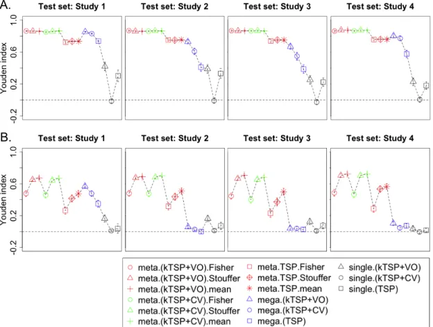
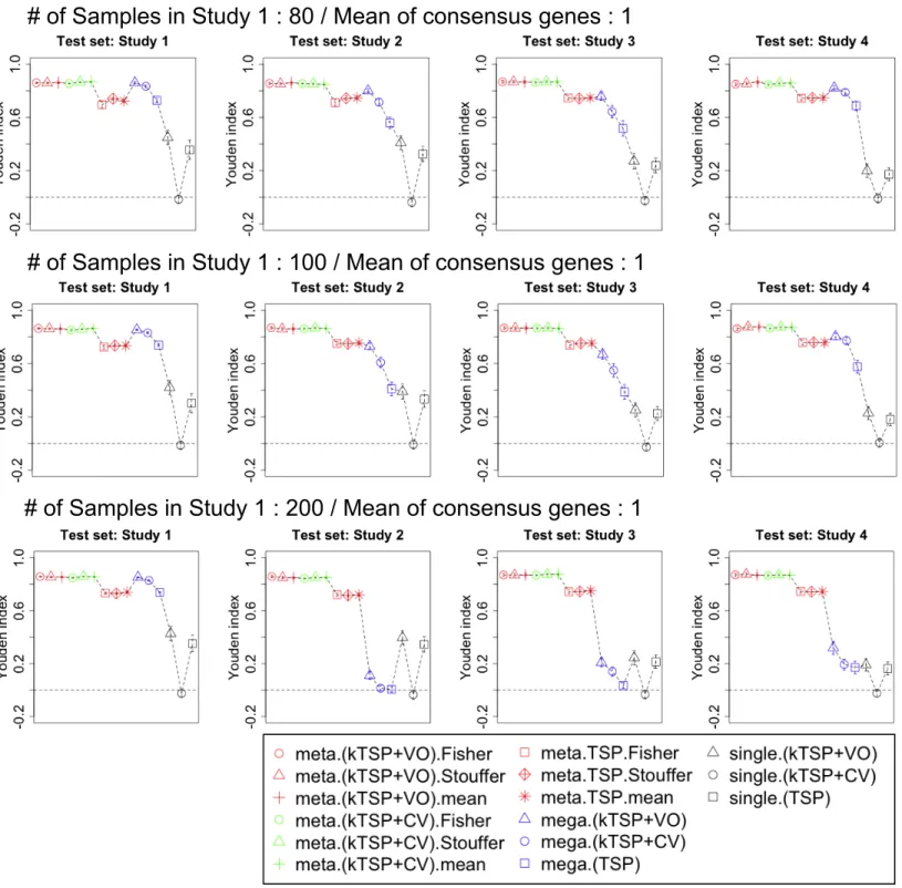
We repeated simulations for 50 times, and the results are benchmarked by averaged Youden index. Figure 5shows the simulation evaluation for di↵erent methods using Youden index. For meta-analysis methods, we tested three meta-analyzed approaches for selected TSPs (Fisher, Stou↵er, mean) and TSP/kTSP options. InkTSP, we have two further options (cross validation CV and variance optimization VO) to determine K, the number of TSPs for model construction. This gives a total of 9 meta-analysis methods to compare. In each meta-analysis evaluation, we take one study out as the test study, combine the remaining three studies to select the TSPs and construct the model, and finally use the model to predict samples in the test study. The result of Figure 2A in a stronger signal setting (µa = 1 or 1)

shows that all six meta-analysis methods by kTSP performed well (Youden Index = 0.851 -0.876). The three meta-analysis methods by TSP performed slightly worse (Youden Index = 0.723 - 0.759). In contrast, we also compared three mega-analysis and three single study analysis approaches. In mega-analysis approaches, the three training studies are normalized and combined into one study to construct the prediction model and evaluate in the test study. In single study analysis, the accuracy was evaluated by averaging inter-study accuracy from each of the three training studies to the test study. The result clearly shows inferior performance of the three mega-analysis approaches and poor performance of single study prediction. This confirms our hypothesis that prediction model from a single study may not be robust and accurate. Proper meta-analysis by combining multiple training studies improves the stability and accuracy of the model to predict an independent test study. Figure

9and 10shows results of di�