University of Wollongong
Research Online
Faculty of Business - Papers Faculty of Business
2014
The role of "other information" in analysts' forecasts
in understanding stock return volatility
Yaowen Shan
University of Technology Sydney Stephen Taylor
University of Technology Sydney Terry S. Walter
University of Sydney, [email protected]
Research Online is the open access institutional repository for the University of Wollongong. For further information contact the UOW Library: [email protected]
Publication Details
Shan, Y., Taylor, S. & Walter, T. (2014). The role of "other information" in analysts' forecasts in understanding stock return volatility. Review of Accounting Studies, 19 (4), 1346-1392.
The role of "other information" in analysts' forecasts in understanding stock
return volatility
Abstract
This study identifies "other information" in analysts' forecasts as a legitimate proxy for future cash flows and examines its incremental role in explaining stock return volatility. We suggest that "other information" contains information about fundamentals beyond that reflected in current financial statements and reflects firms' fundamentals on a more timely basis than dividends or earnings. Using standardized regressions, we find volatility increases when current "other information" is more uncertain and increases more in response to unfavorable news compared to favorable news. Variance decomposition analysis shows that the variance contribution of "other information" dominates that of expected-return news. The incremental role of "other information" is at least half of the effect of earnings in explaining future volatility. The results are more pronounced for firms with poor information environments. Overall, our results highlight the importance of including "other information" as an additional cash-flow proxy in future studies of stock prices and volatility. Disciplines
Business
Publication Details
Shan, Y., Taylor, S. & Walter, T. (2014). The role of "other information" in analysts' forecasts in understanding stock return volatility. Review of Accounting Studies, 19 (4), 1346-1392.
The role of “other information” in analysts’ forecasts in
understanding stock return volatility
Yaowen Shan
University of Technology, Sydney
Stephen Taylor*
University of Technology, Sydney
Terry Walter
University of Technology, Sydney and Sirca Limited
August 2013
Keywords: Other information, analysts’ forecasts, stock return volatility, variance
decomposition
JEL Classification: M41, G14, D84
We appreciate the suggestions of Stephen Penman (the editor), two anonymous reviewers, Mary Barth, Eli Bartov, Philip Brown, Robert Bushman, Jeff Callen, Dan Dhaliwal, Peter Easton, Neal Fargher, Jere Francis, Paul Griffin, Steve Huddart, John Lyon, Terry O’Keefe, Dan Simunic, Dan Segal, Tom Smith, Nasser Spear, Joseph Weber, Sarah Zechman, attendees at the AFAANZ Annual Conference, the University of Technology, Sydney Summer Research School, and the American Accounting Association Annual Meeting, as well as workshop participants at the Australian National University, University of Melbourne, University of New South Wales, University of Western Australia, and Victoria University, Wellington. The authors acknowledge research support from the Accounting and Audit Quality program of the Capital Markets Co-operative Research Centre, a research center established by the Federal Government of Australia.
*Corresponding author: School of Accounting
University of Technology, Sydney PO Box 123 Broadway
NSW 2007 Australia
ABSTRACT
This study identifies “other information” in analysts’ forecasts as a legitimate proxy for future cash flows and examines its incremental role in explaining stock return volatility. We suggest that “other information” contains information about fundamentals beyond that reflected in current financial statements and reflects firms’ fundamentals on a more timely basis than dividends or earnings. Using standardized regressions, we find volatility increases when current “other information” is more uncertain and increases more in response to unfavorable news compared to favorable news. Variance decomposition analysis shows that the variance contribution of “other information” dominates that of expected-return news. The incremental role of “other information” is at least half of the effect of earnings in explaining future volatility. The results are more pronounced for firms with poor information environments. Overall, our results highlight the importance of including “other information” as an additional cash-flow proxy in future studies of stock prices and volatility.
1 Introduction
Stock return volatility plays an essential role in understanding asset pricing, risk management, portfolio construction, derivative valuation, and the cost of capital.1 In theory, stock return volatility is a function of variation in cash flow news, expected return news, or both. Empirical research has endeavored to use fundamental variables such as dividends and accounting earnings to explain changes in volatility.2 However, both dividends and earnings have obvious limitations as cash flow proxies. Dividends tend to be smoothed and do not necessarily reflect future cash flows.3 On the other hand, accounting earnings reflect transaction-based revenue recognition and the accompanying matching of expenses, so they are unlikely to be a timely source of information about changes in fundamentals (Lev 1989). To the extent that accounting earnings are conservative (Watts 2003), there is also the difficulty of explicitly allowing for the differential timeliness with which earnings reflect good versus bad economic news. In fact, studies have argued that return volatility is too high to be justified by fundamental variables.4
We propose and empirically validate “other information” in analysts’ forecasts as a novel proxy for future cash flows. “Other information” refers to information contained in analysts’ earnings forecasts about a firm’s fundamentals beyond that reflected in current financial statements. After controlling for earnings, we confirm the incremental role of other information and find that it has significant and incremental explanatory power for future stock return volatility.
We use analysts’ consensus forecasts of next-year’s earnings to construct other information, consistent with our application of Ohlson’s (1995) linear information
1
Reasons why firm-level volatility is important include the following: the relation between perceived riskiness and cost of capital (Froot et al. 1992), the fact that high volatility can make stock-price-based compensation less effective and more costly (Baiman and Verrecchia 1995), the evidence that investment strategies based on volatility can earn significant abnormal returns (e.g., Ang et al. 2006), and, finally, the fact that arbitrageurs trading to exploit the mispricing of an individual stock face risks related to volatility in the sense that larger pricing error may be associated with higher volatility (Shleifer and Vishny 1997).
2
See, for example, Campbell (1991), Campbell and Vuolteenaho (2004), Irvine and Pontiff (2009), Sadka (2007), Vuolteenaho (2002), and Wei and Zhang (2006).
3 See Lintner (1956), Chen and Zhao (2009), and Chen et al. (2013).
4 Campbell (1991) and Campbell and Vuolteenaho (2004) find that dividend news explains only
15%-20% of the variation in market returns. In addition, several studies argue that volatility is likely to reflect market irrationality, trading on the part of retail (noise) traders, or both (Shiller 1981, Black 1986, Brandt et al. 2010, Foucault et al. 2011).
dynamics 5 It is well documented that analysts’ earnings forecasts capture forward-looking information about fundamentals from sources other than financial statements (see Cheng 2005a, Kothari 2001). However, we do not assume that the resulting other information variable represents all public and private information. Rather, we simply assume that earnings forecasts incorporate timely and unique information that is not readily available from financial statements. We also recognize that earnings forecasts may not incorporate all available information from financial statements, as prior studies suggest that analysts fail to fully account for the information contained in accounting earnings or earnings components.6 Accordingly, we view other information as an additional cash-flow proxy and consider the relative importance of accounting earnings and other information in influencing stock return volatility as an empirical question.
The theoretical link between other information and stock return volatility can be understood through an extension of the accounting version of the Campbell-Shiller model (Campbell and Shiller 1988a, Vuolteenaho 2002, Wei and Zhang 2006).7 We incorporate Ohlson’s linear information dynamics into the model and assume that the linear information dynamics error terms follow a conditional heteroskedastic process. We find that the conditional variance of other information is part of the conditional variance of stock returns. We therefore derive two testable predictions between other information and stock return volatility.8
Our first hypothesis is rather intuitive. Given the assumption of market efficiency, if
5 See Ohlson (2001) and Hand (2001). Ohlson (2001) suggests that “analysts’ consensus forecasts of
next-year earnings would seem to be a reasonable measure of expected earnings.” Dechow et al. (1999) use analysts’ earnings forecasts to measure the other information variables and report evidence that supports the economic modeling of residual income as an autoregressive process.
6
See Ramnath et al. (2008) for a review. Typically, the literature indicates that financial analysts do not fully adjust forecasts for earnings reversals, the earnings surprise in prior earnings announcements, and past abnormal accruals.
7
More generally, the theoretical link between other information and stock return volatility can be derived from discounted cash flow models and is not limited to the Campbell-Shiller (1988a) loglinear version. However, without loss of generality, the accounting version of the Campbell-Shiller (1988a) model enables us to derive a straightforward, closed form solution that is empirically testable. A related approach is used by Wei and Zhang (2006) and Irvine and Pontiff (2009), although with a different purpose.
8 Callen (2009) follows Ohlson (1995) and assumes that the error terms of Ohlson’s linear information
dynamics are mean-zero independent error terms with inter-temporally homoskedastic variance and suggests a link between the unconditional variance of stock returns and the unconditional variance of other information. However, this link is difficult to test empirically, because the unconditional variance of other information is assumed to be constant over time.
current other information is more uncertain, thereby increasing uncertainty about firms’ future cash flows, then future stock returns are expected to be more volatile. Our second hypothesis predicts that volatility increases more in response to unfavorable other information news than to favorable news. Other information news (i.e., the signed level of other information) can be thought of as an aggregate indicator of value-relevant events that have yet to have an impact on the financial statements. Previous studies provide consistent evidence that stock return volatility increases after the release of firm-specific news (Clayton et al. 2005) and also that volatility increases more in response to unfavorable news (Engle and Ng 1993, Rogers et al. 2009). This result can be understood in the context of either rational regime-switching models (Veronesi 1999) or behavioral finance theories (Barberis et al. 1998, Daniel et al. 1998).
We employ two widely used approaches to examine the incremental role of other information: standardized regression analysis and variance decomposition analysis. We recognize the advantages and limitations of both approaches and believe that the implementation of both methods provides robust conclusions and informative comparisons to the existing literature.9 We measure other information in two ways. The first approach follows Bryan and Tiras (2007), who measure other information as the residual from regressing one-year-ahead analysts’ forecasts of future earnings on current publicly available financial information (Ohlson and Shroff 1992, Manry et al. 2003). The second approach follows Dechow et al. (1999) and measures other information as analysts’ consensus forecasts minus earnings forecasts predicted from past financial accounting information.
A summary of our findings is as follows. Using standardized regressions, we find an economically significant relationship between other information and future volatility. Volatility increases when current other information is more uncertain and increases more in response to unfavorable other information news. A one standard deviation change in unfavorable other information news results in a more than 14% change in future volatility, significantly higher than the effect of favorable news (3%), while a one standard deviation increase in the uncertainty of other information is associated with a 17% increase in future volatility. The results are robust to controlling for other
volatility covariates and the existing cash-flow proxy (ROE and ROE volatility), technology bubbles, loss reporting, corporate governance attributes, financial reporting quality, and the inclusion of lagged stock return volatility.10 We find the effect of other information on volatility is slightly lower than that for earnings.
The results using a variance decomposition approach also confirm that other information is a legitimate cash-flow proxy and plays an incremental role in determining stock return volatility. Other information news explains around 70% of the total unexpected return variance, around eight times as large as the variance of expected-return news (9%). The variance of negative other information news is significantly higher than the variance of positive news. When comparing the relative importance of other information and earnings, we find that both dominate expected-return news and that the incremental variance of other information news is about half of the variance of earnings news in explaining stock return variations. As variance contribution is a function of persistence and variability, the lower variance contribution of other information relative to accounting earnings is due to the fact that other information is less persistent and has lower variability.
In addition, we find the relationship between other information and volatility holds for both systematic and idiosyncratic volatility.11 This result suggests that other information has substantial undiversified variation and contains both firm-specific and market-level information. This is consistent with recent studies examining the predictive content of aggregate earnings (Ball et al. 2009), earnings announcements (Cready and Gurun 2010), accrual and cash flow components of earnings (Hirshleifer et al. 2009), and earnings dispersion (Jorgensen et al. 2012).
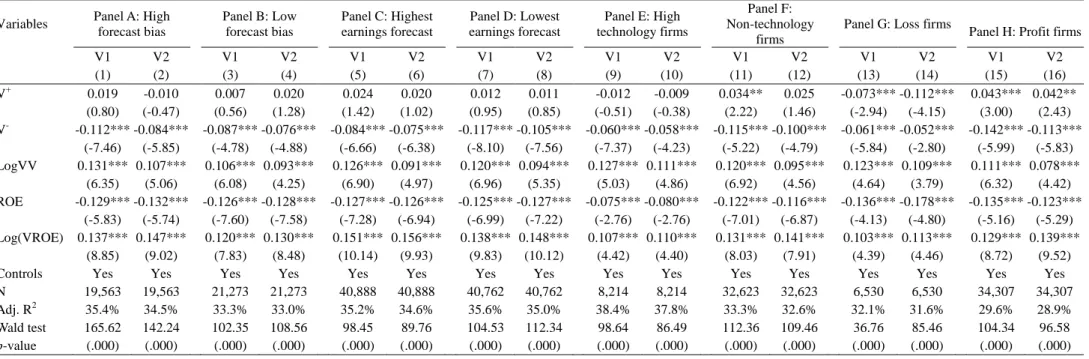
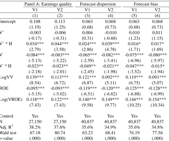
Finally, we document that the relationship between other information and future volatility is more pronounced for firms with a relatively poor information environment. We use earnings quality, forecast dispersion, and forecast bias as proxies for differences
10 See Chan et al. (2001) and Schwert (2002) for technology bubbles, Givoly and Hayn (2000) for loss
reporting, Ferreira and Laux (2007) for corporate governance effects, and Rajgopal and Venkatachalam (2011) for financial reporting quality. Our results are also robust to several different measures of stock return volatility, different sample periods, different industry categories, and different econometric estimations such as Fama-MacBeth (1973) regressions and fixed effect regressions. See section 4.3 for additional discussion.
11
Total volatility is decomposed into systematic and idiosyncratic components by using the CAPM and the Fama-French three factor model (Fama and French 1993, 1996), respectively.
in firms’ information environments. Our results imply that financial analysts place greater weight on other information, and lower weight on reported accounting information, when following firms with a poor information environment. This is also consistent with Bryan and Tiras (2007), who suggest that Ohlson’s (1995) valuation model better describes market pricing in poor information environments.
Our study makes several contributions. First, we are among the first to propose and validate other information as a novel and legitimate proxy for future cash flows. We show that the incremental role of other information is at least half of the role of accounting earnings in explaining both market-wide and firm-specific volatility. Although Chen et al. (2013) use analysts’ forecast revisions for cash flow estimation, our approach differs from Chen et al.’s (2013) in important ways. Because we use earnings forecasts rather than forecast revisions to compute cash-flow news, our approach can be directly applied to the variance decomposition framework and compared with prior studies. Chen et al., however, require a different definition of news that is not directly comparable to the results obtained from other methods. Further, our approach is relatively easy to implement. In contrast, Chen et al. require computation of the implied cost of capital from analysts’ forecasts and then define cash-flow news as the price change calculated from a pricing function by assuming constant implied cost of capital. Our approach may also generate more reliable cash-flow news estimates, as their approach likely amplifies the measurement error in cash-flow proxies attributable to the intermediate step of implied cost of capital estimation.
Second, by introducing other information, we extend the variance decomposition methodology of Campbell (1991), Vuolteenaho (2002), and Callen and Segal (2004) to evaluate and compare the variance contribution of accounting earnings and other information. We also contribute to broader capital market research by addressing the question of what drives stock return volatility cross-sectionally. While a limited amount of evidence relates volatility with financial disclosure (Bushee and Noe 2000), firm age (Pástor and Veronesi 2003), accounting earnings (Wei and Zhang 2006), governance mechanisms (Ferreira and Laux 2007), and financial reporting quality (Rajgopal and Venkatachalam 2011), we identify other information as an additional fundamental determinant of volatility. Taken together, our results highlight the importance of other information and suggest that future studies that attempt to explain stock prices or
volatility should consider other information as a cash-flow proxy.
Our paper also adds to the literature on accounting-based valuation models. Our results indicate that unfavorable other information is more important in explaining volatility and that the relationship between other information and volatility is more apparent for firms with a poor information environment. While several studies find that Ohlson’s model is of limited empirical validity (Bar-Yosef et al. 1996, Myers 1999), our evidence on volatility indicates that Ohlson’s valuation model is more descriptive for firms with unfavorable other information and poor information environments.
Finally, our results have important implications for corporate disclosure policy. The disclosure of other information is often discretionary and released strategically. Our evidence of a positive relationship between the uncertainty of other information and future volatility suggests that improved disclosure of other information helps to reduce uncertainty about firms’ fundamentals and thus firm-specific risk.12 However, more frequent disclosure of value relevant information may not be advantageous for firms with poor information environments, as both good and bad other information is associated with increased volatility. Evidence of an asymmetric effect of other information news on future volatility also supports the view that managers have incentives to delay disclosure of bad news relative to good news (Kothari et al. 2009), as the release of bad news tends to increase a firm’s expected risk much more than the release of good news.
The rest of the paper is organized as follows. Section 2 develops our model incorporating other information and hypotheses. Section 3 discusses sample construction, the measurement of other information variables, and descriptive statistics. Section 4 and Section 5 present the results of standardized regressions and the variance decomposition approach respectively. Section 6 examines how firms’ information environment affects the relationship between other information and volatility. Section 7 concludes.
12 For example, an increase in the frequency and precision of disclosure might increase the number of
observations drawn from the firm’s underlying earnings series and thus lower investors’ uncertainty about the parameters of the distribution of future earnings.
2 Motivation
2.1 The model
At the fundamental level, stock prices are the sum of expected future payoffs adjusted by the appropriate discount rate. Campbell and Shiller (1988a, 1988b) use a loglinear approximation to represent the relationship between prices, dividends, and returns. Using a variance decomposition approach, Campbell (1991), Campbell and Ammer (1993), and Campbell and Vuolteenaho (2004) find that expected-return news dominates dividend news in driving equity returns at the market level. However, although the literature often focuses on dividends as a proxy for future cash flows, dividends are subject to the discretion of managers and do not necessarily reflect changes in fundamentals.
To mitigate this problem, Vuolteenaho (2002) extends the Campbell-Shiller model using the accounting clean surplus relationship (Ohlson 1995), replacing dividends with accounting earnings. The result is a new link between unexpected stock returns and changes in future discount rates and expected future ROEs as follows:
it 0 j j i,t j t j t 0 j j i,t j t it t-it-E r ΔE (ROE f E r r
) 1 (1)where rit is the return on stock i in period (t-1, t); ROEi,t+j is the return on equity in
period (t+j-1, t+j); ft+jis the risk-free rate for period (t+j-1, t+j); ρ is a constant slightly
less than one; and κit is an approximation error. In equation (1), Et-1 is the expectation conditional on the information available at t-1, and ∆Et=Et - Et-1 is the change in expectation from t-1 to t.
The variance of unexpected stock returns can be decomposed into three components as follows, ) , cov( 2 ) ) ( ) (rit Et 1rit Var Nr.i,t Var(Ncf,i,t Nr.i,t Ncf,i,t Var (2)
where Ncf,i,t (cash-flow news) represents
0 j j t j t i, j t (ROE f E ) , and Nr,i,t
(expected-return new) represents
0 j t j t i, j t r
E . Vuolteenaho (2002) finds the cash-flow news is dominant in the right hand side of equation (2) at the firm level, and the variance of cash-flow news is more than twice that of expected-return news.
Following Wei and Zhang (2006), we take a first approximation of the unexpected-return variance and focus our attention on the conditional variance of the cash flow news. The relationship can be derived from equation (2) as:
1 , 1 1
it 0 j j t i, j t t it t (r ) Var E ROE Var (3)where i,t-1encompasses the conditional variances of the expected-return news and the conditional covariance between the cash flow news and expected-return news.
The key fundamental variable in our study is other information. Other information is expected to be a timelier source of information about changes in fundamentals, compared to either dividends or accounting earnings, the latter having been argued to be a backward-looking measure (Ball and Shivakumar 2008). Following Vuolteenaho (2002), we use an equivalent to Ohlson’s ROE-based linear information dynamics based on abnormal earnings. The economic intuition behind Ohlson’s linear information dynamics is that competition will erode above-normal returns, while firms experiencing below-normal rates of return will either recover or eventually exit. Providing that the normal level of ROE is equal to r, a typical firm’s ROE satisfies the following autoregressive process with conditional heteroskedastic error terms:
t t t t r w ROE r v u ROE ( 1 ) 1 , (4a) ) , ,..., , ( ) ( 1 2 2 2 2 1 1 t t t t k t t u g u u u u Var , (4b) t t t v v 1 , (4c) ) , ,..., , ( ) ( 1 2 2 2 2 1 1 t t t t k t t f Var , (4d) where vtis other information, namely information about future earnings not in current
earnings; w and φ are fixed persistence parameters that are nonnegative and less than one; and utand εt are error terms independent of each other and are assumed to follow a
conditional heteroskedastic process (Wei and Zhang 2006).13
13 We follow Callen (2009) and assume that u
tand εt are independent of each other to simplify the exposition. Relaxing this independence assumption would result in an additional covariance term in equation (6) and equation (7). However, the focus of our study is on the (incremental) role of other information in explaining future volatility. Furthermore, the assumption that the error terms follow a conditional heteroskedastic process ensures that the predicted link between the conditional variance of stock returns and the conditional variance of other information is empirically testable. In other words, based on this assumption, the predicted link suggests that the conditional variance of stock returns is a function of time-varying other information.
After some simple algebra, we have t t t t c wROE v u ROE 1 1 , (5a) ) , ,..., , ( ) ( 1 2 2 2 2 1 1 t t t t k t t u g u u u u Var , (5b) t t t v v 1 , (5c) ) , ,..., , ( ) ( 21 22 2 1 1 t t t t k t t f Var , (5d) where c (= r(1 - w)) is the intercept.14
If ROEs follow process (5), it is easy to derive the following (see Appendix A for details): ) ) ) ) ( 2 2 t 1 -t 2 t 1 -t 2 0 j j t j t 1 t Var ( w (1 ) (1 u ( Var ) w (1 1 ROE E Var
(6) and thus 1 t t k t t t 2 t k t t t 2 t 1 t f w (1 ) (1 u u u u g ) w (1 1 r Var ( , ,..., , ) ) ( , ,..., , ) ) ( 2 21 22 2 1 2 1 2 2 2 2 1 (7) The above model suggests that the conditional variance of other information contained in analysts’ forecasts (Vart-1(εt)) is part of the conditional variance of stock returns. Inthe empirical analysis below, we adopt a nonparametric approach in constructing proxies for the conditional variance of other information without modeling the stochastic process for other information. In particular, following Wei and Zhang (2006), we use two variables available at time t-1, realized volatility of other information (ε2t-1) and realized other information itself (εt-1), as inputs to the nonparametric estimators. The use of these two nonparametric estimators to construct the conditional variance of other information is also supported by prior studies. For example, Adut et al. (2009) provide evidence that the variance of analysts’ earnings forecasts is smaller when the expected or actual news about earnings is relatively better.
2.2 Variance decomposition method
The relationship between other information and stock return volatility can also be described in a variance decomposition framework. As discussed above, the unexpected stock return is determined by cash flow news and expected-return new as:
14 The ROE-based information dynamic can also be directly derived from Ohlson’s (1995) linear
information dynamics using the assumption that the growth rate of book value is constant over time. Easton (1998) and Callen (2009) also utilize similar information dynamics.
t i r t i cf it t-it-E r N N r 1 ,, ,, (8)
Accordingly, the variance of unexpected stock returns can be decomposed into the variance of cash-flow news, the variance of expected-return news and the covariance as in equation (2). If we use other information, v, as the key proxy for future cash flow, we will replace Ncf in equation (2) by other information news, Nv:
) , cov( 2 ) ) ( ) (rit Et 1rit Var Nr.i,t Var(Nv,i,t Nr.i,t Nv,i,t Var (9)
As both accounting earnings and other information can be considered as future cash-flow proxies, it is unclear which of these contributes more to changes in stock return volatility. To examine the relative importance of earnings news and other information news, we follow the spirit of Ohlson’s linear information dynamics and assume that the inclusion of other information provides a better measure of future cash flows. In such respect, the unexpected stock return is now determined by three components: accounting earnings news (Nroe), other information news (Nv), and
expected-return news (Nr) as below:
t i r t i v t i roe it t-it -E r N N N r 1 ,, ,, ,, (10)
Taking the variances of both sides of equation (10) yields:
) , cov( 2 ) , cov( 2 ) , cov( 2 ) ) ) ( ) ( , . , . , . , . 1 t i, v, t i roe t i, v, t i r t i, roe, t i r t i, r, t i, v, t i roe it t it N N N N N N N Var( N Var( N Var r E r Var (11)
Equation (9) and (11) are used to motivate our variance decomposition analysis. Equation (9) assesses the relative importance of other information news and expected-return news in explaining stock returns. Equation (11) further assesses the relative importance of other information news, accounting earnings news, and expected-return news. The greater the variance of any factor on the right side, the more power that factor has in explaining unexpected stock returns. The relative variance contribution is therefore defined as the contribution of each factor to the variance of stock returns.
To implement the return variance decomposition, we follow Vuolteenaho (2002) to estimate the one-period expected return, cash flow news, and discount rate news series
using a loglinear vector autoregressive (VAR) model as below:
Zt = AZt-1 + ηt (12)
where Zt is a vector of (mean-adjusted) log stock returns, log other information
variables, log accounting earnings, and log book-to-market ratio at time t. A is the VAR coefficient matrix. The error terms, ηt, are vectors of shocks and assumed to have a
variance-covariance matrix Ω and be independent of everything known at t-1.
With the VAR model expressed in this form, the three unexpected stock return components, accounting earnings news (NROE), other information news (Nv), and
expected-return news (Nr), can be calculated as:
Nr,t = e1’ ρA (I - ρA)-1 ηt = λ1ηt Nv,t = e2’(I - ρA)-1 ηt = λ2ηt Nroe,t = (e1’ - e2’)(I - ρA)-1 ηt = λ3ηt
where ’ denotes the transpose operator, ek’ = [0, …, 1,…, 0] is a vector with one as the kth element and zero otherwise.
The variance and covariance of the variance decomposition as expressed in equation (11) can be computed as:
var(Nr,t) = λ1’Ω λ1 var(Nv,t) = λ2’Ω λ2 var(Nroe,t) = λ3’Ω λ3 cov(Nr,t, Nv,t) = λ1’Ω λ2 cov(Nr,t, Nroe,t) = λ1’Ω λ3 cov(Nv,t, Nroe,t) = λ2’Ω λ3 2.3 Hypothesis development
Equation (7) suggests a positive relationship between realized volatility of other information (ε2t-1) and future stock return volatility. The intuition is as follows. Given the assumption that stock prices fully reflect the implications of current earnings for future earnings, increased uncertainty in current other information is expected to reflect increased uncertainty about future cash flows, and so on average future stock returns will be more volatile.15 Hence the uncertainty of other information reflected in analysts’
15
A large part of the accounting literature suggests that the market is naive in recognizing the time-series properties of earnings, resulting in significant post-earnings-announcement abnormal
forecasts will be associated with fluctuations in future stock returns. Therefore our first hypothesis is stated as follows:
H1: The future volatility of a firm’s stock returns increases if current other information is more uncertain.
The relationship between realized other information (εt-1) and future stock return volatility is also of particular interest, as realized other information can be thought of as the aggregate news of all value-relevant events that have yet to have an impact on the financial statements. Volatility can be linked to the quantity and quality of information pertaining to firm’s fundamentals. According to this view, the most important process affecting volatility is the news arrival process (Andersen 1996). Numerous studies have examined price reactions to news releases, typically concluding that firm-specific news increases stock return volatility after the release of information (Clayton et al. 2005). Since volatility tends to be clustered (Schwert 1989), the effect of news releases tends to continue for some time. This implies that stock return volatility is smallest when there is no news (i.e., the level of other information is equal to zero).16
On the other hand, extensive research has found that stock return volatility increases more in response to bad news than in response to good news (i.e., volatility asymmetry). The ARCH-related literature provides a rich set of studies on this issue (Engle and Ng 1993). Beyond research using a time-series setting, previous cross-sectional studies, such as Rogers et al. (2009), also find that the effect of management earnings forecasts on short-term volatility is mainly attributable to forecasts that convey bad news.
Two strands of literature attempt to provide a theoretical framework to better explain the asymmetrical response of stock return volatility to news. The first, based on research in behavioral psychology, suggests that investors inappropriately extrapolate past performance. Therefore bad news has a particularly telling impact after a long
returns (Kothari 2001). However, recent studies refine our understanding of the drift. For example, Brown and Han (2000) suggest the market is not entirely naive but rather underestimates the parameters of the true process.
16 Damodaran (1985) suggests that investors react to news in different ways depending on how they
think the information affects the future payoff of their assets and how big a surprise the information was for them. Given that the level of other information is an aggregate indicator of all other information news, the relation between other information news and volatility is ambiguous.
period of good news because it has the effect of correcting overoptimistic projections (Barberis et al. 1998, Daniel et al. 1998).17 The second strand of literature relates to regime-switching rational equilibrium models. Veronesi (1999) suggests that the asymmetric response occurs because news affects not only expected cash flows but also the risk associated with the probability of a regime shift.18
Overall, we expect that the response of future stock return volatility to unfavorable other information news to be stronger than for favorable news. Our second hypothesis is stated as follows:
H2: Future stock return volatility increases more in response to unfavorable other information than for favorable other information.
We also separately consider whether other information contained in analysts’ forecasts (mainly) drives cross-sectional differences in systematic or idiosyncratic volatility. It would not be surprising for hypotheses one and two to hold for idiosyncratic volatility, because the finance literature shows that idiosyncratic volatility accounts for most of total stock return volatility (Campbell et al. 2001, Wei and Zhang 2006). While our theoretical model does not offer any guidance on systematic volatility or discount rate news, we expect similar results for systematic volatility. Ball et al. (2009) find that accounting earnings have substantial systematic components and undiversified variation and that systematic earnings risk is correlated with market-wide return risk. The above notion has been supported by follow-up research on market reaction to earnings announcements (Cready and Gurun 2010), accrual and cash flow components of accounting earnings (Hirshleifer et al. 2009), and earnings dispersion (Jorgensen et al. 2012). Similar to accounting earnings as a proxy for future cash flow, other
17 For example, to reconcile the empirical findings of overreaction and underreaction, Daniel et al.
(1998) use psychological concepts of overconfidence and self-attribution to construct a model of investor sentiment in the sense that “stock prices overreact to private information signals and underreact to public signals” (p. 1,841). Barberis et al. (1998) model investors as typically (but not always) believing that earnings are more stable than they really are. In such a situation, bad news following a series of good news events generates a large negative response because it is a surprise, whereas good news generates little response because it is anticipated.
18 Veronesi (1999) suggests that, in good times, bad news decreases future expected cash flow and
increases investors’ uncertainty about a regime shift in the underlying cash flow process. Risk-averse investors thus require a higher discount rate for bearing the increasing risk of a regime shift, and this reinforces the effect of the bad news in good times. However, as there is no similar reinforcement in the case of good news, volatility increases more in response to bad news.
information would be expected to be associated with systematic volatility if it has significant undiversified variation and contains both firm-specific and market-level information. Our third hypothesis is therefore stated as follows:
H3: Both future systematic volatility and idiosyncratic volatility of a firm’s stock returns will increase if current other information is more uncertain or more unfavorable.
2.4 Standardized regression vs. variance decomposition approach
We use two distinct empirical approaches to examine the incremental role of other information in determining stock return volatility: standardized regression analysis and variance decomposition analysis. Each method has advantages and limitations. However, employing both enables us to draw relatively robust conclusions and provide informative comparisons with prior literature.
First, we use regression analysis consistent with many prior volatility studies.19 The use of regression analysis is consistent with the theoretical predictions and hypotheses derived from equation (7). It also enables us to control for a large set of volatility covariates to mitigate spurious correlations. However, statistical inferences and interpretation based on the magnitude of regression coefficients are difficult, because the magnitude of an ordinary regression coefficient depends on the scale of both the dependent variable and the independent variables. To identify and interpret the economic significance of other information variables in determining volatility, we use standardized regressions (Bennett et al. 2003, Ferreira and Matos 2008). In particular, we standardize both the independent and dependent variables, such that all variables have the same mean (zero) and standard deviation (one), so that all estimated coefficients based on standardized regressions are presented in comparable units. The interpretation of such standardized regression coefficients is the expected standard deviation change in the dependent variable given a one standard deviation change in the independent variable.
We also adopt a variance decomposition approach in line with volatility studies such as
19
See, for example, Pástor and Veronesi (2003), Wei and Zhang (2006), Ferreira and Laux (2007), Irvine and Pontiff (2009), Brandt et al. (2010), and Rajgopal and Venkatchalam (2011).
Campbell and Shiller (1988a, 1988b), Vuolteenaho (2002), and Callen and Segal (2004). The variance decomposition analysis provides a variance-based approach to measure value relevance of other information. It offers an intuitive representation of the (relative) importance of other information, accounting earnings, and expected-return news. Moreover, it explicitly controls for changes in expected returns over time. This is important for assessing the value relevance of other information, because small changes in expected discount rates can have a large impact on stock returns, especially when expected returns are persistent (Campbell et al. 1997).
However, variance decomposition requires a system of VAR equations, which cannot include a large set of volatility covariates simultaneously due to estimation complexity. More importantly, several studies have identified empirical limitations associated with this approach (Ball et al. 2009, Chen and Zhao 2009). For example, the expected-return news in the variance decomposition approach cannot be accurately measured due to low predictive power, and the cash flow news, when treated as the residual, inherits the large misspecification error of the expected-return news. A missing state variable in the variance decomposition approach is likely to alter the empirical conclusion. In contrast, such model misspecification is much less damaging for regression analysis. Even if a factor is missing in a regression model, we can still draw statistical inferences about the specified factors despite increased noise, if the omitted variable is not highly correlated with the specified factors.
3 Data, variable measurement and descriptive statistics
3.1 Sample
The empirical analysis employs annual accounting data, daily stock return data, and analysts’ forecasts data from the merged Compustat XPF, I/B/E/S, and CRSP database for the period of 1981-2011. Following prior literature, for a firm-year to be included in the sample, it must satisfy the following requirements: (1) nonmissing and positive book value of equity at time t-1 and t-2, where t denotes time in years; (2) nonmissing one lag of net income; and (3) a valid figure for market value of equity available for t-1 and t-2. In addition, we exclude firms with t-1 market equity less than $10 million and a book-to-market ratio more than 100 or less than 0.01 to screen out possible data errors
and mismatches.20 To mitigate the undue influence of outliers, we winsorize the top and bottom one percentile of key variables used in the regression analysis.21 Consensus analyst forecast data are extracted from the I/B/E/S unadjusted summary file. To ensure that forecasts are current and released after the firm has filed its annual report with the SEC and hence that earnings, book values, and other accounting information are publicly available, one-year ahead earnings forecasts are extracted as of the fifth month after the fiscal year-end.22 We require that there be at least three earnings forecasts available. The interaction of CRSP, Compustat, and I/B/E/S databases produces a final sample of 42,700 firm-year observations after applying all the above requirements. Appendix B summarizes the measurement of all variables.
Consistent with Vuolteenaho (2002), the annual stock returns (RETURN) are compounded from CRSP monthly returns, recorded from the beginning of the sixth month after the fiscal year-end.23 We require a valid stock return during the last month of the fiscal year to ensure that the return predictability is not spuriously induced by stale prices. If the firm was delisted we use the delisted return when available in CRSP. If the delisting return is missing, we investigate the reason. If the delisting is performance based, we assume a -30% delisting return. Otherwise, we assume a zero delisting return.
Stock return volatility is computed as the sample variance of daily stock returns (in percentage) over the same recording period as stock returns.24 The systematic and idiosyncratic volatilities are computed as follows. First, a factor model is used to decompose the daily stock returns into systematic and idiosyncratic return components. The factor model used is either the CAPM or the Fama-French three-factor model. Daily individual stock returns are applied to the models to obtain the daily systematic and idiosyncratic return components.
20 The results remain similar if we do not impose any requirement for market equity.
21 Our results remain quantitatively similar if we trim the top and bottom percentiles of key variables
or keep them in the analysis.
22 The Compustat data reveal that more than 95% firms release their annual reports within three
months after the financial year. Our results are similar if we use earnings forecasts from I/B/E/S in the fourth month after the fiscal year.
23 The results are quantitatively similar if we calculate returns from the fourth or fifth month after the
fiscal year-end.
In analyzing the relationship between the uncertainty of other information and stock return volatility, we use several control variables that have been previously identified, including return on equity (ROE), the variance of return on equity (VROE), firm size (SIZE), firm age since listing (AGE), financial leverage (LEV), book-to-market ratio (BM), contemporaneous stock return (RETURN), analyst forecast bias (BIAS), and forecast dispersion (DISP).
ROE is measured as net income (NI) divided by lagged book value of equity (CEQ). When the value of ROE is less than -100%, it is treated as a missing value because the log transformations for the VAR model are not possible for any variable less than 0. VROE is the sample variance of yearly ROE observations over the past five years for a minimum of three observations. Age is measured as the logarithm of the number of months from the firm’s IPO date. If IPO dates are unavailable, we use the first tracking date of the firm appearing in the CRSP. SIZE is the logarithm of the firm’s market value of equity, where market value of equity is defined as common shares outstanding (CSHO)multiplied by the stock price (PRCC_F). LEV is equal to the sum of total long-term debt (DLTT) and debt in current liabilities (DLC), divided by total assets (AT). Book-to-market ratio (BM) is book value of equity (CEQ) divided by the market value of equity. In line with prior literature, firms with lower ROE and higher VROE are expected to experience higher stock return fluctuations (Pástor and Veronesi 2003, Wei and Zhang 2006). We expect that younger and smaller firms will experience higher stock return volatility and a negative relationship between BM and volatility because firms with greater growth opportunities are more likely to experience greater fluctuation in stock returns (Bushee and Noe 2000, Ferreira and Laux 2007).
We also control for attributes of analysts’ forecasts to ensure that any link between the uncertainty of other information and stock return volatility is not driven by specific properties of analysts’ forecasts, such as forecast dispersion and forecast bias. Studies by Ajinkya and Gift (1985) and Daley et al. (1988) find that the ex ante variability of stock returns around earnings announcements is positively related to analysts’ forecast dispersion. Ackert and Athanassakos (1997) further show that analysts’ forecast dispersion is positively associated with analyst optimism. We measure forecast bias (BIAS) as the absolute difference between the one-year-ahead consensus mean analyst forecast of year t+1 earnings per share reported in the fifth month after the fiscal
year-end and the actual earnings per share reported in I/B/E/S, divided by stock price at the fiscal year-end. Forecast dispersion (DISP) is defined as the standard deviation of one-year-ahead consensus analyst forecasts of year t+1 earnings per share, standardized by the absolute value of consensus forecasted earnings per share.25
3.2 Measurement of other information
Our other information variable is measured using two distinct approaches. We use V1 (V2) to represent the other information variable estimated from the first (second) approach outlined below. As discussed in section 2, we use realized volatility of other information as a nonparametric estimator of the conditional variance of other information, denoted as VV1 (VV2). VV1 (VV2) is defined as the sample variance of the yearly V1 (V2) observations over the past five years (with a minimum of three observations).
Following earlier studies, our first measure of other information is the residual from regressing one-year-ahead analysts’ forecasts on current publicly available financial information (Bryan and Tiras 2007, Ohlson and Shroff 1992, Manry et al. 2003).26 We estimate the following cross-sectional regression to identify other information contained in analysts’ forecasts that is not contained in current earnings or book value:
t i t i t i t i, c0 c1BVPS, c2ROE, v, FROE (13) where, for each firm i, FROEi,t is the one-year-ahead consensus mean analyst forecast
of earnings per share at year t divided by book value of equity per share at year t; BVPSi,t is net book value of equity per share at year t; and vt is a residual that proxies for
other information.27 As the actual EPS reported in I/B/E/S is more consistent with the analysts’ EPS forecasts, we also estimate an alternative version of equation (13) where ROEi,t is replaced by AROEi,t (namely I/B/E/S ROE, measured by the actual earnings
per share of year t+1 reported in I/B/E/S, divided by book value of equity per share at year t). Equation (13) is estimated separately for each fiscal year, with each regression using all available observations from that year.28
25
The deflator is commonly used to reduce heteroskedasticity. We also standardize by the firm’s stock price at the end of year. The main results are qualitatively similar.
26 Our results remain similar if we follow Manry et al. (2003) and exclude BVPS as a regressor in
equation (9).
27 The results are similar if we use the consensus median forecasts rather than the mean forecast of
earnings per share.
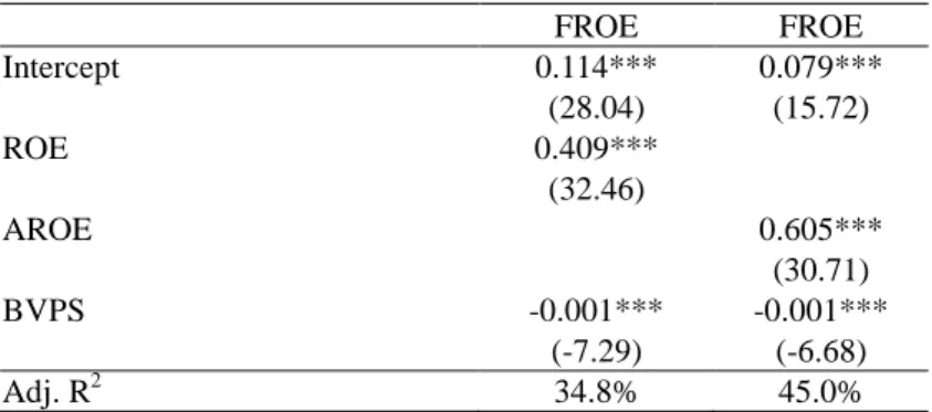
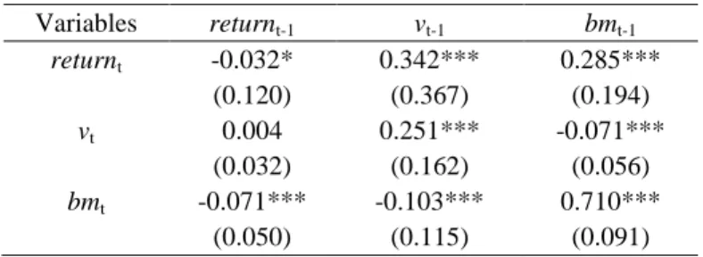
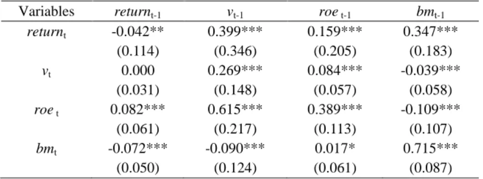
Panel A of Table 1 reports results for the cross-sectional estimation of equation (13) for the pooled sample from 1981 through 2010. The explanatory power of the regression using ROE (AROE) is 34.8% (45.0%). The intercepts of both regressions are positive and significant, consistent with a systematic positive difference between the one-year-ahead forecasts and past actual earnings (i.e., optimistic forecasts).
Our second approach reflects Ohlson’s (2001) suggestion that the other information variable, vt, can be interpreted as the difference between the conditional expectation of
earnings for period t+1 based on all available information and the expectation of earnings based only on current period earnings.29 We follow Dechow et al. (1999) and Ohlson (2001) and use consensus analyst earnings forecasts to measure the year t conditional expectation of year t+1 earnings. The expectation of earnings based only on current period earnings is estimated from the AR(1) process of ROE. Thus the other information variable can be interpreted as vt = FROEt – (c + wROEt). Here
FROEt is the one-year-ahead consensus analyst forecast of earnings per share at year t+1, divided by book value of equity per share at year t. Both c and w are parameters of the ROE process.
We follow Fama and French (2000) and Cheng (2005b) and use conditional cross-sectional estimation of w to capture cross-sectional variation in the earnings persistence as a function of its economic determinants. Economic determinants employed include market share (the ratio of firm’s sales to total industry sales), firm size (the natural logarithm of total assets), R&D intensity (R&D expenditures over sales), advertising intensity (advertising expenditure over sales), capital intensity (the ratio of depreciation, depletion, and amortization to sales), the magnitude of earnings (the absolute value of ROE), the magnitude of special items (the absolute value of the ratio of special items to lagged book value), and the magnitude of total accruals (the absolute value of the ratio of total accruals to lagged total assets). The measurement of the determinants of ROE persistence is summarized in Panel D of Appendix B.
observations in the sample from previous years, going back as far as 1981. The main results hold.
29 Ohlson (1995) defines his other information variable, v
t, as the difference between the conditional expectation of abnormal earnings for period t+1 based on all available information and the expectation of abnormal earnings based only on current period abnormal earnings.
The conditional value of ROE persistence (w) used in calculating the other information variable is estimated as follows. We first estimate earnings autoregressive regressions in which each of the eight determinants of ROE persistence are included as interactive effects: 1 , , , , 1 , ( )
it it n 1 k t k k t i 0 t i c bROE b F ROE u ROE (14)where Fk,t is the k'th persistence determinant, k=1, 2, …,n; n is the number of variables
used in the estimation with a maximum of eight. Equation (14) is estimated separately for each fiscal year, with each regression using all available observations from that year.30 The conditional estimated value of ROE persistence for each firm-year is then computed using the parameter estimates from this regression:
8 1 k t k t k t 0, t i b b F wˆ, ˆ ˆ, , (15)If one of the variables required to calculate w is missing, then the respective term is set equal to 0.31
The results reported in Panel B of Table 1 are the time-series average of the cross-sectional estimates for the annual regressions. All of the eight determinants are found be statistically significant and consistent with their hypothesized signs. Consistent with Dechow et al. (1999) and Cheng (2005b), the coefficients associated with ROE magnitude, special items, and total accruals are all significantly negative, indicating that earnings persistence is lower when earnings contain more transitory accounting items. Market share, firm size, and proxies for firm-level barriers to entry (R&D and advertising intensity) all have positive coefficients.
[Insert Table 1 here]
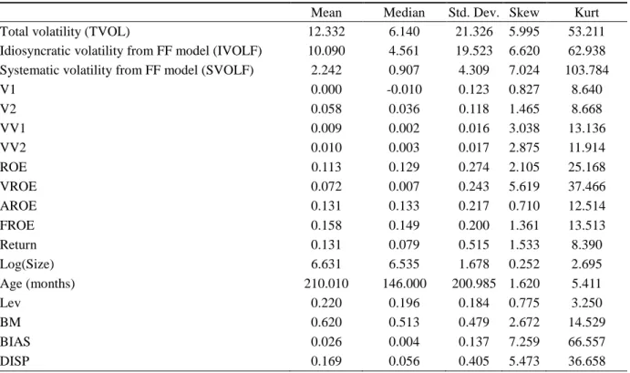
3.3 Descriptive statistics
Table 2 reports descriptive statistics for the variables used in the analysis. The average firm has a market capitalization of $758 million, a book-to-market ratio of about 0.62, a
30 Following Dechow et al. (1999), we also estimate a separate regression for each fiscal year, with
each regression using all available observations from previous years, going back as far as 1950. The results are similar to those reported in the text.
31
A sample restricted to observations without missing values for each persistence determinant yields qualitatively similar results.
tracking period in Compustat of 17.5 years, and financial leverage of 22% of total assets. For brevity, in the following we concentrate on the other information variables estimated from ROE, but all results continue to hold when using estimates from AROE. Results indicate that average (median) annual total volatility is 12.33% (6.14%). Outliers and nonnormality result in a substantial difference between the mean and median, as evidenced by skewness and kurtosis values of 6.00 and 53.21 respectively. Patterns of positive skewness and significant leptokurtosis are also found in other measures of stock return volatility, the volatility of other information, and ROE volatility. Therefore, following Durnev et al. (2004), we apply a logarithmic transformation. The values of skewness and kurtosis of the natural logarithm of total volatility are equal to 0.34 and 3.12 respectively, indicating the natural logarithm of these variables is more symmetric and normal. Decomposition of total volatility shows that the total variation of stock returns mainly reflects idiosyncratic volatility, which is about 82% of total volatility.
The mean of V1 is 0 by construction, compared to that of V2 (0.058). Recall that the other information variable is assumed to have a mean of zero and a normal distribution. This suggests that the second measure of other information (V2) may incorporate the influence of forecast bias.32 The standard deviations of V1 and V2 are 0.123 and 0.118 respectively, both of which are lower than the standard deviation of ROE (0.274). The mean of VV1 is 0.009, slightly lower than that of VV2 (0.010).
[Insert Table 2 here]
4 Results using standardized regression
4.1 Other information and total volatility
We begin with a set of standardized regressions of total volatility on other information variables as well as the control variables discussed above:
t i t i 12 t i 11 t i 10 t i 9 t i 8 t i 7 t i 6 t i 5 t i 4 t i 3 t i 2 t i 1 0 t i DISP BIAS Log(BM Lev Age Size R Log(VROE ROE Log(VV V V Log(VOL , 1 , 1 , 1 , 1 , 1 , 1 , , 1 , 1 , 1 , 1 , 1 , , ) ) ) ) (16) where VOLi,t is the volatility measure of stock i in year t, as defined in (8). Vi,t-1 is the measure of other information in year t-1. V+ represents favorable other information
news, equal to V if V is positive and 0 otherwise. V- represents unfavorable other information news, equal to V if V is negative and 0 otherwise. LOG(VVi,t-1), the volatility of other information, is defined as the natural logarithm of the sample variance of V within the past five years. All independent variables, with the exception of the contemporaneous return variable Ri,t, are lagged by one period to allow the
market sufficient time to incorporate financial statement information.
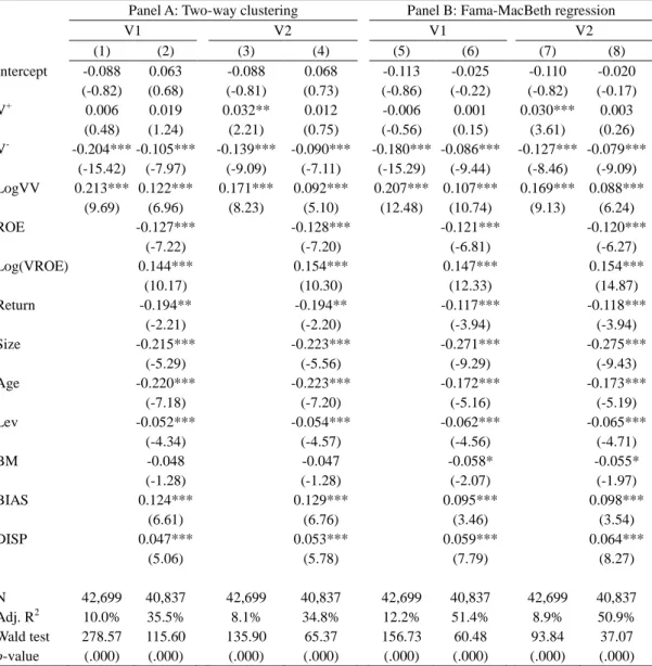
Table 3 presents estimated coefficients of the above regression, where total stock return volatility is the dependent variable. The t-statistics in parentheses are calculated using standard errors corrected for both clustering by firm and by year (Petersen 2009). The results support H1, indicating that future stock return volatility is significantly positively associated with the variability of current-period other information. The coefficients on VV are significant and positive in all specifications. For restricted estimates (Column (1) and (3)), the estimated coefficients are 0.213 (t = 9.69) for V1 and 0.171 (t = 8.23) for V2, indicating that a one standard deviation increase in the log of other information variance results in a more than 17% increase in the log of stock return volatility. When combined with all control variables (Column (2) and (4)), the magnitude of the slope coefficient of VV decreases to 0.122 (t = 6.96) and 0.092 (t = 5.10) but remains significant.
We then compare the effect of favorable versus unfavorable other information. There is a consistent negative association between volatility and V-. In column (1) and (3), for example, the regression coefficient is -0.204 for V1 (t = -15.42) and -0.139 for V2 (t = -9.09), suggesting a one standard deviation change in V- results in more than 14% change in future stock return volatility. However, the relationship between volatility and V+ is noticeably weaker. Although the estimated coefficient is statistically significant for V2 but not for V1 (0.006 for V1 with a t-value of 0.48 and 0.032 for V2 with a t-value of 2.21), its magnitude in both cases implies far lower economic significance. In fact, a one standard deviation increase in V+ results in less than a 3% increase in volatility. We use a Wald test with a null that β1 equals -β2 and find that the magnitude of the V- coefficient is significantly higher than that of the V+ coefficient. The above results do not alter substantially when all control variables are included. Thus the above results support H2, namely that stock return volatility tends to increase more in response to bad other information news than to good news.
Controlling for firm characteristics such as ROE and VROE does not change our conclusions, although the coefficients and robust t-statistics are attenuated (see columns (2) and (4)). The results confirm that other information variables provide incremental explanatory power of explaining future stock return volatility. In column (2), the regression coefficient on V- is -0.105, comparable to that for ROE (-0.127). The estimated coefficient on VV is 0.122, slightly lower than that for VROE (0.144). Most control variables have significant coefficients. ROE impacts negatively on future volatility, while VROE has a positive association. Small, young, and growth firms tend to be more volatile, as indicated by the significant and consistent signs of SIZE, AGE, and BM. The coefficients on BIAS and DISP are also consistent as hypothesized and statistically significant.
We also examine the robustness of our results to the Fama-MacBeth (1973) estimation and report the estimated coefficients in Panel B of Table 3.33 Comparing the results of Fama-MacBeth regressions to those in Panel A, the magnitude of the coefficients on other information variables declines slightly to -0.180 (V-) and 0.207 (VV) but still with significant t-statistics of -15.29 and 12.48 respectively (see column (5)). We also divide our sample period into three 10-year sub-periods, namely 1981-1990, 1991-2000, and 2001-2010 and estimate separately for the three subsamples. The results for different time periods are essentially the same and so are not reported in detail.34
[Insert Table 3 here]
4.2 Systematic volatility versus idiosyncratic volatility
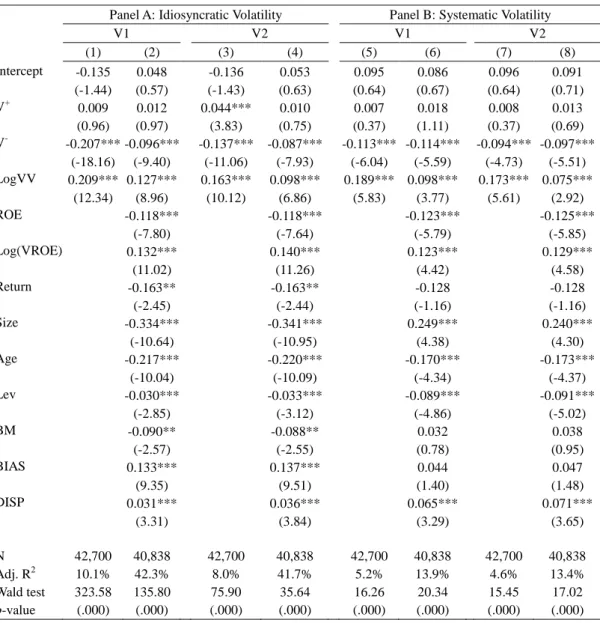
Our third hypothesis reflects the expectation that fundamental variables can cause both systematic and idiosyncratic variation in stock returns. Although it is widely held that most fundamental variables cause idiosyncratic volatility at the firm level, the relative importance of other information on systematic versus idiosyncratic volatility is ultimately an empirical issue. Table 4 presents the estimated coefficients for
33 The t-statistics reported in parentheses are adjusted for autocorrelation and conditional
heteroskedasticity (Newey and West 1987). The results of Fama-MacBeth regressions for other tables (untabulated) are similar to the results based on two-way clustering estimation.
34 We also employ a fixed effect regression to address possible concerns about unobserved individual
heterogeneity, where every firm and every year in the sample is assigned a dummy variable. The results (untabulated) are qualitatively similar to those reported above.