BGPE Discussion Paper
No. 83
Is There a Gap in the Gap?
Regional Differences in the Gender Pay Gap
Boris Hirsch
Marion König
Joachim Möller
October 2009
ISSN 1863-5733
Editor: Prof. Regina T. Riphahn, Ph.D.
Friedrich-Alexander-University Erlangen-Nuremberg © Boris Hirsch, Marion König, Joachim Möller
Is There a Gap in the Gap?
Regional Differences in the Gender Pay Gap
∗Boris Hirscha, Marion K¨onigb, Joachim M¨ollerc
Abstract: In this paper, we investigate regional differences in the gender pay gap both theoretically and empirically. Within a spatial oligopsony model, we show that more densely populated labour markets are more competitive and constrain employers’ ability to discriminate against women. Utilising a large administrative data set for western Germany and a flexible semi-parametric propensity score matching approach, we find that the unexplained gender pay gap for young workers is substantially lower in large metropolitan than in rural areas. This regional gap in the gap of roughly ten percentage points remained surprisingly constant over the entire observation period of thirty years.
Keywords: Gender pay gap, urban-rural differences, matching, monopsonistic discrimination
New JEL-Classification: J16, J42, J71
∗ We would like to thank Bernd Fitzenberger, Barbara Petrongolo, and Claus Schnabel for
their very useful suggestions. Furthermore, we appreciate helpful comments received from participants of the CEP labour market workshop and the economics research seminar at the Friedrich–Alexander–University Erlangen–N¨urnberg. Of course, all remaining errors are our own. Financial support of the Deutsche Forschungsgemeinschaft (DFG) through the research project MO523/41 “Flexibilit¨at der Lohnstruktur, Ungleichheit und Besch¨aftigung” within the “Schwerpunktprogramm 1169: Flexibilisierungspotenziale bei heterogenen Arbeitsm¨arkten” is gratefully acknowledged. The data used in this paper were made available by the Institute for Employment Research (IAB) at the Federal Employment Agency of Germany, N¨urnberg.
a Friedrich–Alexander–University Erlangen–N¨urnberg b University of Regensburg and IAB
c University of Regensburg, IAB, and IZA, corresponding author: Joachim M¨oller, Institute
for Employment Research, Regensburger Straße 104, D-90478 N¨urnberg, Germany, E-mail: [email protected]
1
Introduction
One of the most notable stylised facts in labour economics is that women earn substantially less than men. For instance, the European Commission (2006) reports an average raw wage differential of about 25 per cent for the EU-25 countries in 2002 and 26 per cent for Germany. While part of this gender pay gap is explained when introducing controls for individual characteristics (such as education, occupation, and experience), a substantial part of the gap remains unexplained in all EU-25 countries. In addition to reflecting differences in human capital or occupational segregation not controlled for, this unexplained part of the gap may also mirror discrimination against women.1 Although still of considerable size, the gender pay gap tends to narrow in most countries as in Germany over the last decades.2
While most of the empirical literature on the gender pay gap focusses on the variation of the gender pay gap between countries and its evolution over time, an aspect that has attracted far less attention is the regional variation of the gapwithin
the same country. Though many studies use regional information as control variables in the estimations, only few explicitly deal with its regional dimension. Blien and Mederer (1998), for instance, examine regional differences in the gender pay gap in Germany based on the wage curve approach, while McCall (1998) deals with the relation between regional restructuring and gender wage differentials in the U.S. For the UK, Phimister (2005) studies differences in urban wage premia by gender, while Robinson (2005) analyses the effect of the national minimum wage on the gender pay gap across regions. For Canada, Olfert and Moebis (2006) examine the different impact of rural and urban environments on gender occupational segregation. The two studies that are closest to our paper are Loureiroet al.(2004), who do not find regional differences in the gender pay gap in Brazil, and Busch and Holst (2008), who find lower gaps in cities than in rural areas in Germany in 2005.
However, to our knowledge, there has been made no attempt to systematically investigate regional differences in the gender pay gap and their evolution over time. What is more, there seems to be no economic theory around that readily explains
1 For a comprehensive review of the huge empirical literature on the gender pay gap, its
determinants, and its evolution over time, see Altonji and Blank (1999). Blau and Kahn (2003) investigate international differences in the gender pay gap for 22 countries between 1985–1994. Moreover, Weichselbaumer and Winter-Ebmer (2005) provide a large meta-analysis of more than 260 international studies between the 1960s and the 1990s. Finally, Maier (2007) provides a survey on the German literature.
2 While Maier (2007) arrives at the conclusion that the gap has remained rather stable during
the last decade, Blau and Kahn (2000) report a decreasing gap for West Germany and for almost all OECD countries up to the mid 1990s. Taking account of changes in the wage distributions as well as cohort and life cycle effects, Fitzenberger and Wunderlich (2002) find that the gap has narrowed substantially at the bottom of the wage distribution but to a lesser extent at the top. Using linked employer–employee data for Germany, Hinz and Gartner (2005) arrive at the conclusion that within-job pay gaps have shrunk as well.
why there should be such differences. The following paper is intended to fill these gaps.
The paper is organised as follows. Section 2 presents our theoretical considerations about the regional dimension of the gender pay gap and derives several hypotheses that will be tested in our empirical analysis. Section 3 lays out our empirical estimation strategy, while Section 4 describes the data set used. Our descriptive and multivariate empirical results are discussed in Sections 5 and 6, and Section 7 concludes.
2
Theory
2.1
Beckerian vs. Robinsonian Discrimination
Theoretical attempts of explaining discrimination often follow Becker’s (1971) concept of discrimination due to distaste. Since some employers dislike employing women, which is modelled by means of a distaste parameter in those employers’ utility function, they offer lower wages to women, ceteris paribus. Why should there be regional differences in the gender pay gap in this setting? One could argue that hot spots, i.e., large metropolitan areas, are trend-setters with more progressive environments and less discriminatory employers leading to less Beckerian discrimination. This kind of reasoning, however, suffers from several shortcomings (for details, see Madden, 1977b; Hirsch, 2009). In particular, Beckerian discrimination is costly for employers and should therefore be competed away in the long run if labour markets are sufficiently competitive. Furthermore, ‘[t]he attitudes which produce discriminatory behavior are taken as given. There is no consideration of whether the economic system fosters these attitudes.’ (Madden, 1977b, p. 102) Put drastically, this reasoning arrives at the conclusion of less discrimination in economic hot spots by just assuming it.
A different strand of literature employs a monopsonistic explanation of discrimination proposed by Robinson (1969), who applies Pigou’s (1932) concept of third-degree price discrimination to the labour market. Other than Beckerian discrimination, Robinsonian discrimination is not costly for firms the actions of which remain profit-maximising. In this setting, discriminating against women is simply the best firms can do. For this reason, it is more likely to survive in the long run. What is needed for Robinsonian discrimination to work, however, is that labour markets are imperfectly competitive and that firms face more monopsony power over their female than their male workers.
Hirsch (2009) presents a simple spatial duopsony model of the labour market in which workers are located at different places, while employers do not exist at each
potential location. Therefore, workers have to commute, facing some travel cost. Since employers and the jobs they offer are for this reason not perfect substitutes to workers, competition among employers is imperfect and firms possess some monopsony power. Assuming that women have higher average travel cost than men due to their domestic responsibilities, Hirsch arrives at the conclusion that firms have higher monopsony power over their female workers giving rise to a gender pay gap. In a nutshell, this holds because women are less mobile than men and thus less likely to change employers for wage-related reasons.3 Applying this reasoning, we shall
argue in the following that economic hot spots have thicker labour markets giving rise to a more competitive environment. And this higher degree of competition, in turn, not only pushes both female and male workers’ wages but also constrains employers’ ability to engage in Robinsonian discrimination. This will be formalised in the following within a model of spatial oligopsony in the tradition of Nakagome (1986) and Bhaskar and To (1999).
2.2
The Model
Workers’ Labour Supply Behaviour. Assume that equally productive workers’
homes are uniformly distributed along the real line at some density D. Firms demanding labour are located on the real line equidistantly, the distance between any two firms being some constantX. Workers supply a unit of labour wage-inelastically as long as they gain a positive income from working, so that they have a reservation income of zero. Moreover, a worker chooses the employer such that his or her income is maximised.
Next, suppose all workers face linear travel cost, that is, the worker’s travel cost is proportional to distance. This cost can be both direct and indirect. Direct cost results because travelling on its own is not costless, whereas indirect cost follows, for instance, from the fact that travelling requires time – and thus imposes opportunity costs – and that it might be uncomfortable to workers. Let t denote the travel cost per unit distance.
Consider now some firm, say firm i, and its two direct competitors, firms i−1 and i + 1, both distanced X from this firm. Firms are assumed to offer wages independently of workers’ location. Assume that firm i pays some wage w, while its competitors’ wage is ¯w. A worker distanced x, 06x6X, from firmihas travel cost tx to get to this firm and t(X −x) to get to firm i−1 or i+ 1, depending on which of these is nearer to the worker. The farther firm i, i.e., the larger x, the
3 There are alternative ways of modelling Robinsonian discrimination than spatial monopsony.
For an analysis of Robinsonian discrimination within a search model, see, for example, Schlicht (1982) and Bowlus (1997). Furthermore, Madden (1977b) investigates Robinsonian discrimination for segmented local labour markets.
higher is the worker’s travel cost to get to it and the lower is his or her travel cost to get to the respective competitor of firmi. Accordingly, the higher x, the more he or she prefers to work for firm i’s competitor.
A worker located at x receives an income of w− tx when working for firm i
and an income of ¯w−t(X −x) when working for the relevant competitor of firm
i. Therefore, he or she works for firm i as long as w−tx > w¯ −t(X −x) and for firm i’s competitor if the opposite holds as long as his or her income – i.e., the respective wage offer net of the travel cost – from doing so is positive; for otherwise the worker would choose not to work at all. Assume for the moment thatw+ ¯w > tX
holds, so that all workers decide to work. As we shall see later, this indeed holds in equilibrium under some mild parameter restrictions. The distancex∗ from firmi
at which a worker is indifferent between working for firm i and the relevant of its competitors, i.e., wherew−tx∗ = ¯w−t(X−x∗) holds, is given by
x∗ = w−w¯+tX
2t (1)
if |w−w¯|< tX.4 From this it follows that all workers distanced x < x∗ from firmi
prefer working for firmi and all of them distanced x > x∗ prefer working for one of its competitors.
From this reasoning it follows that firmi’s labour supply is given by
L(w,w¯) = 2Dx∗ = D(w−w¯+tX)
t . (2)
As a consequence, this model generates upward-sloping firm-level labour supply curves, although each individual worker supplies labour wage-inelastically at the level of the market (provided participation). The reason for this is that firm i is able to expand its market area and thus its labour supply at the expense of its rivals provided that it conjectures that its rivals do not react to a wage change, i.e.∂w/∂w¯ = 0. In the following, we will impose this familiar Bertrand–Nash assumption.
Firms’ Wage-Setting Behaviour. We now turn to firms’ decisions. Firms are
considered to behave as profit maximisers. We further assume that firms produce a homogenous good from their labour input with a constant marginal revenue product of labourφ.5 Finally, we assume that firms have to pay some fixed costs f to set up
4 If, on the other hand, |w−w¯|
> tX were to hold, either firm i or its competitors would not employ any workers. In a symmetric equilibrium, which we will derive, the condition |w−w¯|< tX of course holds.
5 It is straightforward to generalise this setting to the case with a second factor of production,
say capital, and a constant returns to scale production technology. In this case, we get a constant marginal revenue product of labour for each ratio of the output price and the capital rental rate due to the firm’s optimal adjustment of the capital stock employed (e.g., Bhaskar and To, 1999). Moreover, Bradfield (1990) shows that the (long-run) marginal revenue product
business. Therefore, firmi’s profits are given by
Π(w,w¯) = L(w,w¯)(φ−w)−f = D(w−w¯+tX)(φ−w)
t −f. (3)
Firmi’s problem is to find an optimal wage offerw that maximises its profits given its rivals’ wage offer ¯w, i.e., some w that solves the problem
max
w Π(w,w¯) =
D(w−w¯+tX)(φ−w)
t −f. (4)
In a symmetric equilibrium, the first-order condition of this problem, i.e.,
∂Π(w, w)/∂w = 0, can be used to obtain the firm’s optimal wage offer given some! fixed distance between firms X as
w(X) =φ−tX. (WSC)
We will refer to (WSC) as the wage-setting condition from now on. In the (X, w )-plane, (WSC) defines a straight line with slope w0(X) = −t and w-intercept φ. Two things are noteworthy: Firstly, if competition becomes fierce in the sense that there are many employers competing for workers, so that X is low, we approach the competitive solution, where workers get paid their marginal revenue product of labour. Second, if economic space becomes less densely populated by firms, so that
X increases, the wage chosen by the firms decreases because competitive forces are weakened.
Now consider what will happen if X is no longer fixed. This is achieved by allowing for free entry and costless relocation of firms. Free entry and costless relocation means that in the long run firms continue to enter (leave) the market until profits are driven to zero, so that the distance between equidistant firms X is endogenised.6 Setting Π(w, w) = 0, we get the distance between firms given some!
wagew as
X(w) = f
D(φ−w). (ZPC)
In the following, we will refer to (ZPC) as the zero-profit condition. In the (X, w
)-of labour is constant if the production technology inhibits constant returns to scale and there is perfect competition as well on all other factor markets than the labour market as on the firm’s output market.
6 In the following, we shall follow the literature in distinguishing the short run, where X is
some fixed value, from the long run, where X is pinned down to its zero-profit level (e.g., Capozza and Van Order, 1978; Salop, 1979; Greenhutet al., 1987). Note that by imposing the costless relocation assumption we guarantee the symmetric zero-profit equilibrium’s stability and suppress the whole adjustment process following competitive entry and exit. As Salop (1979, p. 145) states: ‘This equilibrium concept is static. In a dynamic context, it assumes that firms may costlessly relocate in response to entry and, in fact, do relocate. Thus, equal spacing is maintained.’
plane, (ZPC) defines an upward-sloping curve withX0(w) =f /[D(φ−w)2]>0 and
X-intercept f /Dφ. The higher is the wage w, the higher must be X to guarantee zero profits to the firms. Furthermore, we get a vertical line at X = 0 if the fixed costs tend to zero, so that we also approach the competitive solution if fixed costs disappear causing the setup of firms to be costless.
The Long-Run Equilibrium and Its Properties. Together (WSC) and (ZPC)
determine the symmetric Nash equilibrium under free entry. Combining both (WSC) and (ZPC) to solve for the long-run equilibrium wage, we obtain
w∗ =φ−
r f t
D. (5)
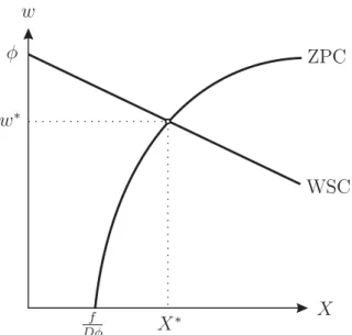
Obviously, ifφis sufficiently large,w∗ > tX∗/2 holds. Then, all workers are offered a positive income and thus decide to participate, and the equilibrium derived actually exists. The resulting symmetric zero-profit equilibrium can be depicted in the (X, w )-plane as the intersection point both of the wage-setting and the zero-profit curve (see Figure 1).
Figure 1: The symmetric zero-profit equilibrium (X∗, w∗).
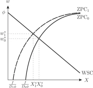
Now suppose we had two segmented labour markets, where the one labour market is more densely populated by workers, so that D1 > D0. Note that only the ZPC
is affected by changes in worker density, while they do not alter firms’ wage-setting behaviour. Put differently, the worker density only influences the labour market’s overall profitability, but has no impact on marginal decision-making. The ZPC’s intercept is shifted to the left, and the curve also becomes flatter. As a consequence, the interception point moves north-west on the WSC: w∗ rises and X∗ falls (see
Figure 2). Algebraically, we have ∂w∗/∂D > 0, which immediately follows from partial differentiation of (5). Intuitively, the higher worker density makes the labour market more profitable for firms, so that more firms enter the market. This reduces the distance between firms and therefore raises the competition among firms, so that the workers’ wage rises. Hence, the model predicts that workers earn higher wages in more densely populated labour markets.
Figure 2: The symmetric zero-profit equilibria (X0∗, w∗0) and (X1∗, w1∗) for worker densities D1 and D0 with D1 > D0.
In the next step, we adopt the idea presented and developed in Hirsch (2009) and assume that women face higher (average) travel cost than men,ceteris paribus. What might be reasons for different travel cost of men and women? We follow his argument that women have higher indirect travel cost because they (still) play a more exposed role in household production, particularly in rearing children, than men. So they attach a higher disutility to the time loss due to commuting, i.e., they face higher opportunity cost of travelling.7 The ceteris paribus clause in particular
means that we assume men and women to be perfect substitutes in production and to exhibit the same labour supply behaviour (i.e., they just decide on whether to participate having a reservation income of zero). Assume further that employers are free to offer wages separately to men and women, so that women and men supply
7 This is also in line with empirical evidence. For instance, Hersch and Stratton (1997) show
that for the U.S. married women’s housework time is, on average, three times that of married men’s and that women’s more dominant role in housework is able to explain part of the gender pay gap in wage regressions. Furthermore, Manning (2003, pp. 203/204) presents some evidence for the UK that travel-to-work times are lower for women than men, especially for those with more domestic responsibilities, while an older study by Madden (1977a) finds the same for women in the U.S. Finally, the Statistisches Bundesamt (2005, Appendix Table 29) reports a similar pattern for Germany. For a more complete discussion of the relation of gender differences in travel cost to the gender pay gap, see Hirsch (2009).
labour on segregated labour markets. Lett1 denote women’s andt0 men’s travel cost
per unit distance.
Note that only the WSC’s slope is affected by an increase in the travel cost. It becomes steeper. As a consequence, the interception point of WSC and ZPC moves south-west on the ZPC: Bothw∗ and X∗ fall (see Figure 3). Algebraically, we have
∂w∗/∂t <0, which follows at once from partial differentiation of (5). Intuitively, the higher travel cost reduces competition among firms because economic space – the source of firms’ wage-setting power in this framework – becomes more relevant in this segment of the labour market. And this, in turn, allows more firms to enter the labour market which has become more profitable for them. The model thus predicts that women should earn less than men, i.e., we have a long-run equilibrium gender pay gap. Women’s wage is lower because firms exploit the gender difference in the travel cost to exert third-degree wage discrimination.8
Figure 3: The symmetric zero-profit equilibria (X0∗, w∗0) and (X1∗, w∗1) for women’s travel costt1 and men’s travel cost t0 with t1 > t0.
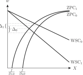
Finally, we are interested in the question whether the gender pay gap is higher or lower in more densely populated labour markets. Partially differentiating (5) gives ∂2w∗/∂D∂t > 0. That is, the higher the worker density D, the lower is the
gender wage differential ∆. Diagrammatically, this can be seen by combining the
8 One objection that could be raised against our reasoning is that in the long run women
may move, so that their firm-level labour supply becomes more elastic and discrimination cannot prevail. As argued by Hirsch (2009), however, in a dynamic model of monopsony the proportional gap between workers’ marginal revenue product and their wages is a weighted average of the inverse short-run and long-run firm-level labour supply elasticities, where the former’s weight is the firm’s discount factor. If thus workers, both men and women, move in the long run, so that the long-run elasticity tends to infinity for both groups, and firms discount future profits, women still get lower wages. The reason for this is simply their lower short-run elasticity which stems from their lower average short-term mobility.
two shifts from Figures 2 and 3 (see Figure 4): The wage differential in the more densely populated labour market ∆1 is smaller than the one in the less densely
populated ∆0 because the WSC in the female labour market is steeper than its
male counterpart. Furthermore, since wages are higher in more densely populated labour markets, this also implies that the gender pay gap ∆% is lower in these
labour markets. We thus get another prediction from the model: The gender pay gap should be higher in less densely populated labour markets. Intuitively, more densely populated labour markets are more profitable ones. This causes competitive entry of firms and therefore constrains employers’ monopsony power over both their female and male workers and also limits their ability to engage in Robinsonian discrimination.
Figure 4: The gender wage differentials ∆1 and ∆0 for segmented female and male
labour markets with worker densities D1 and D0 with D1 > D0.
2.3
Hypotheses
To sum up, our simple spatial oligopsony model delivers the following hypotheses: (1) We expect workers to earn higher wages in hot spots than in rural areas because
they have thicker labour markets with more competition among employers. (2) We conjecture female workers to earn lower wages, ceteris paribus, because of
their higher average (indirect) travel cost.
(3) Since we expect gender differences in the travel cost to have become less substantial over time (e.g., women have become more mobile relative to men due to more or better childcare facilities), we suspect the gender pay gap to decline over time as well.
(4) We expect the gender pay gap to be less pronounced in hot spots than in rural areas because the more competitive environment in hot spots constrains employers’ ability to engage in Robinsonian discrimination.
In the following empirical analysis, we will investigate to what extent these four hypotheses generated by the model are affirmed by the data and therefore check the model’s success in pattern prediction.9
3
Empirical Specification
Empirically, the raw gender wage differential is of limited information as it neglects individual heterogeneity, such as gender differences in the human capital endowment. In order to deal with observed heterogeneity, two approaches have been extensively used in the literature. The first approach is to estimate a standard Mincerian (1974) earnings function controlling for individual characteristics reflecting the worker’s productivity, such as education and experience, and including a female dummy as regressor. The coefficient of this dummy is then supposed to give theceteris paribus
gender pay gap that cannot be explained by differences in workers’ productivity. A second, more sophisticated approach, pioneered by Blinder (1973) and Oaxaca (1973), estimates two separate earnings functions for female and male workers and then decomposes the gender pay gap into an explained part due to different endowments in workers’ characteristics and an unexplained part. This well-known Oaxaca–Blinder decomposition and its extensions still serve as the backbone of the gender pay gap literature. In both approaches, the unexplained gender pay gap is typically attributed to discrimination (though gender differences in unobserved characteristics may also contribute to its explanation).
Using exact matching, ˜Nopo (2008) proposes another non-parametric approach to decompose the gender pay gap into an explained and an unexplained component.10
The intuitive idea of this empirical strategy is to use male workers with otherwise identical personal characteristics as a comparison group for females. That is, one compares the earnings of a female worker to the earning of male workers with the
9 Note that our model is highly stylised in some respects. For instance, workers’ labour
supply behaviour is modelled simplistically just as a ‘1–0 decision’ with all workers having a reservation income of zero and all workers participating in the equilibrium. It is, however, straightforward to extend the model, in a way following Bhaskar and To (1999), to allow for varying participation of workers. This can be achieved by incorporating some heterogeneity in reservation incomes, i.e., by considering groups of workers with different reservation incomes. While this would yield a positive relationship between workers’ wages and their participation rate – and thus, as a corollary to the gender pay gap, an equilibrium gender participation rate differential – the model’s other predictions would remain unaffected. Therefore, we will not consider this extension in detail.
10 Applications of this approach include Djurdjevic and Radyakin (2007) for Switzerland and
same observable characteristics.11 In analogy to the regression-based decomposition techniques, this approach allows to separate the endowment effect from the overall gender pay gap. The unexplained part is identified by taking the mean over the log gender wage differences of the matched female–male observations and is comparable to the unexplained part of the gender pay gap derived from an Oaxaca–Blinder decomposition based on female characteristics and evaluated at the male coefficients. Technically, the unexplained gender pay gap gained from this exact matching approach is the difference in expected earnings for female and male workers with the same observable characteristic, i.e.,
b E[∆%] = 1 C X x∈S b E[lnwi|x, di = 1]−E[lnb wj|x, dj = 0] c Pr[x|di = 1], (6)
where x is a row vector of observed characteristics, di a dummy variable taking on
the value one if individual i is female and zero otherwise, C the number of cells containing a given combination of covariates, andS the support of x.
With highly differentiated characteristics, however, the number of cells containing a given combination of covariates becomes prohibitive. Consequently, finding exact matches gets hard, and exact matching turns out to be not viable anymore. To flee this curse of dimensionality, the matching literature has followed Rosenbaum and Rubin (1983) in using the propensity score as a one-dimensional measure of similarity between individuals. In the context of gender pay gaps, Fr¨olich (2007) shows that propensity score matching can serve as a flexible semi-parametric approach to identify the unexplained part of the gap, where the appropriate propensity score is individuali’s fitted conditional probability of being female, i.e., Pr[cdi = 1|xi].
The main advantage of this semi-parametric approach is its flexibility. Other than the regression-based decomposition techniques, no functional form is imposed, apart from the specification of the propensity score. But misspecification of the earnings equation could yield misleading results. In particular, using observations where the empirical distributions of females’ and males’ characteristics substantially differ in their supports Sf and Sm could give biased results if the underlying ‘out-of-support’ assumption is invalid. As shown by Black et al. (2008) and ˜Nopo (2008), common support problems yield systematically upward-biased estimates of the unexplained part of the gender pay gap. Using a flexible semi-parametric propensity score matching approach and restricting to observations with a common support S =Sf ∩Sm, on the other hand, ensures that only those female and male
11 In terms of the program evaluation literature, the idea is to find male ‘statistical twins’ to
each female and to calculate the ‘average treatment effect on the treated’ (ATT) of being female. Of course, this would suggest an inappropriate causal interpretation of the ‘treatment’ sex. Notwithstanding, the basic principles of matching as a statistical approach to deal with heterogeneity in observable characteristics remain valid.
observations are matched that actually are comparable in terms of their observed characteristics.
In our empirical analysis, we arrive at individuals’ propensity score by fitting a probit model for their probability of being female, i.e., cPr[di = 1|xi] = Φ(xiβb)
with the estimated column vector of coefficients βb and the c.d.f. of the standard
normal distribution Φ. As matching variables we use a large number of individual characteristics. We include actual on-the-job experience and its square as well as tenure and its square as regressors. Furthermore, we add 13 dummies for occupation classes, four job position dummies, three dummies for pre-labour market education, seven establishment size dummies, a set of industry affiliation dummies, and a variable reporting the length of the employment per year.12 At this stage, it should be mentioned that lower gender pay gaps and higher wages in hot spots may feed back differently on female and male workers’ decision where to live and work. This, in turn, would introduce an endogeneity problem. To alleviate this problem we include a dummy for the type of region of first appearance on the labour market as additional matching variable. As a robustness check, we will also repeat the following analysis excluding those individuals who changed their type of region after their first appearance on the labour market.13
After fitting the propensity score, the next step is to choose a ‘similarity distance’ to match every female observation with comparable male observations based on the individual propensity score. For instance, n-nearest neighbour matching with replacement compares each female observation with its n nearest neighbours (in terms of their propensity score) among the male observations that lie in the common support S. For n = 1 we get nearest neighbour matching with replacement. The individual unexplained gender pay gap is then estimated as
b
∆%,i= lnwi−lnwj(i) (7)
wherej(i) is the nearest male observation in the common support, i.e.,
j(i) = argmin j|xj∈S cPr[di = 1|xi, di = 1]−Pr[cdj = 1|xj, dj = 0] (8)
with xi ∈ S. The expected unexplained gender pay gap in the sample is then
estimated simply as
12 Note that we cannot control for the worker’s marital status and number of children due to
data constraints, see footnote 17.
13 Unfortunately, we cannot control for endogenous migration between different types of regions
before individuals’ labour market entrance as we do not have such pre-labour market information.
b E[∆%] = 1 I I X i=1 b ∆%,i, (9)
whereI denotes the total number of matched females.
Of course, this is not the only way to form female–male matches. In the following, we will use nearest neighbour matching without replacement and kernel matching. While the prior uses every male observation only once and is therefore, arguably, the most restrictive procedure, kernel matching utilises all male observations within the common support for every female observation. It does so by attaching lower weights to more distant observations (in terms of their propensity score), where the weights follow from a kernel estimate of the characteristics distribution.14The corresponding
standard errors and confidence intervals are computed using bootstrapping with 100 replications. As a check of robustness, we will also apply the standard Oaxaca– Blinder decomposition technique.
To identify differences in the unexplained component of the gender pay gap between hot spots and rural areas, we will estimate E[∆%] for both types of regions
separately. Comparing the resulting estimates, we will argue that they differ if their bootstrapped confidence intervals do not overlap. But before we will put this into practice, we have to describe our data set used.
4
Data
In the following, we shall use social security data from the Institute for Employment Research (Institut f¨ur Arbeitsmarkt- und Berufsforschung, IAB). Our data set is the Regional File of the IAB Employment Samples (IAB-REG) which is a 2 per cent random sample from the employment register of Germany’s Federal Employment Agency (Bundesagentur f¨ur Arbeit).15 The German social security system requires
firms to record the stock of workers at least at the beginning and the end of each year. Additionally, all changes in employment relationships within the year (e.g., hirings, quits, and dismissals) have to be reported with the exact information on the date when the change occurred. Therefore, the employment register traces detailed histories for each worker’s time in covered employment as well as spells of unemployment for which the worker received unemployment benefits.16 This large
14 Since these two approaches can be regarded as the two ‘extremes’ of possible matching
procedures, it may be interesting to consider a somewhere-in-between procedure as well. Therefore, we will also apply three-nearest neighbour matching with replacement, results of which are reported in Appendix Figure A.1.
15 The data are briefly described in Bender et al. (2000) and in more detail in Bender et al.
(1996).
16 Episodes of unemployment during which the worker has no entitlement to unemployment
data set ranges from 1975 to 2004 and includes all workers, salaried employees, and trainees obliged to pay social security contributions. All in all, it covers more than 80 per cent of all those employed. Since they are not covered by social security, civil servants, family workers, and self-employed are not included. As misreporting leads to sanctions for the employer, the information on periods of coverage and earnings is highly reliable.
The data include, among others thing, information for every employee on the daily gross wage, censored at the social security contribution ceiling, on several individual, and on some establishment characteristics. Characteristics contained are, among others, the worker’s age, skill level, sex, job status, occupation, and nationality and the employer’s industry, location at the district level, and establishment size.17 Not included, however, is a variable with quantitative information on the hours worked. Although the data set comprises a qualitative variable distinguishing between full-time and two sorts of part-time work, this limits the information value of the daily gross wages contained in the data because we cannot infer workers’ wage rates from them. Hence, we restrict our sample to individuals working full time in order to account for the problem of missing working hours information.18
In the following empirical analysis, we only consider individuals in western Germany who are employed full time on the 30th of June in each year. Additionally, we exclude part-time workers, home workers, trainees, and spells of minor employment. Since we argue that new social trends and especially changes in gender mobility patterns are first visible for entrants in the labour market and young workers, we restrict our sample to individuals between 25 and 34 years old. The lower bound ensures that most individuals have completed their education. Furthermore, the upper bound additionally alleviates a problem with the wage data, viz., daily gross wages are censored at the social security contribution ceiling. Since this censoring problem bites only for high-wage observations, we exclude high-skilled workers, i.e., workers with higher education (Abitur, which is the German equivalent to A-levels or graduation from high school) and a completed vocational training or with a university type of education. Together, the age restriction and the exclusion
in the labour market.
17 Unfortunately, the data include information on the worker’s marital status and number of
children only due to notifications made in the case of changes in employment that are relevant according to benefit entitlement rules. Using this information would clearly introduce a severe selectivity problem. Consequently, we will not be able to use it in the following analysis.
18 One might argue that higher daily earnings of male workers could be the consequence of gender
differences in hours worked. Restricting to full-time employees again alleviates this potential problem. Moreover, this explanation would be at odds with differences in the gender pay gap between hot spots and rural areas because taking differences should eliminate this working hours effect (provided the gender distribution of working hours is sufficiently similar between full-time workers in the two types of regions).
of high-skilled workers minimise the problem of censored wages as the number of top-coded observations in our sample is negligible.19
We are aware of possible job instability for female workers. Therefore, we constructed a series of actual rather than potential experience on the job, where only periods of active employment are counted.20 In a similar way, a measure of
tenure is calculated as the total time period worked within the same firm.
Another limitation in the data set is that, despite a high precision for the earnings variable, information on personal characteristics might suffer from reporting errors. This could especially affect the skill variables. Several attempts have been made to correct the qualification information contained in IAB-REG, most notably the widely applied approach by Fitzenberger et al. (2006). Notwithstanding, we will follow a different route here: For most observations the data cover the complete training, employment, and unemployment history. Therefore, the individual skill level can be checked by taking all these spells into account. We apply the following procedure: Cases where the skill level is almost unambiguous according to the employment histories are used to fit a logit model for the conditional probability of having a certain skill level. In a next step, using the model’s estimated coefficients, this probability is predicted for the ‘uncertain’ cases given the full set of information on the individual’s employment history. Finally, we scan the whole employment history for each individual including the imputed skill level formed from the results of the logit estimations in order to check for consistency and to correct the qualifications accordingly.
Eventually, for the assignment of districts to rural areas and hot spots we use a classification scheme developed by the German Federal Office for Building and Regional Planning (Bundesamt f¨ur Bauwesen und Raumordnung, BBR). This scheme distinguishes between areas with large agglomerations, areas with features of conurbation, and areas of rural character, each of these again being subdivided into different groups. All in all, it differentiates between nine types of regions (districts) at the NUTS (nomenclature des unit´es territoriales statistiques) 3 level according to their population density and accessibility. We define economic hot spots as western Germany’s eight biggest metropolitan areas: Cologne, Dortmund, D¨usseldorf, Essen, Frankfurt, Hamburg, Munich, and Stuttgart. All hot spots are metropolitan core cities (BBR type 1). Asrural areas we choose all districs with BBR types 7 to 9 (see Figure 5).21
19 In our sample, only 2.5 per cent of all observations contain censored wages. This number is
slightly higher for men (3.3 per cent) than for women (0.9 per cent) and also for hot spots (4.3 per cent) than for rural areas (0.9 per cent).
20 Note, however, that for observations prior to the end of the 1980s the measure of actual
experience might be biased due to left censoring of employment spells in the data.
21 BBR type 7 consists of rural districts in regions with intermediate agglomeration. BBR type 8
Hamburg Dortmund Essen Düsseldorf Cologne Frankfurt Stuttgart Munich
Notes:Hot spots are defined as the eight biggest metropolitan areas in western Germany coloured in black. The gray areas display the rural areas characterised by BBR types 7 to 9.
Figure 5: Hot spots and rural areas.
5
Descriptive Evidence
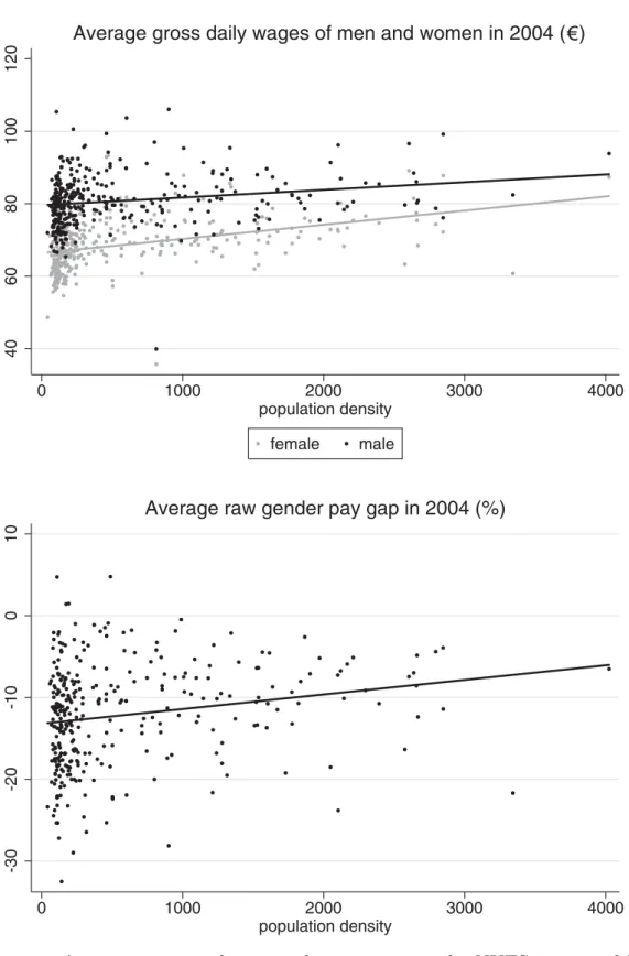
First of all, we present some descriptive evidence. The upper graph in Figure 6 shows a scatter plot of average gross daily wages of full-time employed young females and males of the 327 western German NUTS 3 regions in 2004 and the population density per region (measured as population per square kilometre) including trend lines. Three things are noteworthy: Firstly, the average wage is rising in the population density both for males and females. This is in line with our first hypothesis that workers earn higher wages in more densely populated labour markets. Second, the average wage is higher for males than for females and thus points at a gender pay gap, our second hypothesis. Third, the trend line for females appears to be steeper than that for males. This level effect points at a lower wage differential in hot spots than in rural areas and therefore, in particular, at a lower gender pay gap. In the lower graph in Figure 6, we see that the average raw gender pay gap is indeed decreasing (in absolute value) in the population density. Put differently, when not
€
Figure 6: Average wages and raw gender pay gaps at the NUTS 3 regional level by population density (the respective solid lines are trend lines resulting from a univariate regression).
controlling for individual characteristics, the gap is more pronounced in rural areas than in cities. This is consistent with our fourth hypothesis that the gender pay gap should be lower in hot spots.
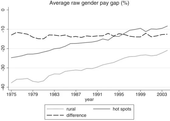
Figure 7 shows the evolution of the average raw gender pay gaps in hot spots and rural areas from 1975 to 2004. It is worth mentioning that both gaps are substantially declining over time by almost 16 percentage points. While women in rural areas (hot spots) earned on average about 38 per cent (25 per cent) less than men in 1975, this pay gap has narrowed to 22 per cent (9 per cent) in 2004. What is more, the difference in the gaps between hot spots and rural areas remained strikingly stable during this long period of time, oscillating around 13 percentage points. While the reduction in the gaps in both hot spots and rural areas are in line with our third hypothesis of declining gender pay gaps over time, the latter finding is consistent with our fourth hypothesis at the heart of this paper, viz., that the gender pay gap should be lower in hot spots than in rural areas.
Figure 7: Average raw gender pay gaps in hot spots and rural areas 1975–2004.
6
Multivariate Evidence
While it is reassuring to see that there is supportive descriptive evidence to all our hypotheses, we now turn to our multivariate results. As laid out in detail in Section 3, we will in the following present estimates gained from a semi-parametric propensity score matching approach to the unexplained part of the gender pay gap as put forward by Fr¨olich (2007). We used both nearest neighbour matching without replacement and kernel matching as the most and least restrictive methods in terms of the number of male observations used to create a ‘synthetic’ male
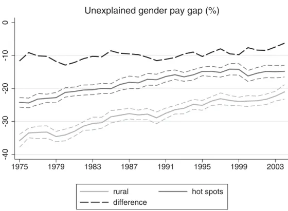
comparison observation for each female observation in the common support of observed characteristics.22 For each of the years 1975 to 2004 we estimate the unexplained gender pay gap in both hot spots and rural areas employing nearest neighbour and kernel matching. The corresponding standard errors and confidence intervals are calculated using bootstrapping with 100 replications. The results obtained from nearest neighbour matching are shown in Figure 8, those obtained from kernel matching in Figure 9, where the thin dashed lines represent the respective 95 per cent confidence bands. Since the results of both approaches are very similar, we shall discuss them simultaneously.23
First of all, our second hypothesis is clearly confirmed. Young full-time employed females earn significantly less than males with the same (observed) characteristics. This even holds after controlling for experience, tenure, education, job position, occupation, establishment size, industry, length of employment, and region of first entrance in the labour market.24 And this is valid both in economic hot spots and
rural areas.
Second, while this unexplained pay gap narrowed considerably in both types of regions during our observation period, it is still of substantial size. In the mid-1970s, it was about 35 per cent (25 per cent) in rural areas (hot spots) and only 22 per cent (15 per cent) at the beginning of the new millennium. This gradual decline is highly supportive to our third hypothesis. Moreover, this strikingly parallel development in both types of regions points at our next finding.
Third, and most importantly, there is a considerable difference between rural areas and hot spots. In each of the 30 years considered, the gender pay gap is smaller in hot spots than in rural areas. While this difference is statistically significant throughout, it is also economically significant: The gender pay gap is about 10 percentage points lower in hot spots than in rural areas. What is more, this difference is remarkably stable over time (with a small decline in the point
22 Since nearest neighbour matching without replacement uses male observations only once to
form a comparison observation for females, there were clearly more female observations where no male could be matched than with the other matching methods. In this case, the results are only valid for the matched individuals. On the other hand, the resulting matched female–male observations were highly balanced with indistinguishable observed characteristics in nearly all cases, while this balancing property was satisfied to a lesser degree by the samples obtained from the less restrictive matching methods. Since results proved to be highly robust across specifications, we conclude that neither the absence of perfect balancing nor external validity seems to be a problem.
23 Note that basically the same results are found when using three nearest neighbour matching
with replacement, results of which are shown in Appendix Figure A.1.
24 Note that this unexplained pay gap may not only be due to discrimination but also due
to differences in unobserved characteristics which we cannot control for. Therefore, this unexplained gap is likely to overestimate the impact of discrimination. Though one could argue that differences in unobservables would net out when taking differences between the two types of region if unobservables were equally distributed between hot spots and rural areas, we will not do so as this seems to be a far-fetched assumption in our eyes.
Figure 8: Unexplained gender pay gaps in hot spots and rural areas 1975–2004 using nearest neighbour matching without replacement (the thin dashed lines represent the respective 95 per cent confidence bands).
Figure 9: Unexplained gender pay gaps in hot spots and rural areas 1975–2004 using kernel matching (the thin dashed lines represent the respective 95 per cent confidence bands).
estimate in the two last years of observation) and therefore clearly affirms our fourth hypothesis.
Figure 10: Unexplained gender pay gaps in hot spots and rural areas 1975– 2004 using the Oaxaca–Blinder decomposition (the thin dashed lines represent the respective 95 per cent confidence bands).
Basically, the same picture arises when applying the standard Oaxaca–Blinder decomposition technique (with females as reference group) results of which are shown in Figure 10. The same also holds when only those individuals are included in the analysis who stayed in the same regional type of first appearance in the labour market (see Appendix Figure A.2). As argued above, this robustness check indicates that the endogeneity problem arising because individuals can choose to live and work in a hot spot is only of minor importance in this context.25
All in all, our very robust empirical findings strongly corroborate the four hypotheses derived from our theoretical model. Firstly, workers’ wages are higher
25 Note that also a sample selection problem may arise due to the participation decisions
of women. A possible solution would be to take these participation decisions explicitly into account and to apply Heckman’s (1979) two-stage procedure. Our data set, however, does not contain a personal characteristic that could serve as a reliable instrument for women’s participation decision. As argued by Olivetti and Petrongolo (2008), however, if non-participation is non-random and participating women therefore have more favourable characteristics, then differences in the gender pay gap may be explained by differences in the participation gap. In our sample, the participation rate of females is almost identical in hot spots and rural areas (69 vs. 70 per cent), as is the female full-time employment ratio (44 vs. 43 per cent). Therefore, it seems implausible that our results are driven by participation differences, whereas the initial sample selection problem is likely to net out when considering the hot spot–rural difference in the pay gaps.
in more densely populated areas. Second, women earn significantly less than comparable men both in hot spots and rural areas. Third, the unexplained gender pay gap is decreasing over time in both types of regions. Fourth, the gap is significantly lower in hot spots than in rural areas. Strikingly, our main finding is that this hot spot–rural difference in the pay gap is almost constant over the entire period of 30 years without any sign of a catching-up process.
7
Conclusions
In this paper, we have investigated regional differences in the gender pay gap between hot spots and rural areas for young full-time workers and their evolution over time using a large micro data set from western Germany ranging from 1975– 2004. Our empirical results strongly support the hypotheses generated from a spatial oligopsony model where women are less mobile due to more domestic responsibilities. According to this model, hot spots have thick labour markets giving rise to a more competitive environment. This not only pushes wages in hot spots but also constrains employers’ ability to engage in monopsonistic Robinsonian discrimination. Other than under Beckerian discrimination due to distaste, firms do not forego profits when discriminating against women. Robinsonian discrimination is therefore more likely to survive in the long run and represents in our eyes a more convincing economic explanation of the gender pay gap.
In our empirical analysis, we used a semi-parametric propensity score matching approach to identify the unexplained part of the gender pay gap. Other than the standard regression-based decomposition techniques, such as the Oaxaca–Blinder decomposition, this technique is more flexible in terms of the imposed functional form and does not rely on an ‘out-of-support’ assumption, i.e., it compares only female and male observations with characteristics in their common support.
Our main result is that the unexplained gender pay gap is about 10 percentage points larger in rural areas compared to hot spots. While the unexplained gap both in hot spots and rural areas gradually decreases over time, the hot spot–rural difference remains astonishingly stable. To the best of our knowledge, this is the first paper to investigate and find such a stable difference over a long period of time. In the context of our model, the interpretation of these findings would be that the gender difference in mobility gradually shrank over time, leading to a decrease in the gender pay gaps, whereas the different competitive environment in hot spots and rural areas persisted. That is to say, labour markets of hot spots remained more competitive with more firms in them, limiting employers’ ability to discriminate against women.
References
Altonji, J.G. and Blank, R.M. (1999), ‘Race and gender in the labor market,’
in O.C. Ashenfelter and D.E. Card (eds.), ‘Handbook of Labor Economics,’ vol. 3C, pp. 3143–3259, Amsterdam: Elsevier.
Becker, G.S. (1971), The Economics of Discrimination, Chicago, IL: University
of Chicago Press, 2nd edn.
Bender, S.,Haas, A., and Klose, C. (2000), ‘The IAB employment subsample
1975–95,’ Schmollers Jahrbuch (Journal of Applied Social Science Studies),
120(4):649–662.
Bender, S., Hilzendegen, J., Rohwer, G., and Rudolph, H. (1996),
Die IAB-Besch¨aftigtenstichprobe 1975–1990, Beit¨age zur Arbeitsmarkt-und Berufsforschung Nr. 197, N¨urnberg: Institut f¨ur Arbeitsmarkt- und Berufsforschung.
Bhaskar, V. and To, T. (1999), ‘Minimum wages for Ronald McDonald
monopsonies: A theory of monopsonistic competition,’ Economic Journal,
109(455):190–203.
Black, D.A., Haviland, A.M., Sanders, S.G., and Taylor, L.J. (2008),
‘Gender wage disparities among the highly educated,’ Journal of Human Resources, 43(3):630–659.
Blau, F.D. and Kahn, L.M. (2000), ‘Gender differences in pay,’ Journal of
Economic Perspectives, 14(4):75–99.
——— (2003), ‘Understanding international differences in the gender pay gap,’
Journal of Labor Economics, 21(1):106–144.
Blien, U. and Mederer, A. (1998), ‘Regional determinants of gender specific
wages – an empirical analysis,’ in F. Haslinger and O. St¨onner-Venkatarama (eds.), ‘Aspects of the Distribution of Income,’ pp. 273–295, Marburg: Metropolis.
Blinder, A.S. (1973), ‘Wage discrimination: Reduced from and structural
estimates,’Journal of Human Resources, 8(4):435–455.
Bowlus, A.J. (1997), ‘A search interpretation of male–female wage differentials,’
Journal of Labor Economics, 15(4):625–657.
Bradfield, M. (1990), ‘Long-run equilibrium under pure monopsony,’ Canadian
Busch, A.and Holst, E.(2008), ‘“Gender Pay Gap”: In Großst¨adten geringer als auf dem Land,’DIW Wochenbericht, 75(33):462–468.
Capozza, D.R. and Van Order, R. (1978), ‘A generalized model of spatial
competition,’American Economic Review, 68(5):896–908.
Djurdjevic, D.andRadyakin, S.(2007), ‘Decomposition of the gender wage gap
using matching: An application from Switzerland,’Swiss Journal of Economics and Statistics, 143(4):365–396.
European Commission (2006), The Gender Pay Gap – Origins and Policy
Responses: A Comparative Review of 30 European Countries, Luxembourg: European Commission.
Fitzenberger, B.,Osikominu, A., andV¨olter, R.(2006), ‘Imputation rules to
improve the education variable in the iab employment subsample,’ Schmollers Jahrbuch (Journal of Applied Social Science Studies), 126(3):405–436.
Fitzenberger, B. and Wunderlich, G. (2002), ‘Gender wage differentials in
West Germany: A cohort analysis,’German Economic Review,3(4):379–414.
Fr¨olich, M.(2007), ‘Propensity score matching without conditional independence
assumption – with an application to the gender wage gap in the United Kingdom,’Econometrics Journal, 10(2):359–407.
Greenhut, M.L., Norman, G., and Hung, C.S. (1987), The Economics of
Imperfect Competition: A Spatial Approach, Cambridge: Cambridge University Press.
Heckman, J.J. (1979), ‘Sample selection bias as a specification error,’
Econometrica,47(1):153–161.
Hersch, J. and Stratton, L.S. (1997), ‘Housework, fixed effects, and wages of
married women,’ Journal of Human Resources, 32(2):285–307.
Hinz, T. and Gartner, H. (2005), ‘Geschlechtsspezifische Lohnunterschiede in
Branchen,’ Zeitschrift f¨ur Soziologie, 34(1):22–39.
Hirsch, B. (2009), ‘The gender pay gap under duopsony: Joan Robinson meets
Harold Hotelling,’ Scottish Journal of Political Economy, forthcoming.
Loureiro, P.R.A.,Carneiro, F.G., andSachsida, A.(2004), ‘Race and gender
discrimination in the labor market: An urban and rural sector analysis for Brazil,’ Journal of Economic Studies, 31(2):129–143.
Madden, J.F. (1977a), ‘An empirical analysis of the spatial elasticity of labor supply,’Papers in Regional Science, 39(1):157–171.
——— (1977b), ‘A spatial theory of sex discrimination,’Journal of Regional Science,
17(3):369–380.
Maier, F. (2007), The Persistence of the Gender Wage Gap in Germany,
Harriet Taylor Mill–Institut f¨ur ¨Okonomie und Geschlechterforschung, Berlin, Discussion Paper 12/2007.
Manning, A. (2003), Monopsony in Motion: Imperfect Competition in Labor
Markets, Princeton, NJ: Princeton University Press.
McCall, L. (1998), ‘Spatial routes to gender wage (in)equality: Regional
restructuring and wage differentials by gender and education,’ Economic Geography, 74(4):379–404.
Mincer, J. (1974), Schooling, Experience, and Earnings, New York: National
Bureau of Economic Research.
Nakagome, M. (1986), ‘The spatial labour market and spatial competition,’
Regional Studies, 20(4):307–312. ˜
Nopo, H. (2008), ‘Matching as a tool to decompose wage gaps,’ Review of
Economics and Statistics, 90(2):290–299.
Oaxaca, R.L. (1973), ‘Male–female wage differentials in urban labor markets,’
International Economic Review, 14(3):693–709.
Olfert, R.M.and Moebis, D.M. (2006), ‘The spatial economy of gender-based
occupational segregation,’ Review of Regional Studies,36(1):44–62.
Olivetti, C.andPetrongolo, B.(2008), ‘Unequal pay of unequal employment?
A cross-country analysis of gender gaps,’ Journal of Labor Economics,
26(4):621–654.
Phimister, E.(2005), ‘Urban effects on participation and wages: Are there gender
differences?’Journal of Urban Economics,58(3):513–536.
Pigou, A.C. (1932),The Economics of Welfare, London: Macmillan, 4th edn.
Robinson, H. (2005), ‘Regional evidence on the effect of the national minimum
wage on the gender pay gap,’Regional Studies,39(7):855–872.
Robinson, J.V. (1969), The Economics of Imperfect Competition, London:
Rosenbaum, P.R. and Rubin, D.B. (1983), ‘The central role of the propensity score in observational studies of causal effects,’Biometrika,70(1):41–55.
Salop, S.C. (1979), ‘Monopolistic competition with outside goods,’ Bell Journal
of Economics, 10(1):141–156.
Schlicht, E. (1982), ‘A Robinsonian approach to discrimination,’ Zeitschrift
f¨ur die Gesamte Staatswissenschaft (Journal of Institutional and Theoretical Economics),138(1):64–83.
Statistisches Bundesamt (2005), Leben und Arbeiten in Deutschland,
Wiesbaden: Statistisches Bundesamt.
Weichselbaumer, D. and Winter-Ebmer, R. (2005), ‘A meta-analysis of the
international gender wage gap,’Journal of Economic Surveys,19(3):479–511.
Appendix
Figure A.1: Unexplained gender pay gaps in hot spots and rural areas 1975–2004 using three-nearest neighbour matching with replacement (the thin dashed lines represent the respective 95 per cent confidence bands).
Figure A.2: Unexplained gender pay gaps in hot spots and rural areas 1975– 2004 using only individuals without change of regional type of first appearance in the labour market and three-nearest neighbour matching with replacement (the thin dashed lines represent the respective 95 per cent confidence bands).