of cDNA microarray experiment
Ximin Zhu
A Dissertation Submitted to the University of Glasgow
for the degree of Doctor of Philosophy
Department of Statistics
May 2009
c
A microarray is a powerful tool for surveying the expression levels of many thou-sands of genes simultaneously. It belongs to the new genomics technologies which have important applications in the biological, agricultural and pharmaceutical sciences.
In this thesis, we focus on the dual channel cDNA microarray which is one of the most popular microarray technologies and discuss three different topics:
• Optimal experimental design,
• Estimating the true proportion of true nulls, local false discovery rate (lFDR) and positive false discovery rate (pFDR),
• Dye effect normalization.
The first topic consists of four subtopics each of which is about an indepen-dent and practical problem of cDNA microarray experimental design. In the first subtopic, we propose an optimization strategy which is based on the simulated annealing method by Wit et al. (2005) to find optimal or near-optimal designs with both biological and technical replicates. In the second subtopic, we discuss how to apply Q-criterion for the factorial design of microarray experiments. In the third subtopic, we suggest an optimal way of pooling samples, which is actu-ally a replication scheme to minimize the variance of the experiment under the
proper and propose an alternative criterion instead.
The second topic of this thesis is dye effect normalization. For cDNA microar-ray technology, each armicroar-ray compares two samples which are usually labelled with different dyes Cy3 and Cy5. It assumes that: for a given gene (spot) on the array, if Cy3-labelled sample has k times as much of a transcript as the Cy5-labelled sample, then the Cy3 signal should be k times as high as the Cy5 signal, and vice versa. This important assumption requires that the dyes should have the same properties. However, the reality is that the Cy3 and Cy5 dyes have slightly different properties and the relative efficiency of the dyes vary across the intensity range in a “banana-shape” way. In order to remove the dye effect, we propose a novel dye effect normalization method which is based on modeling dye response functions and dye effect curve. Real and simulated microarray data sets are used to evaluate the method. It shows that the performance of the proposed method is satisfactory.
The focus of the third topic is the estimation of the proportion of true null hypotheses, lFDR and pFDR. In a typical microarray experiment, a large number of gene expression data could be measured. In order to find differential expressed genes, these variables are usually screened by a statistical test simultaneously. Since it is a case of multiple hypothesis testing, some kind of adjustment should be made to the p-values resulted from the statistical test. Lots of multiple test-ing error rates, such as FDR, lFDR and pFDR have been proposed to address this issue. A key related problem is the estimation of the proportion of true null hypotheses (i.e. non-expressed genes). To model the distribution of the p-values, we propose three kinds of finite mixture of unknown number of components (the
method called allocation sampler to estimate the proportion of true null (i.e. the mixture weight of the first component). The method also provides a framework for estimating lFDR and pFDR. Two real microarray data studies plus a small simulation study are used to assess our method. We show that the performance of the proposed method is satisfactory.
I would like to take this opportunity to thank everyone who has supported me throughout the completion of this thesis.
Firstly, I would like to thank my supervisors Dr. Agostino Nobile and Prof. Ernst Wit, who contributed their time, expertise to this thesis. I would also like to thank my second supervisor Prof. Marian Scott for her very important help during my PhD studies. Thanks must also go to all the other members of the statistics department who have helped make the last few years a enjoyable experience. I am very grateful for all the opportunities the department gave me. Also, I must thank the Overseas Research Students (ORS) Awards Scheme for funding me throughout this PhD studies.
Finally, I am very grateful to my family and all my friends for all they have done for me over the years. I must thank my parents and my wife for their love, support and encouragement through both good and hard times.
This thesis has been composed by myself and it has not been submitted in any previous application for a degree. The work reported within was executed by myself, unless otherwise stated.
May 2009
Abstract i
Acknowledgements iv
1 Introduction 1
2 Optimal design of cDNA microarray experiments 7
2.1 Introduction to cDNA microarray experimental design . . . 7
2.1.1 Microarray experimental effects . . . 8
2.1.2 Replication . . . 11 2.1.3 Pooling . . . 13 2.1.4 Experimental designs . . . 14 2.1.4.1 Direct comparisons . . . 14 2.1.4.2 Reference design . . . 17 2.1.4.3 Loop design . . . 18
2.1.4.4 Interwoven loop design . . . 19
2.1.4.5 Alternative designs . . . 20
2.2 Optimal design with biological and technical replicates . . . 21
2.2.1 A statistical model for microarray gene expression intensity 21 2.2.2 Parametrization and estimation . . . 23
2.2.5 Simulated annealing implementation for finding near-optimal
designs . . . 30
2.2.6 Results . . . 34
2.2.6.1 Example one . . . 34
2.2.6.2 Example two . . . 37
2.2.6.3 Are dye-swap designs optimal? . . . 38
2.3 Optimal design for factorial experiment . . . 40
2.3.1 Statistical gene expression models forp×q factorial exper-iment . . . 41
2.3.2 Q-criterion . . . 42
2.3.3 Simulated annealing implementation for finding near Q-optimality design . . . 44
2.3.4 An example: 2×4 factorial microarray experiment . . . . 45
2.3.5 Conclusion . . . 48
2.4 Optimal pooling strategy . . . 50
2.4.1 Methods . . . 50
2.4.2 Example . . . 55
2.5 Optimal distant pair design . . . 57
2.5.1 Introduction . . . 57
2.5.2 Model . . . 59
2.5.3 Optimality criteria . . . 61
2.5.4 Example . . . 61
3 Dye effect normalization 68
3.1.2 Dye effect normalization methods . . . 73
3.1.2.1 Dye swap method . . . 73
3.1.2.2 ANOVA method . . . 73
3.1.2.3 Two-step intensity-dependent dye normalization method . . . 74
3.2 Method . . . 80
3.2.1 Dye response model . . . 80
3.2.1.1 Model one . . . 81
3.2.1.2 Model two . . . 90
3.3 Results . . . 96
3.3.1 Evaluating the model . . . 97
3.3.2 Evaluating the method . . . 97
3.4 Discussion . . . 108
4 Estimating the proportion of true nulls 110 4.1 Introduction . . . 110
4.2 Multiple hypothesis testing and error rates . . . 113
4.2.1 Classical hypothesis testing . . . 113
4.2.2 Multiple hypothesis testing . . . 115
4.2.3 Error rates for multiple testing . . . 116
4.2.3.1 False positive rate (FPR) . . . 117
4.2.3.2 Family-wise error rate (FWER) . . . 117
4.2.3.3 FWER controlling procedures . . . 118
4.2.3.4 False discovery rate (FDR) . . . 119
4.2.3.7 Positive false discovery rate (pFDR) . . . 123
4.2.3.8 Local FDR (lFDR) . . . 125
4.3 The mixture model and the estimate of the proportion of true nulls 127 4.3.1 The two-component mixture model for the distribution of the test statistic . . . 127
4.3.2 Motivation for estimatingπ0 . . . 127
4.3.3 The two-component mixture model for the distribution of p-values . . . 128
4.3.4 Some recent methods for estimating π0 . . . 128
4.4 The proposed mixture models with an unknown number of com-ponents . . . 134
4.4.1 Model 1: The uniform mixture distributions . . . 134
4.4.2 Model 2: The one-parameter beta mixture distributions . 135 4.4.3 The inference problem . . . 136
4.5 A Bayesian approach for finite mixture model . . . 137
4.5.1 Introduction . . . 137
4.5.2 The allocation sampler . . . 140
4.5.2.1 Calculating f(g|k) . . . 141
4.5.2.2 Calculating f(x|k, g, φ) . . . 142
4.5.2.3 Application to Model 1: The uniform mixture dis-tributions . . . 143
4.5.2.4 Application to Model 2: The one-parameter beta mixture distributions . . . 146
4.5.2.5 Posterior distributions . . . 147
4.6.1 Allocation sampler procedure . . . 152
4.6.2 Breast cancer data . . . 153
4.6.3 Lipid metabolism data . . . 161
4.6.4 A small simulation study . . . 164
4.7 Discussion . . . 172
5 Conclusion and future research 175 A Computing Σ 181 B Integrating parameters from the model 185 B.1 Uniform distribution . . . 185
B.2 One-parameter Beta distribution . . . 187
C Calculate true pFDR and lFDR 190
2.1 A Latin Square design to compare two samples directly. . . 15 2.2 The elements of weight matrix W = {wij}i,j=0,...,7 are computed
for 2×4 factorial design. Note that i and j denote the index of two effects in the maximal model respectively, and wij = wji, for
i6=j. . . 48 2.3 The corresponding xi1 and xi2 values are listed for the 16 possible
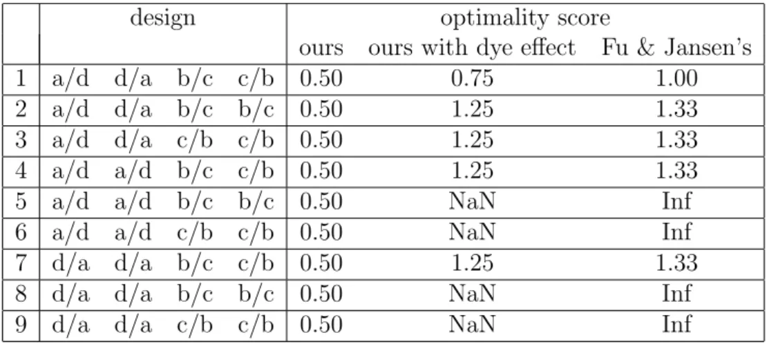
combinations from the four types of RILsa,b, cand d. . . 62 2.4 The 9 optimal designs found by our A-optimality criterion (dye
ef-fect excluded) and also their corresponding optimality scores under our criterion (dye effect included) and Fu & Jansen’s criterion. . 66 2.5 The 3 optimal designs found by Fu & Jansen’s criterion and also
their corresponding optimality scores under our criteria (dye effect ignored or considered) . . . 66
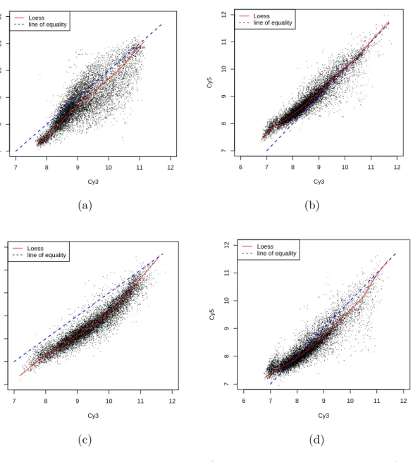
3.1 The design details of the skin cancer experiment. . . 70 3.2 Comparison of LOESS and the new method. In the scenario of the
example in the Figure 3.8, the new method has smaller amount of the sum of the squares of the difference between the normalized reconstructed data and original data than LOESS in both of the Cy3 and Cy5 channels. . . 102
4.2 Comparison of numbers of rejected genes by using different error rates in the leukaemia experiment. . . 123 4.3 Hedenfalk’s breast cancer data: the estimation of π0 using three
different mixture models. . . 156 4.4 The Callow’s lipid metabolism data: the estimation of π0 using
three different mixture models. . . 162 4.5 The estimation ofπ0by our method (using model of beta mixtures)
and Storey’s QVALUE for the 16 simulated data. . . 166
2.1 The four main effects result in six two-factor interactions (TG, TD, TA, GD, GA, DA). . . 10 2.2 Diagrammatic representations of the designs of six microarray
ex-periments. Each microarray array is represented by an arrow. The head of the arrow indicates that the sample was labeled with Cy5, while the tail represents a sample that was labeled with Cy3. . . . 16 2.3 Two microarray experimental design with the same layout (3
treat-ments and 6 arrays) but different allocation of sample replicates. . 27 2.4 The L-optimal designs of microarray experiment for 3 treatments
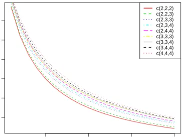
and 6 arrays with respect to different combinations of numbers of independent biological replicates for each treatment. . . 35 2.5 Comparisons of the reciprocals of L-optimality scores for the 9
designs shown in Figure 2.4 across the range of ρ from 0 to 4. . . 36 2.6 A cDNA microarray L-optimal design with 5 treatments and 15
arrays. The first treatment has only two independent biological replicates available while the rest of treatments have six indepen-dent biological replicates. . . 38 2.7 Comparisons across the dye-swap design and the alternative design
under L-optimality and D-optimality criteria. . . 39
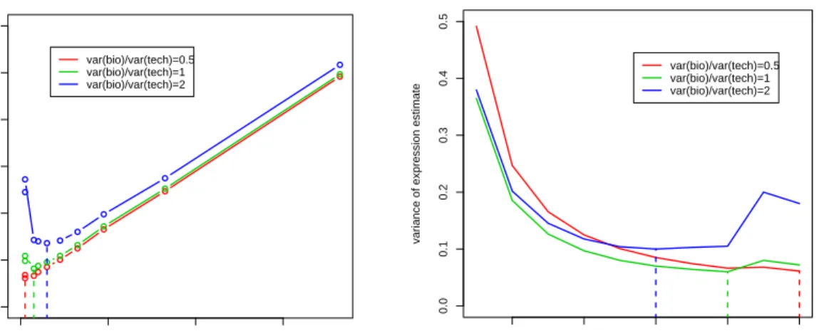
2.10 An example of optimal pooling by minimizing the estimation vari-ance V(¯x) = σ²2
nsna +
σ2
η
na, subject to not overrunning one’s budget
B =nsnaCs+naCa. . . 56
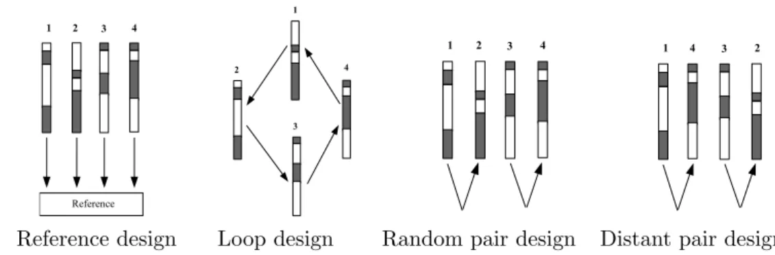
2.11 Illustration of four alternative experimental designs (Fu and Jansen, 2005). . . 58
3.1 The log-transformed data (after taking global normalization) from four different cDNA slides from the skin cancer experiment. . . . 72 3.2 Dye normalization for the second skin cancer array. . . 79 3.3 The two dye response models for a pixel in a spot on a dual-channel
microarray. . . 82 3.4 Dye effect patterns are caused by the dissimilarity of the two dye
response curves (see Equation (3.8)). . . 86 3.5 An example of the pixel level and spot level relationship for simple
dye response model. . . 87 3.6 A spot’s nonlinear dye response is generated by taking the average
of its pixels’ linear dye responses. . . 91 3.7 The difference between the Cy3 dye response function (the cdf of
normal distribution with mean 8 and variance 1) and the Cy5 dye response function (the cdf of normal distribution with different combinations of mean and variance value) results in a variety of dye effect patterns. . . 99
mean and variance of Cy3 dye response function is fixed to be 8 and 1, and the standard deviation of variation,σε, is set to be 0.1. 101
3.9 An example of comparison of the performance of the new method and LOESS method. The input Cy3 and Cy5 gene expression data (with dye effect) is simulated from the example shown in Figure 3.8. . . 104 3.10 Comparison of the performance of the new method and LOESS
method for a variety of scenarios. . . 106 3.11 An example of dye effect normalization using real skin microarray
gene expression data from experiment. . . 107
4.1 Analysis of Hedenfalk’s breast cancer data using the beta mixture distributions. . . 157 4.2 Analysis of Hedenfalk’s breast cancer data using the one-parameter
uniform mixture distributions. . . 158 4.3 Analysis of Hedenfalk’s breast cancer data using the uniform
mix-ture distributions. . . 159 4.4 Analysis of Callow’s lipid metabolism data using the beta mixture
distributions. . . 163 4.5 The histograms of p-values for 16 simulated datasets. The title
of each subfigure indicates the two parameters π0 and δ used for
generating the dataset. . . 167 4.6 Analysis of the Hedenfalk’s breast cancer data using the model of
beta mixtures. . . 168
4.8 The lFDR estimates by our method (using model of beta mixtures) and Liao’s method for 16 simulated datasets in Section 4.6.4. . . . 170 4.9 The pFDR estimates by our method (using model of beta
mix-tures) and Storey’s QVALUE for 16 simulated datasets in Section 4.6.4. . . 171
A.1 Directed graphs describe six typical situations involved in comput-ing the covariance of gene expressions of the ith and jth microar-rays. . . 184
Introduction
Since worldwide efforts to sequence genomes began formally in 1990, rapid tech-nological advances have been introduced so that over the past few years a large number of organisms have had their genomes completely sequenced, including yeast, worm, fly, mouse and human. But the billions of bases of DNA sequence do not tell us what all the genes do and how sets of genes interact with each other in the genome. In order to solve these problems, a lot of efforts are being made to the functional genomics which is an area of genome research concerned with assigning biological function to DNA sequences. For functional genomics new technologies are being applied to take full advantage of the large and rapidly increasing body of sequence information. Among the most powerful and ver-satile tools are DNA microarrays, which allow simultaneous monitoring of the expression levels of numerous genes.
The principle of a microarray experiment, as opposed to the classical northern-blotting analysis, is that mRNA from a given cell line or tissue is used to generate a labelled sample (sometimes termed the target), which is hybridized in parallel to a large number of DNA sequences (sometimes termed the probes), immobilized
on a solid surface in an ordered array. Tens of thousands of transcript species can be detected and quantified at the same time. Although many different mi-croarray systems have been developed, the most commonly used systems today can be divided into two groups, according to the arrayed material: complemen-tary DNA (cDNA) and oligonucleotide microarrays. High-density oligonucleotide microarray experiments provide direct information about the expression levels in a mRNA sample of the 200,000-500,000 probed DNA sequences. By contrast, cDNA microrarray experiments typically involve hybridizing two mRNA sam-ples, each of which has been converted into cDNA and labelled with its own fluorophore (Cy3 and Cy5 dyes) respectively, on a single glass slide that has been spotted with as many as 10,000-20,000 cDNA probes. Data from such experi-ments provide information on the relative expression of the sample genes, which correspond to the probes.
Microarray experiments usually generate large and complex multivariate data sets, and some of the greatest challenges lie not in generating these data but in the development of statistics tools to design the experiment and analyse the large amount of data. In this thesis, our interest is the cDNA microarray and we try to discuss three different topics in the statistical analysis of the cDNA microarray experiments in Chapter 2, 3 and 4 respectively.
The first general topic is relevant to the optimal design of cDNA microarray experiments. As two samples can be applied or “hybridized” to a single cDNA microarray, the array is a blocking factor. Another nuisance factor is the two-level dye factor, as the gene expressions in the two samples on an array are measured via a Cy3 and a Cy5 dye. When more than two sample conditions or treatments are of interest, then not every sample can appear on an array so that some form of an incomplete-block design should be considered. This brings with it a challenge
how to design the experiments (i.e. which samples should be co-hybridized on a single array) so that the efficiency and reliability of the microarray data can be improved and the precise estimates of biologically important parameters can be obtained.
Many of the microarray designs currently used are the so-called reference designs. In this type of design, each sample condition of interest is compared with a fixed, standardized condition. Making all comparisons to a reference sample is however inefficient, because half of the hybridization resources are allocated to the reference sample, which is usually of little or no interest. Alternatives to reference designs have been suggested. Dye swap designs and loop designs have gained some popularity. However, Kerr and Churchill (2001a) have pointed out that dye swap designs are quite inefficient and loop designs are optimal only for a relatively small number of conditions. Wit et al. (2005) have shown how the application of a simple optimization algorithm, simulated annealing with local design moves, to incomplete-block designs with block size 2 can find optimal or near-optimal designs for given number of conditions and arrays based on different optimality criterion. However, this optimization strategy just assumes that for each sample condition (treatment) the number of independent biological replicates is not less than the total number of replicates needed. Unfortunately, in some cases this assumption does not stand (i.e. no enough biological replicates available) so that technical replicates have to be used. Then a question arises: How to assign the biological and technical replicates to the arrays in an optimal way? To deal with this problem, we follow the spirit of the simulated annealing framework for optimal design and develop a modified optimization strategy to find the optimal or near-optimal design and allocation of biological and technical replicates in the first part of Chapter 2.
In recent years more and more biologists begin to consider multi-factorial microarray experimental set-ups to identify differentially expressed genes, e.g. Caetano et al. (2004). The problem of how to find optimal (efficient) factorial design has received some attention. For example, Glonek and Solomon (2004) used A-optimality to find optimal designs of factorial experiment with a small number of factors. In the second part of Chapter 2, we use a new multi-factorial design optimality criterion called Q-optimality (Tsai et al., 2000) and show that under the simulated annealing framework it can be used to search near-optimal multi-factorial microarray experimental designs.
Statistical design of microarray aims at reducing unwanted variations to in-crease the precision of the quantities of interest. Pooling true biological RNA replicates is a cost-effective way to achieve this goal. In the third part of Chapter 2, we make some practical suggestions about optimal pooling samples for a mi-croarray experiment. We find a replication scheme that minimizes the variance of the experiment under the constraint of fixing the total cost at a certain level. Recently the combined study of gene expression and molecular marker data has been proposed as a novel strategy for the analysis of regulatory networks. Costs of such studies are high and require that resources microarrays and samples are used as efficiently as possible. Fu and Jansen (2005) propose a new design called distant pair design for this kind of studies, which co-hybridizes sample individuals with dissimilar genomes. The corresponding optimality criterion is defined for the case of single marker and is further extended to the case of multiple markers by simply averaging the criterion for single marker. We believe the extension is not very proper and propose a new criterion for the case of multiple markers as an alternative in the final part of Chapter 2.
technology of cDNA microarray is based on measuring optical intensities of dye labeled cDNA that has hybridized to gene-specific probes on the microarray. Two different types of dyes Cy3 and Cy5 are commonly used for the two samples on the array. Ideally, these two dyes should have the same properties so that the direct comparison between the two gene expression data of the two channels can be meaningful. However, the fact is that the dyes have slightly different properties and the relative efficiency of the dyes usually vary across the intensity range in a “banana-shape” way. In order to remove the dye effect as much as possible, several methods have been proposed, such as dye-swap normalization by Yang et al. (2002b) and intensity-dependent dye normalization (LOESS) by Yang and Speed (2003). In Chapter 3 we suggest a new dye effect normalization method based on modeling dye response functions and dye effect curve. The performance of our method is compared to LOESS by using simulated microarray gene expression data and real microarray data.
In a typical cDNA microarray experiment, a large number of gene expressions are usually measured. When these variables are simultaneously screened by a statistical test, it is necessary to consider the adjustment for multiple hypothesis testing. Quite a few error rates of multiple testing such as false discovery rate (FDR), positive false discovery rate (pFDR) and local false discovery rate (lFDR) have been proposed and widely used to address this issue. A related problem is the estimation of the proportion of true null hypotheses, π0. In Chapter 4, we
first review the background of multiple hypothesis testing and its error rates, then we deal with the estimation ofπ0 by modeling p-values from the experiment with
finite mixtures with unknown number of components. Three different mixture models are considered. A newly developed MCMC method, allocation sampler (Nobile and Fearnside, 2007) is not only applied to estimate π0 but also pFDR
and lFDR for both real and simulated microarray gene expression data.
Since this thesis deals with three very different topics in the statistical anal-ysis of cDNA microarray experiments in Chapter 2, 3 and 4, we include a more detailed introduction section for each of these chapters.
The Chapter 5 is a conclusion of the whole thesis and discussion of further potential research opportunities.
Optimal design of cDNA
microarray experiments
2.1
Introduction to cDNA microarray
experi-mental design
Spotted complementary DNA (cDNA) microarray is a powerful and cost-effective technology which provides molecular biologists and geneticists with a tool to monitor thousands of genes simultaneously (Brown and Botstein, 1999). Since its introduction in 1995 (Schena et al., 1995), this revolutionary technology has greatly influenced and accelerated the molecular biological and medical research. A cDNA microarray, also called two-channel microarray or spotted microar-ray, typically consists of thousands of microscopic spots of DNA oligonucleotides (gene). For each spot, it measures the relative abundance of the DNA samples (under two different treatments) hybridized to the spot. The experiment usually consists of several steps. First, pools of mRNA derived from experimental or
clinical samples under two treatments are reversed-transcribed into cDNA and labelled with Cy3 (green) and Cy5 (red) fluorescent dyes respectively. Second, the two labelled cDNA pools are mixed in equal proportions and hybridized to the probes on a solid surface (i.e. array), which can be glass or a silicon chip. The probes are synthesized prior to being spotted onto the array surface and can be oligonucleotides, cDNA or small fragments of PCR products that corre-spond to mRNAs. Third, probe-target hybridization occurs on the array: the probe catches the complementary matched cDNA and the unhybridized cDNA is washed away. Finally, the red and green signal intensities are separately read out for each spot on the array by a laser scanner. The ratio of the optical signal intensities represents the relative abundance of the corresponding mRNA under two treatments. A higher intensity of one treatment over the other means that the spot (gene) is more “active” under the former.
2.1.1
Microarray experimental effects
The primary objective of a microarray experiment is to look for changes in gene expression across factors of interest. The factor could be the different type of samples (tissues) or the different drug or stress treatments (conditions) or the different stages of a biological process (time points).
Basically, there are four microarray experimental effects:
1. Treatments (T): the categories of the factor of interest.
2. Genes (G): spotted sequences (e.g. genes, ESTs, or DNAs).
3. Dyes (D): Cy5 (red) and Cy3 (green) labels.
Therefore there are 15 experimental effects in a microarray experiment in total, including four main effects (T, G, D, A), six two-factor interactions (TG, TD, TA, GD, GA, DA), four three-factor interactions (TGD, TGA, TDA, GDA) and one four-factor interactions (TGDA).
Treatment main effects (T) account for overall differences in treatments. Such differences could arise if some treatments have more transcription activity in general.
Gene main effects (G) occur when certain genes emit a higher or lower fluo-rescent signal overall, compared to other genes. These effects arise because some genes have generally higher or lower levels of expression than others irrespective of treatments, dyes or arrays.
Dye main effects (D) measure the difference in the two dye fluorescent labels. For example, one dye may be consistently brighter than the other when averaged over the other factors.
Array main effects (A) account for differences between arrays, averaged over all genes, dyes, and treatments. These effects arise if, for example, arrays are probed under inconsistent conditions that increase or reduce hybridization effi-ciencies of the labeled cDNA.
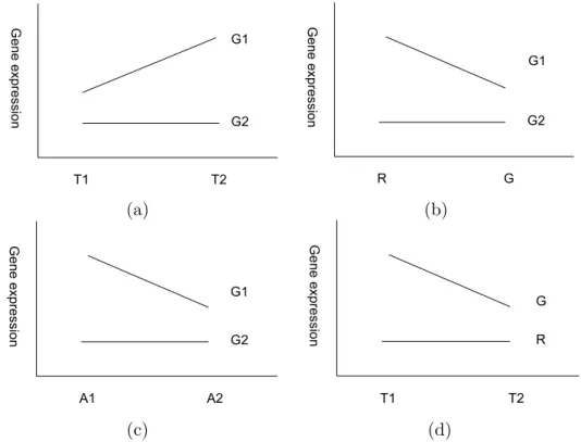
Treatment × Gene (TG) interactions arise when the relative expressions of specific genes are different from one treatment to the other (when averaged over arrays and dyes). This can be illustrated graphically in Figure 2.1 (a). These effects are the most important in the experiment and their identification and quantification is often the main objective of the experiment.
Dye × Gene (DG) interaction effects occur when differences in intensity be-tween Red and Green dyes are different from one gene to the other. This can be illustrated graphically in Figure 2.1 (b). This can happen when cDNA sequences,
(a) (b)
(c) (d)
Figure 2.1: The four main effects result in six two-factor interactions ( TG,
TD, TA, GD, GA, DA). Here we illustrate the four most impor-tant interactions effects, which are (a) gene-treatment interac-tion, (b) gene-dye interacinterac-tion, (c) gene-array interaction and (d)
dye-treatment interaction.
matching specific genes on the chip, incorporate red dye molecules at a different rate than green molecules while sequences specific to other genes show the reverse trend. This effect is quite likely due to the chemistry of dye incorporation and so must be accounted for in any array experiment. Note that if this effect exists and has not been detected, estimates of relative expressions are biased and may lead to misleading results.
Array×Gene (AG) interaction effects or spot effects may arise because there is no complete control over the amount and concentration of cDNA immobilized from one array to the next. This can be illustrated graphically in Figure 2.1 (c). A Dye×Treatment (DT) interaction effect for given gene A is shown in Figure
2.1 (d). It may occur in the experiment when one fluorescent dye hybridizes more with cDNA from treatment T1 than from T2, but the other dye is consistent. If this sort of effect was consistent over many genes and arrays, we should find a DT interaction. However, we do not always see this happen in practice.
Besides the above four main effects and four two-factor interaction effects, it is difficult to relate the other remaining 7 higher-order interaction effects to the microarray experimental process. For example, two-factor interaction effects like Array×Dye (AD), Array×Treatment (AT), and three- factor interaction effect like Array × Dye× Treatment (ADT) do not involve the genes. It is difficult to relate any of these to the process underlying microarrays and to suppose a reason why such interactions would come into play. Array×Dye×Gene (ADG), Array × Treatment × Gene (ATG), Dye × Treatment × Gene (ATG), and Array × Dye×Treatment×Gene (ADTG) effects all do involve the genes. The presence of such interactions would mean there is gene-specific variation attributable to a particular array and dye, a particular array and treatment, a particular dye and treatment, or a particular array, dye, and treatment combination. Again, these high-order interactions are difficult to relate to the physical and chemical processes that make up this technology and so they are generally assumed not to occur. This assumption should, however, be checked in practice.
2.1.2
Replication
In noisy experiments, replication is an important concept. It is necessary in order to reduce the variability inherent in microarray experiments. Generally, there are two types of replication: technical and biological. One form of technical repli-cation is spot duplirepli-cation. If space permits, cDNAs can be spotted in duplicate
on every array and the degree of conformity between duplicate spot intensities is a good indicator of the quality of the slide and hybridization. It is advisable, however, that duplicate spots be well spaced apart rather than spotted adjacently as this facilitates inspection of the degree of variability across the slide. Another type of technical replication is the array replicate. It is the replication of multi-ple arrays hybridized with RNA from the same sammulti-ple (preparation). Due to the length and complexity of a microarray experiment, it is crucial to check that the results were not obtained by mere chance fluctuations, but rather arise from gen-uine underlying biological variation. Technical replication can be used to obtain an average measurement from each sample or to quantify systemic variation.
Biological replicates could be hybridizations performed using RNA from in-dependent preparations from the same source, or preparations from biologically distinct sources, such as different organisms or different versions of a cell line. The latter type of biological replication is more popular since it encompasses greater variation in measurements. For instance, an experiment investigating drug treatment in mice is subject to the variation within the mice population, such as differences in immune system, sex, and age. The greater variability in-herent in this form of replication contributes to a broader generalization of the experimental results.
In conclusion, a researcher should use biological replicates to validate gener-alizations of conclusions and technical replicates to estimate and eliminate the variability associated with the hybridization.
2.1.3
Pooling
Due to the instability of RNA, it can be difficult to extract sufficient material for hybridization, especially if the sample is to be spread over several replicates. Sometimes the RNA required for even a single array may be unachievable for small organisms. In such circumstances, the RNA from several samples could be pooled by biologists to make up the volume needed, but this practical constraint may alter the objectives of the investigation. After pooling the researcher is no longer able to make inferences about the individual samples, but only about the population from which they were drawn. This restriction may not be too important when the purpose of analyzing individual samples is to make inference on the population, which is typically the case.
When one wishes to characterize a population, pooling might reduce the over-all costs of an experiment because arrays are often, though not always, more expensive than the generation of the samples. The cost of an experiment can be substantially reduced by measuring a number of pooled samples on a smaller number of arrays. Pooling multiple replicates will have the effect of decreas-ing the population variance and diminishdecreas-ing random fluctuations. However, the researchers should be aware of situations where it is not appropriate to pool sam-ples. For example, when studying the effect of a drug on cancer patients, the gene expression in specific patients is of interest. In this case, hybridizations with individual samples should be carried out. On the other hand, in an inves-tigation of two inbred homozygous ecotypes of Arabidopsis, differences between the individual plants are not of interest, so pooling may be justified.
2.1.4
Experimental designs
A single microarray experiment is just a comparison between two RNA samples collected under different treatments, both are applied to the same dual-channel array. The array can be considered as a blocking factor, similar to a plot of land in an agricultural field trial. Therefore, basic microarray experimental design is a block design with block size two. Since design can involve direct or indirect comparisons, there are usually more than one way to pair and label samples for cDNA microarrays.
2.1.4.1 Direct comparisons
Due to the parallel nature of dual-hybridization microarrays, the most efficient design to compare two samples is to directly compare them on the same array. By pairing samples, we can examine the relative abundance of the two samples, while accounting for variation in spot size that would otherwise contribute to the error.
Dye swap is a simple and effective design for the direct comparison of two samples. This design compares two samples by using two arrays instead of one. On array one, one sample is assigned to the red dye, and the other sample is assigned to the green dye. On array two, the dye assignments are reversed. See Figure 2.2 (a). In the vocabulary of experimental design, a dye-swap design is a complete block design, taking the form of a 2×2 Latin Square (Table 2.1). This simple design plan removes dye effect from the measurements by taking the mean log expression ratio on each probes for both dye-swaps. This arrangement can also be repeated by using an even number of arrays (e.g. four or six or more) to compare the same two biological samples. See a simple example in Figure 2.2
Red dye (Cy5) Green dye (Cy3) Array 1 Sample 1 Sample 2 Array 2 Sample 2 Sample 1
Table 2.1: A Latin Square design to compare two samples directly.
(b). Repeated dye-swap experiments are used for reducing technical variation (although not very popular in practice). If independent biological samples are used, the experiment will account for both technical and biological variation.
If a microarray experiment involves more than two samples under different treatments, then not every sample can appear on every array and some form of incomplete block design should be considered instead. This brings with it a challenge of how to design the experiments (i.e. which samples should be co-hybridized on a single array) so that the efficiency and reliability of the microarray data can be improved and precise estimates of biologically important parameters can be obtained.
(a) (b)
(c) (d)
(e) (f)
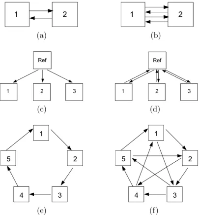
Figure 2.2: Diagrammatic representations of the designs of six microarray
experiments. Each microarray array is represented by an arrow. The head of the arrow indicates that the sample was labeled with Cy5, while the tail represents a sample that was labeled with Cy3. (a) Direct comparison (dye-swap) between two samples; (b) A repeated dye-swap experiment between two samples with four arrays; (c) A reference design (indirect comparison) studies three samples; (d) A variation of the reference design (Figure 2.2 (c)) using a dye swap for each comparison; (e) A loop design with five treatments; (f) An interwoven loop design for five treatments
2.1.4.2 Reference design
The reference design of Kerr and Churchill (2001a) affords a means of indirect comparison, and is commonly used for studying multiple treatments of a factor of interest. It is called a reference design because it uses an aliquot of a common reference RNA as one of the samples hybridized to each array (See a simple example in Figure 2.2 (c)). This is done so that the intensity of hybridization to a spot for a test sample is measured relative to the intensity of hybridization to the same spot on the same array for the reference sample (typically of no scientific interest).
The reference sample is usually labelled with one dye and acts as an inter-mediate and allows an indirect comparison between the samples of interest, all of which are labelled with the other dye. This means that treatment effects are completely confounded with dye effects. Consequently, the effects of interest, treatment×gene (TG) are completely confounded with dye× gene (DG) effect. If the dye×gene (DG) effect is significantly noticeable, then the microarray data from reference designs have to be validated before making conclusions. Alterna-tively a reverse-dye comparison could be incorporated in a biological replicate to account for the dye effect on specific genes (i.e. use two arrays in a dye-swap configuration, see an example in Figure 2.2 (d)). Another disadvantage is that making all comparisons to a reference sample can be inefficient, because half of the hybridization resources (e.g. arrays) are allocated to the reference sample, which is presumably of little or no interest.
In spite of its inefficiency, the reference designs are very popular among practi-tioners. There are several reasons. First of all, reference designs are very intuitive to understand: by being measured against the same reference the values across different arrays can be directly compared with one another. Secondly, it is also
very straightforward to use the same reference to control variation in each spot and there are only two path-steps connecting two samples in a reference design, so each comparison can be made with equal efficiency. Thirdly, as long as the amount of reference sample is not limiting, the reference design can be extended to handle a large number of treatment levels. From a practical perspective, every new sample in a reference experiment is handled in the same way. This reduces the possibility of laboratory error and increases the efficiency of sample handling in large projects. Finally, the reference design is robust to loss of arrays resulting from poor quality hybridization, although the loss of one array may entail the complete loss of information about one nonreference sample.
2.1.4.3 Loop design
The loop design is an alternative to the reference design (Kerr and Churchill, 2001a). Loop designs compare two treatments via a chain of other treatments without the need for a reference treatment. The nominal last treatment is con-nected with the nominal first treatment. A simple loop design with five treat-ments is shown in Figure 2.2 (e).
The loop design is more efficient than the reference design since the former can measure twice the number of replicates by using the same number of arrays as the latter. In simple loop designs, treatments are balanced with respect to dyes because each sample is labeled once with the red dye and once with green dye. This balance means that dye effects are unconfounded with treatment effects, so treatment × gene effects are unconfounded with dye × gene effects. Thus the effects of interest will not be biased by any strange behavior of genes with respect to dyes.
First of all, contrasting two treatments far apart in the loop involves modeling many indirect effects, corresponding to the arrays linking the two treatments of interest. This adds substantial variance to many of these contrasts (Khanin and Wit, 2004). Thus loop designs are not ideal for large numbers of treatment levels (Kerr and Churchill, 2001a). Secondly, loop designs are less robust against the presence of bad quality arrays: two or more bad arrays can break the loop apart and collapse the experiment. However, this problem can be solved by repeating the bad quality arrays. Finally, adding additional treatment levels to the loop design is not as easy as in the reference design.
2.1.4.4 Interwoven loop design
As alternatives to the reference design, loop designs have gained some popularity among practitioners. However, Kerr and Churchill (2001a) have pointed out that loop designs are optimal only for a relatively small number of treatments. Wit et al. (2005) identified a type of designs, interwoven loop designs, that seems to have good optimality properties.
The interwoven loop design, sometimes also called the replicated loop design, is an extension of the original loop design (Churchill, 2002). If the number of microarrays is a multiple k of the number of treatments p, then an interwoven loop designIp(1, j2, ..., jk) can be defined as an ordinary loop design (withk
repli-cates) where each sample is also measured with respect to the samples that are
j2, j3, . . . , jk jumps further along the circle. An interwoven loop design example
I5(1,2) is shown in Figure 2.2 (f). When the number of treatments is quite large,
interwoven loop designs have been demonstrated to have very nice properties: easy to implement, high efficiency, automatic dye balance (Wit et al., 2005).
2.1.4.5 Alternative designs
Besides the designs discussed above, it is possible to find other good designs. John and Mitchell (1977) suggested exhaustive search algorithms for finding the optimal design within particular classes of designs, but these have only limited practical applicability. John and Williams (1995) discussed the employment of simulated annealing for optimal row-column designs that could be directly ap-plicable to dual channel microarray designs. Kerr and Churchill (2001b) used a computer program for graphs and taking into account other design properties such as balance, they searched exhaustively for non-isomorphic connected de-signs. However, this is only possible when the number of microarrays is small, typically less than 10.
Inspired by these works, Wit et al. (2005) applied a simple optimization strat-egy, also based on simulated annealing, to obtain optimal or near optimal mi-croarray experimental designs in the sense of minimizing a criterion based on the variance of all the possible contrasts between treatments.
2.2
Optimal design with biological and
techni-cal replicates
Wit et al. (2005) applied an optimization strategy based on simulated annealing to search for near-optimal designs for any number of treatments and any num-ber of arrays. However, the optimization strategy simply assumes that for each sample condition (treatment) the number of biological replicates available should exceed the number of arrays it involves. In other words, there should be enough independent biological samples for each treatment. Unfortunately, this is not always possible. For example, sometimes biological material may be very lim-ited when one is conducting research on mammals (Byrne et al., 2005). In that case, one has to use technical replicates instead of biological replicates. Then we have the following problem: How to assign optimally the biological and technical replicates to the arrays?
In this section, we develop a modified optimization strategy using simulated annealing to find near optimal designs and near optimal allocations of biological and technical replicates.
2.2.1
A statistical model for microarray gene expression
intensity
A cDNA microarray experiment contains information about the expression of thousands of genes. Each spot on the array measures two gene expression signals under two treatments associated with two dyes Cy3 and Cy5. Since the signals are essentially positive and typically behave multiplicatively, rather than additively, the logarithmic transformation can be applied to transform the optical intensity
of a spot associated with a particular gene from the multiplicative scale into an additive scale (Chen et al., 1997). Here, we model the gene expression intensity for each channel separately. This allows us to compute the variance of any contrast, and to determine the effect of biological and technical replication on the variance. Consider the gene expression models for the two channels c1 and c2 of an
array:
logxc1k1r1 =θc1 +S+D+²c1k1 +ηc1k1r1, (2.1) logxc2k2r2 =θc2 +S+D+²c2k2 +ηc2k2r2, (2.2) where xckr is the signal intensity, θc is proportional to the true gene expression
under channel c, S is the nuisance effects such as spot effect and spatial effect,
D is the dye effect. Note that we set the spot and spatial effect D be the same for the two channels for the reason that they are assumed to affect each of the channels similarly because the two channels has the same spot size and have the same position-dependent sources of variation. Dye effectDis also assumed to be the same for the two channels for the purpose of simplicity.
²ck is the biological variation for individual k under channel c and assumed
to be normal distributed with mean zero and variance σ2
b, ηckr is the technical
variation for therth replicate of the individualk under channelcand assumed to be normal distributed with mean zero and variance σ2
t. We make several further
assumptions for biological variation and technical variation.
• ² and η are independent from each other no matter what the subscript.
• When c1 =c2 and k1 =k2, Cov(²c1k1, ²c2k2) =σ
2
b; otherwise,
Cov(²c1k1, ²c2k2) = 0.
• When c1 =c2, k1 =k2 and r1 =r2, Cov(ηc1k1r1, ηc2k2r2) =σ
2
otherwise, Cov(ηc1k1r1, ηc2k2r2) = 0.
The difference between the gene log expressions of the two treatments in one spot is equal to the log-ratio of the gene expressions. For a particular gene on an array, we can calculate the log-ratio of the gene expressions of the two treatments:
yc1c2k1k2r1r2 = logxc1k1r1 −logxc2k2r2
= θc1 −θc2 +²c1k1 −²c2k2 +ηc1k1r1 −ηc2k2r2, (2.3)
2.2.2
Parametrization and estimation
In a comparative microarray experiment across p treatments, the parameters of interest are: θ = (θc1, θc2, . . . , θcp)
T, where θ
ci is the average log gene expression
for channelci. The log-ratio formulation of the microarray gene expression model
is informative about the gene expression θ only up to an additive constant. In order to identify the parameter θ, we should impose some constraint such as setting the sum of θ to zero or setting the first element of θ to be zero, i.e.
θc1 = 0.
Instead of the vector of absolute expressionθ, we can reparameterize the model with a vector of δ∗ = {δ
cicj|ci > cj}, where δcicj = θci −θcj. This
parametriza-tion contains all the possible relative (differential) expressions, but it is over-parameterized. Therefore we use a canonical parametrization δ consisting of
p−1 terms, δ = (δc2c1, . . . , δcpc1)
T. Any other item in δ∗ can be regarded as a
of the gene expressions of two treatments ci and cj of an array as follows,
ycicjkikjrirj = δcicj +²ciki −²cjkj+ηc1k1r1 −ηc2k2r2
= δcic1 −δcjc1 +²ciki −²cjkj+ηc1k1r1 −ηc2k2r2. (2.4)
Assuming that the microarray experiment involves narrays (i.e. 2n channels) and p treatments, we can write the log-ratio gene expression intensity according to the spirit of Equation (2.4) for all the arrays respectively and then we have a system of n equations which can be described in matrix notation as follows,
y =Xδ+
p
X
i=1
Zi²i+η, (2.5)
where y is a n×1 vector of observations, X is an×(p−1) design matrix, δ is the (p−1)×1 canonical parametrization, Zi is a n×mi random effect matrix
for treatment i, ²i is a mi×1 vector of biological variation for treatment i and
is assumed to be normally distributed with zero-mean and covariance matrix
σ2
bImi, mi is the total number of independent biological replications available
under treatment i, η is a n×1 vector of technical variation and is assumed to be normally distributed with zero-mean and covariance matrix 2σ2
tIn. Here Imi
denotes the mi×mi identity matrix and In denotes then×n identity matrix.
If we let ε=Ppi=1Zi²i+η, then Equation (2.5) can be rewritten as
y=Xδ+ε, (2.6)
matrix Σ, which can be calculated from Equation (2.5) as Σ = p X i=1 σ2 bZiZit+ 2σt2In. (2.7)
If the elements of ε are uncorrelated with each other, Σ is a multiple of identity matrix. If not, then Σ can be found according to the experiment design. An example of computing Σ is discussed in the next subsection.
By using maximum likelihood estimation (MLE), we get a generalized least squares (GLS) estimator,
ˆ
δ = (XtΣ−1X)−1XtΣ−1y, (2.8)
which is the best linear unbiased estimator (BLUE) for δ, in the sense of having smallest sampling variability in the class of linear unbiased estimators, provided Σ is known (according to the Gauss-Markov Theorem). The variance of the estimator not only depends on the design matrix X but also on the covariance matrix Σ,
Var(ˆδ) = (XtΣ−1X)−1. (2.9)
2.2.3
An example: computation of
Σ
The computation of Σ is just the computation of the covariance of the expressions of any two arrays. Here we summarize the rules of computation in the following (see the details in Appendix A):
1. When the two arrays have one common treatment and have the same tech-nical replicate under that treatment, the covariance isσ2
b+2σt2(if the arrays
have the same type of dye attached on that treatment) or−σ2
arrays have different types of dye attached on that treatment).
2. When the two arrays have two common treatments and have the same technical replicates under both of the treatments, the covariance is 2σ2
b +
2σ2
t (if the arrays have the same types of dye attached on the treatments)
or −2σ2
b + 2σt2 (if the arrays have different types of dye attached on the
treatments).
3. When the two arrays have two common treatments and have the same technical replicate under one treatment, the covariance is σ2
b + 2σ2t (if the
arrays have the same type of dye attached on that treatment) or−σ2
b+ 2σt2
(if the arrays have different type of dye attached on that treatment).
4. Under other situations, the covariance is zero.
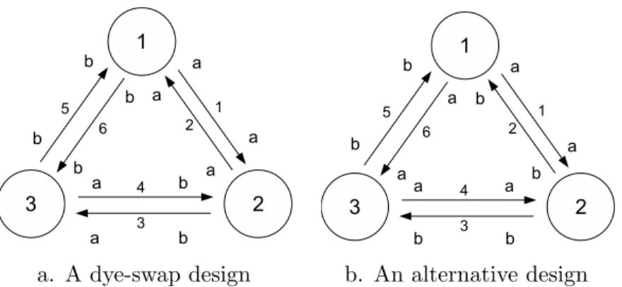
Following the above rules, we can get the explicit form of covariance matrix Σ according to the experiment layout. As an example, let’s consider an experiment with 3 treatments and 6 arrays. Each treatment has 2 biological (a and b) samples split into 2 technical replicates. Two design layouts of this experiment are shown in Figure 2.3, and two corresponding explicit forms of Σ are deduced in the following. For the dye-swap design in Figure 2.3 (a), we have
Σ = 2σb2 1 −1 0 0 0 0 −1 1 0 0 0 0 0 0 1 −1 0 0 0 0 −1 1 0 0 0 0 0 0 1 −1 0 0 0 0 −1 1 + 2σt2 1 0 0 0 0 0 0 1 0 0 0 0 0 0 1 0 0 0 0 0 0 1 0 0 0 0 0 0 1 0 0 0 0 0 0 1 ,
a. A dye-swap design b. An alternative design
Figure 2.3: Two microarray experimental design with the same layout (3
treatments and 6 arrays) but different allocation of sample repli-cates.
For the alternative design in Figure 2.3 (b), we have
Σ = 2σ2 b 1 0 0 1 2 0 1 2 0 1 1 2 0 1 2 0 0 1 2 1 0 − 1 2 0 1 2 0 0 1 0 − 1 2 0 1 2 − 1 2 0 1 0 1 2 0 0 − 1 2 0 1 + 2σ2 t 1 0 0 0 0 0 0 1 0 0 0 0 0 0 1 0 0 0 0 0 0 1 0 0 0 0 0 0 1 0 0 0 0 0 0 1 .
Although both designs have the same design matrix, the different allocation of biological and technical replicates makes these designs have very different Σ. The non-zero entries off the diagonal in the covariance matrix reflects that some arrays (gene expressions) are correlated with each other due to having common biological replicates.
Note that when there are enough independent biological replicates available (e.g. 4 biological replicates for each treatment), we would have a very simple Σ:
Σ = 2σ2 b 1 0 0 0 0 0 0 1 0 0 0 0 0 0 1 0 0 0 0 0 0 1 0 0 0 0 0 0 1 0 0 0 0 0 0 1 +σ2 t 1 0 0 0 0 0 0 1 0 0 0 0 0 0 1 0 0 0 0 0 0 1 0 0 0 0 0 0 1 0 0 0 0 0 0 1 .
In this special situation, the variance of the estimate ˆδcan be simplified to be Var(ˆδ) = (XtX)−1σ2, where σ2 = 2σ2
b + 2σt2, which is exactly the case discussed
in Wit et al. (2005).
In the same way, for any microarray experimental design, we can compute Σ and decompose it into two separate parts: a biological part and a technical part.
Σ = 2σ2
bΣB+ 2σ2tΣT,
where ΣT is always an identity matrix and ΣB can be easily computed given the
details of the biological and technical replicates allocation. We can also rewrite Equation (2.10) as:
Σ = 2σt2(ρΣB+I).
where ρ = σb2
σ2
t and ρ is assumed to be a constant and we should know its value
before planning the experimental design. In practice, ρ can not be known before experiment because it can only be estimated from the result of the experiment. As a way out, for each gene (spot)ρ could be estimated from previous experimental
data by using restricted maximum likelihood (REML) or maximum likelihood (ML), but these methods are very inaccurate with the small sample sizes often used in microarray studies. In recent approaches, using all the spots on the array has been suggested to improve estimation. For example, Smyth, Michaud and Scott (2005) use empirical Bayes estimation to improve the estimate of σ2
t and
assume a singleρvalue that can be computed from all the genes. Cui et al. (2005) use shrinkage estimation to improve the estimation of all the variance components and so on. In this section, we do not concern ourself with the estimation of ρ(σ2
t
and σ2
b) and assumeρ is already known.
2.2.4
Optimality criteria
Optimal design is a matter of applying the observations to the treatments in such a way that the parameters of interest are estimated most “optimally”. For microarray experiments, there is a limited number of arrays available as well as a certain amount of RNA from several biological treatments of interest. The ques-tion then is which samples should we put on which arrays in order to maximize the precision of resulting parameter estimates?
The definition of precision depends on what optimality criterion is used. There are are several quite popular forms of design optimality, such as D-optimality, A-optimality and its related L-A-optimality (Wit et al., 2005). The covariance matrix of the parameter estimates plays a key role in all of these three forms of design optimality.
D-optimal design seeks to minimize the determinant of the covariance matrix of the parameter estimates. A-optimal design is the design for which the average variance of the parameter estimates is minimal. L-optimal design is a modified A-optimal design which minimizes the average variance of the estimates of several
linear functions of the parameters.
The appropriate criterion for comparing designs for a specific experiment should be closely related to the objectives of that experiment. If the aim is to acquire maximal precision of all differential gene expressions, it is better to use the canonical parametrization and choose L-optimality rather than A-optimality, because A-optimality depends on the particular parametrization that is chosen while L-optimality’s linear functions can map the canonical parameters into all possible contrasts between the treatments. If the aim is to minimize the gener-alized variance of all differential gene expressions, D-optimality is a choice which does not depend on the parametrization of the model.
In the next section we use simulated annealing to search for optimal or near-optimal designs, which not only consider the near-optimality of the design matrix, but also take into account the allocation of independent biological and technical replicates.
2.2.5
Simulated annealing implementation for finding
near-optimal designs
We denote the class of possible designs fornarrays,ptreatments and (s1, . . . , sp)
biological replicates with respect to parametrizationβ asχ(n, p, s, β), where s=
(s1, . . . , sp) the number of biological replicates available for treatments 1, . . . , p.
One way to select the optimal design consists in using discrete optimization over the space of design matrices χ(n, p, s, β). Since the design space is large, exhaustive searches are infeasible even for only moderately large n and p. We follow the simulated annealing framework in Wit et al. (2005) to find near optimal designs for arbitrary n,p, X and Z.
The simulated annealing algorithm to maximize an objective function f(x) works as follows. First of all, let (X, Z) be the current state, whereXis the design matrix and Z is the random effect matrix. Secondly, propose a new candidate state (X0, Z0), where X0 is the new design matrix and Z0 is the new random
effect matrix, from some proposal distribution q((X, Z) → (X0, Z0)). Then, the
candidate is accepted as the next state with probability:
min ( 1, µ f(X0, Z0) f(X, Z) ¶1/Ti q((X0, Z0)→(X, Z)) q((X, Z)→(X0, Z0)) ) , (2.10)
where Ti is the current temperature parameter that decreases with the iteration
index i. If the proposal p satisfies q(X0, Z0 → X, Z) =q(X, Z → X0, Z0) for all
(X, Z) and (X0, Z0), we have a simpler form of the acceptance probability:
min ( 1, µ f(X0, Z0) f(X, Z) ¶1/Ti) . (2.11)
If the candidate is rejected the next state is set to be the current state. The simulated annealing algorithm is started at a relatively high temperature T0, so
that at the beginning virtually all candidates are accepted. As the temperature is gradually decreased to zero, it becomes increasingly more difficult to accept moves to states that decrease f(X, Z). van Laarhoven and Aarts (1987) prove that under some conditions on the proposal distribution q (essentially irreducibility of the resulting Markov chain) and on the cooling schedule (Ti proportional to
1/log(i)) the simulated annealing algorithm converges with probability 1 to a global optimum.
In this paper, we choose exponential cooling schedules, such as Ti = T0ci
where c is a constant that is smaller than but close to 1. We use T0 = 10 and
c∈[0.99,1). The total number of iterations was set to achieve a preset low final temperature Tf inal = 0.0001. The last visited state (X, Z) is returned after the
last iteration.
Our implementation is very similar to the one in the paper by Wit et al. (2005). One difference is that we search over a larger design space here, not only the fixed design matrix X, but also the random effect matrix Z (from which we can compute biological replicates allocation matrix Σ). The other difference is that we implement a new schedule of proposals to explore the complete design space χ(n, p, s, β). Given a design D (e.g. (X, Z)) at iteration t, we propose a combination of the following moves.
1. Update X and Z:
(a) Single edge move: pick at random one comparison in design D, say a biological replicate a of treatment i and a biological replicate b of treatmentj. Pick at random two treatments, say a biological replicate
cof treatmentkand a biological replicatedof treatmentl and propose a new design D0, where the comparison between (i, a) and (j, b) has
been replaced by a comparison between (k, c) and (l, d). Note that the move is not symmetric: q(old → new) ∝ 1
nk × 1 nl, q(new → old) ∝ 1 ni × 1
nj, where nc is the number of biological replicates for treatment
c.
a biological replicate a of treatment i and a biological replicate b of treatmentj. Pick at random one of the two treatments, sayi, and pick at random one of the treatments exceptiandj, saykwhich contains a biological replicatec. Propose a new design D0, where the comparison
between (i, a) and (j, b) has been replaced by a comparison between (i, a) and (k, c). Note that the move is not symmetric: q(old→new)∝
1
nk,q(new →old)∝ 1
nj, wherencis the number of biological replicates
for treatment c.
(c) Balanced two-edge move: pick at random two non-overlapping com-parisons in design D, say the first between a biological replicate a of treatment i and a biological replicate b of treatment j, and the sec-ond between a biological replicate c of treatment k and a biological replicate d of treatment l, where i, j, k and l are all distinct. Pro-pose a new design D0, where the comparison between (i, a) and (j, b)
is changed to (i, a) and (l, d) and the comparison between (k, c) and (l, d) is changed to (k, c) and (j, b). This balancing move guarantees that all the treatments remain measured equally often in D0 as they
are inD. Note that the move is symmetric: q(old→new)∝ 1
nl × 1 nj, q(new→old)∝ 1 nj× 1
nl, wherencis the number of biological replicates
for treatment c.
2. Keep X fixed, update Z:
(a) Single replicate move: take a random comparison; select randomly one of the two treatments and replace this replicate by another available biological replicate.
pick two comparisons that both involve the treatmenti. Exchange the biological replicate for treatmenti between the two comparisons.
It is easy to find that each of the above two moves has symmetric proposal probabilities.
Note that it is guaranteed that the whole design space can be visited (i.e. the resulting Markov chain is irreducible), by simply using move 1(a). The reason for proposing the other moves is to improve the efficiency of finding the optimum.
One can start from any arbitrary state, but starting at a good initial design can clearly save a lot of computational time. At each iteration one of the five moves that are described above is selected, with respective probabilities p1, p2,
p3, p4 and p5 = 1− p1− p2− p3− p4. In our experience, using p1 = 0.15,
p2 = 0.4,p3 = 0.2, p4 = 0.15 seems to work reasonably well.
2.2.6
Results
For each gene, the design matrix X and the random effect matrixZ are exactly the same and consequently the covariance structure among the parameters is proportional to (XtΣ−1X)−1. Therefore, although we consider optimality for one
gene at a time, the same design is simultaneously optimal for all genes.
2.2.6.1 Example one
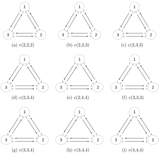
Consider a microarray experiment for 3 treatments and 6 arrays. If we assume that each treatment can have 2 or 3 or 4 independent biological replicates, then there are 9 different scenarios in total. By using the simulated annealing algo-rithm we have developed in the last section, we are able to find the (possibly near) L-optimal design for each of the scenarios. The results are represented in Figure
1 2 3 1 1 2 2 1 1 2 2 2 1 1 2 (a) c(2,2,2) 1 2 3 2 1 1 2 3 1 1 2 1 2 2 1 (b) c(2,2,3) 1 2 3 1 1 3 2 2 2 1 3 1 1 2 3 (c) c(2,3,3) 1 2 3 3 2 2 1 1 1 2 3 2 1 4 2 (d) c(2,3,4) 1 2 3 2 1 1 3 2 3 1 4 2 4 1 2 (e) c(2,4,4) 1 2 3 3 3 2 2 1 1 2 2 1 1 3 3 (f) c(3,3,3) 1 2 3 3 2 1 3 3 3 2 1 4 1 2 3 (g) c(3,3,4) 1 2 3 4 2 2 1 3 3 1 2 1 2 3 4 (h) c(3,4,4) 1 2 3 4 1 1 2 4 3 3 1 3 4 2 2 (i) c(4,4,4)
Figure 2.4: The L-optimal designs of microarray experiment for 3 treatments
and 6 arrays with respect to different combinations of numbers of independent biological replicates for each treatment. In the caption of subfigure, the notation c(x, y, z) is used to indicate that treatment 1, 2 and 3 has x, y, z independent biological
replicates respectively.
2.4. From the layouts, we see that each treatment uses as many biological repli-cates as possible: for treatments with enough biological replirepli-cates available (e.g. the treatments with 4 biological replicates), an independent biological replicate is used for each array it is involved with; for treatments with a limited number of biological replicates (i.e. less than the number of arrays on which they hybridize, like the treatments with only 2 biological replicates), the optimal design has to use technical replicates, i.e. repeats of certain biological replicates.
1 2 3 4 0.2 0.3 0.4 0.5 0.6 0.7 rho 1/L−optimality score c(2,2,2) c(2,2,3) c(2,3,3) c(2,3,4) c(2,4,4) c(3,3,3